Unitarity and Information in Quantum Gravity: A Simple Example

1. Introduction

The mathematical models that so far define our successful physical theories are all reversible in the sense that they can predict the future value of the variables they use from their initial values, while conversely the past can be uniquely reconstructed from the values of these variables in the future. The memory of the initial conditions is not lost in the dynamics and their information content remains. This is true for classical mechanics and field theory and it is also true for quantum mechanics and quantum field theory as long as we do not invoke the postulate of the collapse of the wave function (i.e., as long as we do not intervene from the outside via a measurement¹). In the quantum mechanical setting, this property boils down to the fact that evolution to the future is given by a unitary operator which can always be undone via its adjoint transformation.

This property of our fundamental models has always troubled naive intuition when faced with situations that appear to be irreversible. For example, what would happen to these words if the computer collapsed at this very moment? What if, after being printed, this paper is burned? Common sense would answer that the information in these pages (if of any relevance) would be lost. However, the physicist, trained to firmly believe in the statement of the previous paragraph, would say that the information in these words is not lost but simply hidden (to the point of becoming unrecoverable) in the humongous number of microscopic variables that would describe the whole system. In the case of burning the paper, these words remain “written” (it would be claimed) in the multiple correlations between the degrees of freedom of the molecules in the gas of the combustion diffusing in the atmosphere while transferring the information to even larger and yet pristine portions of the very large phase space of an unbounded universe. In the case where the computer collapses, a similar story can be told involving the dissipation of the bits into the environment. Of course the physicist cannot prove this; however, it is a consistent story in view of the strongly cherished principle of unitarity.

Such effective irreversibility is clearly captured in the second law of thermodynamics stating that (for suitable situations involving a large number of degrees of freedom) entropy can only increase. At the classical level this clashes at first sight with Liouville's theorem stating that the phase space volume of the support of a probability distribution is preserved by dynamical evolution. However, nothing restricts the shape of this volume to evolve into highly intricate forms that a macroscopic observer might be unable to resolve. More precisely, suitable initial conditions that the observer agent regards as special (for instance the macroscopic configurations of ink particles defining words in this paper before the fire reached them) come with an uncertainty in accordance to the observers limited measurement capabilities. This is idealized by a distribution in phase space occupying an initial phase space volume of a regular shape (this ensemble of points represents the system in what follows). Now as time goes by the apparent phase space volume (not the real volume which remains constant) would seem to grow to the agent just because of its intrinsic inability to separate the points in phase space that the systems occupies from the close neighboring ones where the system is not. The arrow of time (characterizing large systems) is only emergent macroscopically due to the special initial conditions, and the intrinsic coarse graining introduced by a macroscopic observer with its limitations. We will argue that the general lines of this story remain the same when black hole evaporation is considered.

General relativity combined with quantum field theory, in a regime where both are expected to be good approximations, imply that large isolated black holes behave like thermodynamical systems in equilibrium. They are objects close to equilibrium at the Hawking temperature that lose energy extremely slowly via Hawking radiation. When perturbed they come back to equilibrium to a new state and the process satisfies the first law of thermodynamics with an entropy equal to 1/4 of the area A of the black hole horizon in Planck units. Under such perturbation (which in particular can also be associated with their slow evaporation), the total entropy of the universe can only increase namely

$\begin{array}{ll}\delta S=\delta S_{\text{matter}}+\frac{\delta A}{4}\ge 0,& (1)\end{array}$

where δS_matter represents the entropy of whatever is outside the black hole (including, for instance, the emitted radiation).

This quasi equilibrium phase—which is extremely long lasting for macroscopic black holes but, at the same time, is only an intermediate situation before complete evaporation—is predicted by general relativity as the result of gravitational collapse taking place for suitable initial conditions. Indeed in order to make a black hole (BH), the past must be special (low entropy) too. Thus, the irreversibility captured by (1) can once more be associated with the same ingredients present in our previous example: the special nature of the initial conditions (low curvature and low densities in the past), high curvature, and huge new phase space regions available in the future; more precisely, in the Planckian regime that the singularity theorems of general relativity predict to develop inside the black hole horizon (the would-be-singularity from now on).

Such a perspective resonates with the one emphasized by Penrose (see for instance Penrose, 2005), among others: in full generality (now including gravity) the arrow of time comes from the fact that the universe is special in the past with a spacetime that was well-approximated by a homogeneous geometry and matter distribution (gas and dust) with tiny perturbations that would eventually grow and form galaxies and stars that one day can collapse to form black holes². Before the formation of a black hole, the story of our system exploring larger and larger portions of the available phase space is the usual standard involving molecules, atoms, and fundamental particles. The perspective we put forward here is that the story continues to be the same when black holes form and a new huge portion of phase space is opened by the physics of gravitational collapse. This new channel for entropy growth is opened by the appearance of the internal would-be-singularity of the classical description beyond the event horizon. The gravitational collapse ignites interactions with the Planckian regime inside the black hole horizon (see footnote 3), like the lighter setting the paper on fire and thus degrading the ink in the words when burning the paper in our previous discussion. The singularity predicted by general relativity brings the system in contact with the quantum gravity scale, and (as in the burning paper) this provides the key for resolving the puzzle of information in black hole evaporation.

This perspective, first advocated in Perez (2015, 2017), can be described with the help of Figure 1 (which applies to the general black hole formation and evaporation background scenario of reference; Ashtekar and Bojowald, 2005). The first assumption in the diagram is that there is evolution across the would-be-singularity (predicted by the classical dynamics) inside the black hole. This assumption is intrinsic in the representation in the figure; however, the scenario still makes sense if instead a baby universe is formed, i.e., if the would-be-singularity remains causally disconnected from the outside after evaporation. In that case, the correlations established with the baby universe remain hidden forever to outside observers. The virtue of the present scenario in such a case would be to give an identity to the degrees of freedom involved. The idea that the spacetime representation of the situation resembles the one in Figure 1 comes from the various results in symmetry-reduced models for both cosmology (Bojowald, 2001; Ashtekar et al., 2006) as well as for black holes (Modesto, 2004, 2006; Bojowald, 2005; Bojowald et al., 2005; Gambini and Pullin, 2013; Corichi and Singh, 2016; Ashtekar et al., 2018), and was first pictured in Ashtekar and Bojowald (2005). In such a context, a “scattering theory” representation (where an in-state evolves into an out-state) is possible even though the result (as we will argue) cannot be translated into the language of effective quantum field theory.

FIGURE 1

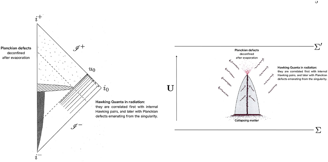
Figure 1. (Left) Penrose diagram illustrating (effectively) the natural scenario, suggested by the fundamental features of LQG, for the resolution of the information puzzle in black hole evaporation (Perez, 2015). The shaded region represents the would-be-singularity where high fluctuations in geometry and fields are present and where the low-energy degrees of freedom of the Hawking pairs are forced to interact with the fundamental Planckian degrees of freedom. (Right) Same situation as a scattering process from an initial to a final Cauchy hypersurface. This figure contains basically the same information as the Penrose diagram. Its additional merit, if any, is the more intuitive representation of the shrinking black hole as well as the time scales involved (collapse time is very short with respect to the evaporation time). Both these features are absent in the conformal representation on the left. There are limitations to this kind of spacetime representation of a process that is fundamentally quantum and hence only understandable in terms of superpositions of different spacetime geometries.

But what do we mean by a black hole in this evaporating context? In the asymptotically flat idealization, the black hole region is defined in classical general relativity as the portion of the spacetime ${M}$ that is not part of the past of ${I}$⁺. Such a definition needs to be modified in quantum gravity. In order to do that, we introduce the notion of the semiclassical past $J_C^{-}({{I}}^{+})$ of ${I}$⁺ as the collection of events in the spacetime that can be connected to ${I}$⁺ by causal curves along which the Kretschmann scalar $K\equiv R_{abcd}{R}^{abcd}\le \text{C}{\ell }_p^{-4}$ for some constant C of order unity. The black hole region can then be defined as

$\begin{array}{ll}B\equiv {M}-J_C^{-}({{I}}^{+}).& (2)\end{array}$

Its dependence on the constant C is not an important limitation in the discussion about information. Different C would lead to BH regions that coincide with Planckian corrections.

The most clear physical picture emerges from the analysis of the Penrose diagram on the left panel of Figure 1, from the point of view of observers at future null infinity ${I}$⁺. These observers are assumed to be at the center of the mass Bondi frame of the BH formed via gravitational collapse. We also assume that the Bondi mass of the BH is initially M ≫ m_p at some delayed time u on ${I}$⁺ representing the time where the BH has achieved its quasi-equilibrium state and starts evaporating slowly via Hawking radiation, i.e., the BH is initially macroscopic. Under such conditions the evaporation is very slow and we can trust the semiclassical description that suggests that the Bondi mass M(u) will slowly decrease with u from this initial value M until time u = u₀ (see figure) with M(u₀) ⪆ m_p in a time of the order of M³ in Planck units. From this time on, the details depend on a full quantum gravity calculation because the curvature around the BH horizon has become Planckian. Nevertheless, independently of such details we can safely say that the spacetime and the matter degrees of freedom encoded on ${I}$⁺ for u > u₀ must be in a superposition of states, all of which are very close to flat spacetime, as far as their geometry is concerned, with matter excitations very close to the vacuum because there is only at best an energy of the order of E_late ≈ m_p to substantiate both. In addition these excitations must be correlated with the early Hawking radiation with energy E_early ≈ M − m_p if unitarity is to hold. The late degrees of freedom are often referred to as purifying degrees of freedom.

One possibility is to assume that such purifying degrees of freedom are particle excitations coming from what is left of the BH (a remnant). Now, due to the fact that these particles must be extremely low-energy particles as only a total energy of E_late ≈ m_p is available for purification, a simple estimate of the time (denoted as τ_p) that the process would have to last if this is the main channel for purification yields ${\tau }_p\approx {(M/m_p)}^4$. This is the scenario of an extremely long lasting point-particle-like remnant with a huge internal degeneracy which is claimed to be problematic from the point of view of effective quantum field theory (Banks et al., 1993).

Instead we propose a different alternative: if smooth spacetime and matter fields are emergent notions from underlying discrete microscopic physics, then the coarse low-energy notion of classical geometry with smooth fields living on it would correspond in the fundamental Hilbert space to a very large set with (possibly) an infinite number of microscopic states. For instance the Minkowski vacuum unicity in standard quantum field theory would fail in the sense that the requirement that states look flat for (coarse-grained) low-energy observers—which are those for which an effective quantum field theory description in terms of smooth fields living on a smooth geometry is a suitable approximation—would still admit a highly degenerate ensemble of microscopic states (all states with total mass indistinguishable from zero by these macroscopic observers). Now, such low-energy modes cannot be identified with effective field theoretical excitations as the infrared excitations of fields mentioned in the previous paragraph (say low-energy photons). Like the molecular structure that escapes the smooth characterization of the Navier-Stokes effective theory of fluids, the degrees of freedom of interest here correspond to defects in the Planckian fabric of quantum gravity bound to be missed by coarse low-energy agents and their effective field theory mathematical models based on smoothness.

Why should information be hidden in the UV but not in the IR modes as in the remnant scenario mentioned above? It is often believed that because the volume inside the black hole actually becomes very large (according to suitable definitions; Christodoulou and De Lorenzo, 2016) then modes that are correlated with the Hawking radiation are redshifted and become highly IR inside. Although this is true for spherically symmetric Hawking quanta in the spherically symmetric Schwarzshild background—where such modes are indeed infinitely redshifted as detected by regular observers when they approach the singularity at r = 0—this conclusion fails when one considers no-spherical modes no matter how small the deviation from spherical symmetry is³. Therefore, generically all modes become UV close to the singularity [this is the central weakness of the bag-of-gold scenarios and the perspective proposed in Ashtekar (2020)].

We can draw a formal analogy with the Unruh effect as follows. The Unruh effect arises from the structure of the vacuum state |0〉 of a quantum field on the Minkowski spacetime when written in terms of the modes corresponding to Rindler accelerated observers with their intrinsic positive frequency notion. The vacuum takes the form

$\begin{array}{ll}|0\rangle ={\displaystyle \prod _k\left({\displaystyle \sum _n\exp }\left(-n\frac{\pi {\omega }_k}{a}\right)|n,k_R\rangle \otimes {|n,k\rangle }_L\right)},& (4)\end{array}$

where |n, k〉_L and |n, k〉_R define the particle modes—as viewed by an accelerated observer with uniform acceleration a—on the left and the right of the Rindler wedge (Wald, 1995). Here we see from the form of the previous expansion that even when we are dealing with a pure state (if we define the density matrix |0〉〈0|), the reduced density obtained by tracing over one of the two wedges would produce a thermal state with T = a/(2π). The statement in the perspective we propose on the purification of information in BH evaporation can be schematically represented (the following is certainly not a precise equation) by

$\begin{array}{l}U\underset{\text{quantum geometry}}{\underbrace{|flat,0\rangle }}\otimes \stackrel{\text{matter fields}}{\overbrace{|\varphi \rangle }}\\ ={\displaystyle \prod _k\left({\displaystyle \sum _n\exp }\left(-\frac{\beta }{2}n{\omega }_k\right)|flat,n\rangle \otimes |n,k\rangle \right)},& (5)\end{array}$

where an initial state of a flat quantum geometry |flat, 0〉 tensor product with a state representing initially diluted matter fields |ϕ〉 evolves unitarily via U into the formation of a BH and the subsequent evaporation (Figure 1) which after complete evaporation is written as a superposition of flat quantum geometry states |flat, n〉—which are all indistinguishable from |flat, 0〉 to low-energy agents and differ among them by quantum numbers n corresponding to quantities that are only measurable if one probes the state down to its Planckian structure—tensor product with normal n-particle excitations of matter fields representing Hawking radiation. As mentioned above, the previous equation is only a schematic. Its main inappropriateness is the fact that the reduced density matrix obtained by tracing over the quantum geometry hidden degrees of freedom would give a thermal state at a fixed temperature T. This is at odds with the expectation that the Hawking radiation should contain a superposition of the thermal radiation emitted at different Hawking temperatures during the long history of the evaporation of the BH. But the point that this equation and the discussion of the previous paragraph should make clear is that the purification mechanism proposed here has nothing to do with the point-like remnant scenario with all its problems associated with a long lasting particle-like remnant. In the present scenario, to the future of the would-be-singularity in Figure 1, we simply have a quantum superposition of different quantum geometry states that all look flat to low-energy observers. There are no localized remnants hiding in the huge internal degeneracy; there is only a large superposition of states that are inequivalent in the fundamental quantum gravity Hilbert space but seem identical when tested with low-energy probes. Such degrees of freedom cannot be captured by any effective description in terms of smooth fields (EQFT) for the simple reason that they are discrete in their fundamental nature.

Notice that the degrees of freedom, where information would be coded after BH evaporation, do not satisfy the usual Einstein-Planck relationship E = ℏω or equivalently p = h/λ (for some “wavelength” λ or “frequency” ω), and this might deceive intuition⁴. These are Planckian defects yet they do not carry Planckian energy. The point is that such a relationship only applies under suitable conditions which happen to be met in many cases but do not need to always be valid. One case is the one of degrees of freedom that can be thought of as waves moving on a preexistent spacetime. This is the case for particle excitations in the Fock space of quantum field theory or effective quantum field theories (both of which are defined in terms of a preexistent spacetime geometry). There is no clear meaning to the above intuitions in the full quantum gravity realm where the present discussion is framed. Even when such relations (linked to the usual uncertainty principle of quantum mechanics) should hold in a suitable sense—if the structure suggested by canonical quantization survives in quantum gravity as it should to a certain degree—they would apply to phase space variables encoding to the true degrees of freedom of gravity that we expect (from general covariance) to be completely independent of a preexistent background geometry. We will see that such degrees of freedom with such a peculiar nature actually arise naturally in the toy model of quantum gravity that we analyze in this article.

It is presently hard to prove that such a scenario is viable in a quantum theory of gravity simply because there is no such theoretical framework developed enough for tackling BH formation and evaporation in detail. However, the application of loop quantum gravity to quantum cosmology leads to a model with similar features, where evolution across the classical singularity is well defined (Bojowald, 2001). The results have been reported in Amadei and Perez (2019). In this article we present the main features of this model in more detail and show that the conclusions of Amadei and Perez (2019), some of which are drawn from some simplified models of matter coupling, are generic and remain true in more physically realistic models.

The results can be described briefly by making reference to Figure 2 which should be compared with the right panel in Figure 1. We will show that the evolution in loop quantum cosmology from a universe in an initially contracting state in the past of the would-be-singularity to an expanding universe in its future is perfectly unitary in its fundamental description. Nevertheless, states in the Hilbert space of loop quantum cosmology contain quantum degrees of freedom which are hidden to low-energy coarse-grained observers. If these degrees of freedom are traced out in the initial density matrix then we will see that pure states (in the sense of the reduced density matrix) generically evolve into mixed states across the would-be-singularity. Information is lost in correlations with degrees of freedom that are Planckian and thus inaccessible to macroscopic observers. These correlations are established in an inevitable way during the strong curvature phase of evolution across the big bang (just as expected in the BH scenario described above). As energy is conserved (energy is a delicate notion in cosmology but happens to be well-defined in our model as we will see), the defects that purify the final state do not enter into the energy balance which realizes another crucial necessary ingredient of the general scenario (decoherence happens with negligible dissipation; Unruh, 2012).

FIGURE 2

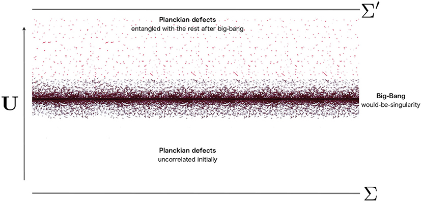
Figure 2. Diagram (effectively) illustrating the natural scenario, suggested by the fundamental features of LQG, for the resolution of the information puzzle in black hole evaporation (Perez, 2015). As in Figure 1, one should keep in mind the limitations of this kind of spacetime representation of a process that is fundamentally quantum and hence only understandable in terms of superpositions of different spacetime geometries.

The paper is organized as follows. In the first part (section 2), we show that the scenario we have described in general terms so far is realized in unimodular quantum cosmology following the standard quantization prescription of loop quantum cosmology. Aside from a different choice of time variable, the model of this section is exactly equivalent to other models studied in the standard literature (Ashtekar and Singh, 2011). In the second part of the paper, we observe that there is natural extension of loop quantum cosmology based on the regularization ambiguity associated with the quantization of the Hamiltonian. This extension provides another interesting realization of our mechanism. Although this second option is not necessary to illustrate our point (already realized in the standard theory in the first part), it gives a different identity to the defects which could lead to independent and thus useful insights. We have included a series of appendices where some calculations are shown. Appendix D is especially important because some of the over-simplified model (analytic) calculations in the body of the paper are completed (numerically) using a more physically realistic case of the coupling of gravity with a massless scalar field.

2. Unimodular Gravity: Four-Volume as Time

In this section we introduce the basic structure of quantum unimodular gravity in the framework of quantum cosmology. This theory will provide us with a toy model to study the unitary evolution of the state of the universe across the big-bang singularity. We will see that the Hilbert space of loop quantum cosmology contains the type of microscopic degrees of freedom evoked in the general discussion of the introduction. This is a minimalistic model where our scenario can be explicitly realized.

Unimodular gravity as a concept is nearly as old as general relativity itself, it was introduced by Einstein in 1919 (Einstein, 1919) as an attempt to describe nuclear structure geometrically. In his work, Einstein also identified an appealing feature of the theory, which is the fact that the cosmological constant arises as a dynamical constant of motion that needs to be added to the initial values of the theory. In unimodular gravity, the cosmological constant is a constant of integration and not a universal or fundamental constant of nature. Interest in the theory was regained in the late 80's with the observation of Weinberg (1989) that, for the above reason, semiclassical unimodular gravity provides a trivial resolution of the cosmological constant problem as vacuum energy simply does not gravitate. Unimodular gravity is the natural low-energy description that emerges from the formal thermodynamical ideas of Jacobson (1995), and represents the expected low energy regime of the causal set approach (Bombelli et al., 1987).

Another property of unimodular gravity (specially important for us here) is that it completely resolves the problem of time (Unruh, 1989) in the cosmological FLRW context. More precisely, the theory comes with a preferred time evolution and a preferred Hamiltonian (the energy of the universe is well defined and directly linked with the value of the cosmological constant). The quantum theory is described by a Schrodinger-like equation where states of the universe are evolved by a unitary evolution operator. Therefore, unlike the general situation in quantum gravity, the notion of unitarity is unambiguously defined in unimodular quantum cosmology. This is the main reason why unimodular gravity provides the perfect framework for the discussion of the central point of this work.

Here we specialize in homogeneous and isotropic cosmologies that are spatially flat (k = 0), i.e., the spatial manifold Σ is topologically ℝ³. What follows is the standard construction. For a detailed account of the Hamiltonian analysis in the cosmological framework (see Chiou and Geiller, 2010). The FLRW metric is

$\begin{array}{ll}d{s}^2=-N{(t)}^{2}d{t}^2+a{(t)}^2{\displaystyle \underset{q_{ab}}{{\displaystyle \underbrace{(d{x}^2+d{y}^2+d{z}^2)}}}},& (6)\end{array}$

where q_ab denotes the fiducial spacial metric. Since Σ is non-compact, some integrals are infrared divergent and are regularized by restricting them to a fixed fiducial cell ${V}$ of fiducial volume V₀ with respect to the fiducial spacial metric

$\begin{array}{ll}{q}_{ab}=e_a^i{e}_b^j{\delta }_{ij},& (7)\end{array}$

where $e_a^i$ denotes a fiducial triad and the physical metric is given by $q_{ab}=a^2(t)q_{ab}$. The action of unimodular gravity in the FLRW mini superspace setup is given by

$\begin{array}{llll}S[a,ȧ,\lambda ]& =& \frac{3}{8\pi G}{\displaystyle {\int }_{ℝ}}\left(\frac{V_{0}a{ȧ}^2}{N}+\lambda V_0(N{a}^3-1)\right)dt,& (8)\end{array}$

where λ is a Lagrange multiplier imposing the unimodular constraint N = a⁻³ (i.e., $\sqrt{\left|g\right|}=1$), and the first term is the Einstein-Hilbert action restricted to the FLRW geometries⁵. In order to use loop quantum cosmology techniques (for a discussion of the quantization in the full loop quantum gravity context; see Smolin, 2009, 2011), one introduces the new canonical variables c and p via the basic Ashtekar-Barbero connection variables $A_a^i$ and $E_i^a$, namely

$\begin{array}{ll}{E}_i^a=p\left(e_i^a{V}_0^{-2/3}\right),A_a^i=c\left({\omega }_a^i{V}_0^{-1/3}\right),& (9)\end{array}$

where ${\omega }_a^i$ is a fiducial reference connection. These variables are related to those in (8) via the equations

$\begin{array}{ll}\left|p\right|=V_0^{2/3}{a}^2,c=V_0^{1/3}\frac{\gamma ȧ}{N}.& (10)\end{array}$

The action becomes

$\begin{array}{ll}S[c,p,\lambda ]=\frac{3}{8\pi G}{\displaystyle {\int }_{ℝ}}{\gamma }^{-1}cṗ-N{\gamma }^{-2}\sqrt{|p|}{c}^2+\lambda (N|p{|}^{\frac{3}{2}}-V_0)dt,& (11)\end{array}$

and c and p are canonically conjugated in the sense that

$\begin{array}{ll}\{c,p\}=\frac{8\pi G\gamma }{3}.& (12)\end{array}$

The unimodular condition N = a⁻³ fixes the lapse to $N=V_0/|p{|}^{3/2}$ and the unimodular Hamiltonian becomes

$\begin{array}{ll}H=\frac{3V_0}{8\pi G}\frac{c^2}{{\gamma }^2\left|p\right|}.& (13)\end{array}$

The proportionality of the Hamiltonian with V₀, and the fact that the four-volume bounded by V₀ at two different times is given by $v^{(4)}=V_0\Delta t$, implies that time evolution can be parameterized in terms of the four-volume elapsed from some reference initial slice. The associated Hamiltonian [conjugated to v⁽⁴⁾/(8πG)] is

$\begin{array}{ll}\Lambda =\frac{3c^2}{{\gamma }^2|p|},& (14)\end{array}$

and corresponds to the cosmological constant.

2.1. Quantization

The loop quantum cosmology quantization uses a non standard representation of the canonical variables where the variable c does not exist as a quantum operator, and the definition of the Hamiltonian requires a special regularization procedure known as the $\stackrel{-}{\mu }$-scheme (Ashtekar and Singh, 2011). The quantization prescription is greatly simplified by the introduction of new canonically conjugated dynamical variables b and ν defined as (Ashtekar et al., 2008)

$\begin{array}{ll}b\equiv \frac{c}{|p{|}^{\frac{1}{2}}}\nu \equiv \text{sign}(p)\frac{|p{|}^{\frac{3}{2}}}{2\gamma \pi {\ell }_p^2},& (15)\end{array}$

with Poisson brackets⁶

$\begin{array}{ll}\{b,\nu \}=2{\hslash }^{-1}.& (16)\end{array}$

The variable ν corresponds to the physical volume of the fiducial cell divided by ${\ell }_p^2$; it has units of distance. The variable b is simply its conjugate momentum. In terms of these variables the gravitational (unimodular) Hamiltonian (13) integrated in a fiducial cell V becomes

$\begin{array}{ll}H=\frac{3V_0}{8\pi G{\gamma }^2}{b}^2.& (17)\end{array}$

Note the extreme simplicity of the previous expression: the unimodular Hamiltonian is just the analog of that of a free particle in one dimension with a mass parameter of $m=4\pi {\gamma }^2/(3V_0)$ and momentum b. In the absence of matter, the Hamiltonian can be quantized in the Wheeler-DeWitt representation where the evolution in unimodular time is unitary and there is no singularity (the classical solutions correspond to De-Sitter geometries with arbitrary but positive cosmological constants). The singularity in the classical theory becomes real when matter is introduced.

In the loop quantum cosmology polymer representation, just as for c, there is no operator corresponding to b but only the operators corresponding to finite ν translations (Ashtekar et al., 2006); from here on referred to as shift operators

$\begin{array}{ll}exp(i2kb)⊳\Psi (\nu )=\Psi (\nu -4k).& (18)\end{array}$

For $k=q\sqrt{\Delta }{\ell }_p$ and q ∈ ℕ, states that diagonalize the previous shift operators, denoted $|b_0;{\Gamma }_{\Delta }^{ϵ}\rangle$, are labeled by a real value b₀ and by a graph ${\Gamma }_{\Delta }^{ϵ}$. The graph is a 1D lattice of points in the real line of the form $\nu =4n\sqrt{\Delta }{\ell }_p+ϵ$ with $ϵ\in [0,4\sqrt{\Delta }{\ell }_p)$ and n ∈ ℕ. The corresponding wave function is given by ${\text{Ψ}}_{b_0}(\nu )\equiv \langle \nu |b_0;{\Gamma }_{\Delta }^{ϵ}\rangle =exp(-i\frac{b_0\nu }{2}){\delta }_{{\Gamma }_{\Delta }^{ϵ}}$, where the symbol ${\delta }_{{\Gamma }_{\Delta }^{ϵ}}$ means that the wavefunction vanishes when $\nu \notin {\Gamma }_{\Delta }^{ϵ}$. It follows from (18) that

$\begin{array}{ll}\exp (i2kb)⊳|b_0;{\Gamma }_{\Delta }^{ϵ}\rangle =\exp (i2k{b}_0)|b_0;{\Gamma }_{\Delta }^{ϵ}\rangle .& (19)\end{array}$

The states $|b;{\Gamma }_{\Delta }^{ϵ}\rangle$ are eigenstates of the shift operators that preserve the lattice ${\Gamma }_{\Delta }^{ϵ}$. Notice that the eigenvalues are independent of the parameter ϵ, i.e., they are infinitely degenerate and span a non separable subspace of the quantum cosmology Hilbert space ${H}$_lqc.

A scale $\stackrel{-}{\mu }$ is needed in order to define a regularization of (17) representing the Hamiltonian in ${H}$_lqc. The reason is that there are no operators associated with b but only approximants constructed via the shift operators (18). The so-called $\stackrel{-}{\mu }$-scheme (Ashtekar and Singh, 2011) introduces a dynamical length scale $\stackrel{-}{\mu }$ defined as

$\begin{array}{ll}{\overline{\mu }}^2=\frac{{\ell }_p^2\Delta }{\left|p\right|},& (20)\end{array}$

where Δ represents the so-called “area-gap” which plays the role of a UV regulator. It is normally associated with the smallest non-vanishing area quantum in the full theory of loop quantum gravity. For the moment (as in the standard treatment), this is just a fixed parameter⁷. When translated into the variables (15), $\overline{\mu }$ corresponds to considering approximants to b constructed out of shift operators (18) with fixed $k\equiv \sqrt{\Delta }{\ell }_p$. In terms of these, one obtains the following regularization of the Hamiltonian (17) which is a well-defined self-adjoint operator⁸ acting on ${H}$_lqc

$\begin{array}{ll}{H}_{\Delta }\equiv \frac{3V_0}{8\pi G{\gamma }^2}\frac{1}{\Delta {\ell }_p^2}{sin}^2\left({\Delta }^{\frac{1}{2}}{\ell }_{p}b\right),& (21)\end{array}$

which coincides with (17) leading to (zero) order in ${\ell }_p^2$. From (14), we obtain an operator associated to the (here dynamical) cosmological constant, namely

$\begin{array}{ll}{\Lambda }_{\Delta }\equiv \frac{3}{{\gamma }^2}\frac{{sin}^2\left({\Delta }^{\frac{1}{2}}{\ell }_{p}b\right)}{\Delta {\ell }_p^2}.& (22)\end{array}$

In the pure gravity case, the cosmological constant is positive definite and bounded from above by the maximum value ${\text{λ}}_{\text{max}}=1/({\gamma }^2{\ell }_p^2\Delta )$. Negative cosmological constant solutions are possible when matter is added (see Appendix B). The states (19) with $k=k_{\Delta }\equiv \sqrt{\Delta }{\ell }_p$ diagonalize the Hamiltonian, i.e.,

$\begin{array}{ll}{H}_{\Delta }⊳|b_0;{\Gamma }_{\Delta }^{ϵ}\rangle =E_{\Delta }(b_0)|b_0;{\Gamma }_{\Delta }^{ϵ}\rangle ,& (23)\end{array}$

with energy eigenvalues

$\begin{array}{ll}{E}_{\Delta }(b_0)=\frac{3V_0}{8\pi G{\gamma }^2}\frac{1}{\Delta {\ell }_p^2}{sin}^2\left({\Delta }^{\frac{1}{2}}{\ell }_p{b}_0\right).& (24)\end{array}$

States $|b_0;{\Gamma }_{\Delta }^{ϵ}\rangle$ are also eigenstates of the cosmological constant with eigenvalue λ_Δ(b₀) = (8πG)E_Δ(b₀)/V₀. Notice that the energy eigenvalues do not depend on $ϵ\in [0,4\sqrt{\Delta }{\ell }_p)$. Thus, the energy levels are infinitely degenerate with energy eigenspaces that are non-separable. This is not something peculiar of our model but a general property of the non-standard representation of the canonical commutation relations used in loop quantum cosmology.

2.2. On the Interpretation of the ϵ Sectors

It is customary in the loop quantum cosmology literature to restrict to a fixed value of ϵ in concrete cosmological models, as the dynamical evolution does not mix different ϵ sectors. The terminology “superselected sectors” is used in a loose way in discussions. However, these sectors are not superselected in the strict sense of the term because they are not preserved by the action of all the possible observables in the model, i.e., there are non trivial Dirac observables mapping states from one sector to another. The explicit construction of such observables might be very involved in general (as is the usual case with Dirac observables); nevertheless, it is possible to exhibit them directly at least in one simple situation: the pure gravity case. In that case, the shift operator (18) with shift parameter δ commutes with the pure gravity Hamiltonian (the Hamiltonian constraint if we were using standard loop quantum cosmology) and maps the ϵ sector to the ϵ − 4δ sector. The analogous Dirac observables in a generic matter model can be formally described with techniques of the type used for the definition of evolving constants of motion (Rovelli, 1991). No matter how complicated this might be in practice, the point is well-illustrated by our explicit example in the matter free case⁹.

Thus, different ϵ sectors are not superselected and therefore the infinite degeneracy of the energy eigenvalues of the Hamiltonian (which again we exhibit explicitly in the previous discussion only in the vacuum case) must be taken at face value. How can we understand this large degeneracy from the fact that there would be only a two-fold degeneracy (associated with a contracting or expanding universe) if we had quantized the model using the standard Schrodinger representation or, in other words, the standard Wheeler-DeWitt quantization? The answer is to be found, we claim, in the notion of coarse graining: low-energy observers only distinguish a two-fold degeneracy for energy (or cosmological constant) eigenvalues: one the universe has a given cosmological constant, and two it is expanding or contracting. These are the quantum numbers in the Wheeler-DeWitt quantization which play a role in our context of the low-energy effective quantum field theory formulation. Such coarse observers are declared to be insensitive to the huge additional degeneracy of energy eigenstates encoded in the quantum number ϵ. All these infinitely many states in the quantum cosmology representation must be considered as equivalent to the two-fold degeneracy mentioned above.

In what follows, and for concreteness, we will consider combinations of states with two different values for ϵ only, i.e., on two different lattices. The idea of the previous paragraph will naturally produce a notion of coarse-graining entropy associated with the intrinsic statistical uncertainty due to the inability for a low-energy agent to distinguish these microscopically orthogonal states. Arbitrary superposition with N different ϵ sectors would lead to similar results [the entropy capacity growing with the usual log(N)]. The N = 2 case treated here renders some explicit calculations straightforward.

2.3. Matter Couplings and a Model Capturing Its Essential Features

Here we discuss two simple matter models in order to isolate the generic features of the influence of matter. At the end of the section, we will define a simple and trivially solvable model capturing these features.

Perhaps the simplest matter model that would serve our purposes is minimal and isotropic coupling to a Dirac fermion defined in de Berredo-Peixoto et al. (2012). After symmetry reduction, the action for matter is

$\begin{array}{ll}{S}_{\text{F}}(\eta ,\overline{\eta })=V_0{\displaystyle {\int }_{ℝ}d}\tau \left[\frac{i}{2}a{(\tau )}^3\left(\overline{\eta }{\gamma }^0\dot{\eta }-\dot{\overline{\eta }}{\gamma }^0\eta \right)-mN(\tau )a{(\tau )}^3\overline{\eta }\eta \right],& (25)\end{array}$

from which we read the fermionic contribution to the Hamiltonian

$\begin{array}{l}{H}_{\text{F}}=mN(\tau )a^3(\tau )\overline{\eta }\eta =-mN(\tau )p_{\eta }{\gamma }_0\eta \\ =\frac{m}{a^3}{p}_{\eta }{\gamma }_0\eta ,& (26)\end{array}$

where (Π, Ψ) are the fermionic canonical variables $\Pi \equiv {(V_{0}a)}^{3/2}{\psi }^{†}$ and $\Psi \equiv {(V_{0}a)}^{3/2}\psi$ (Thiemann, 2001), and in the second line, we use the unimodular condition $N=V_0^{-1}{a}^{-3}$. In the quantum theory, the non trivial anti-commutator is {η, p_η} = 1 with the rest equal to zero. This is achieved by writing $\eta =\sum _s\left(a_s{u}^s{e}^{-imt}+b_s^{†}{v}^s{e}^{imt}\right)$ with non trivial anti-commutation relations for the creation and annihilation of operators $\{a_r,a_s^{†}\}={\delta }_{rs}=\{b_r,b_s^{†}\}$, with u^se^−imt and $v_s{e}^{imt}$ as a complete basis of solutions of the Dirac equation for positive and negative frequency, respectively (Peskin and Schroeder, 1995). In our model, we can have either the vacuum state, or one or two fermions which saturate the Pauli exclusion principle. If we assume normal ordering, the contribution to the unimodular energy is

$\begin{array}{ll}{H}_{\text{F}}=\frac{mn}{a^3}.& (27)\end{array}$

where n = 0, 1, 2 is the occupation number for the fermion. If instead of the condition $N=V_0^{-1}{a}^{-3}$, we had used N = 1 (where time is comoving time) then the energy contribution would have been just m for which we have a clear physical intuition: a single fermion homogeneously distributed in the universe contributes to the Hamiltonian with its total mass. The factor 1/a³ in the previous expression comes from the unimodular condition.

In the case of Wheeler-DeWitt quantization, the contribution of the fermion becomes singular at the big bang a = 0. In loop quantum cosmology, such a quantity remains bounded above due to loop quantum gravity discreteness. Indeed, using the inverse volume quantization given in reference (Ashtekar and Singh, 2011), one has

$\begin{array}{ll}{\widehat{H}}_{\text{F}}⊳|\psi \rangle =-m{\displaystyle \sum _{\nu }}|\nu \rangle h_{\text{F}}(\nu ;\sqrt{\Delta }{\ell }_p)\Psi (\nu ,\eta ),& (28)\end{array}$

where

$\begin{array}{ll}{h}_{\text{F}}(\nu ;\lambda )\equiv \frac{1}{4{\lambda }^2}{\left(|\nu +2\lambda {|}^{\frac{1}{2}}-|\nu -2\lambda {|}^{\frac{1}{2}}\right)}^2.& (29)\end{array}$

We notice that $h_{\text{F}}(\nu ;\sqrt{\Delta }{\ell }_p)<1$ and decays like 1/ν for ν → ∞¹⁰. One could, in principle, add this term to the free Hamiltonian and solve the unimodular time-independent Schrodinger equation

$\begin{array}{ll}({\widehat{H}}_0+{\widehat{H}}_{\text{F}})⊳|\psi \rangle =E|\psi \rangle .& (30)\end{array}$

Solutions can be interpreted in the sense of scattering theory starting with free wave packets for large ν picked around a value of the cosmological constant (22) or energy (24).

The case of coupling with a scalar field is formally very similar, especially in the simplified case where we assume it to be massless. Following Ashtekar and Singh (2011), and using the unimodular condition N = a⁻³, we get

$\begin{array}{ll}{H}_{\varphi }=-\frac{p_{\varphi }^2}{8{\pi }^2{\gamma }^2{\ell }_p^4{\nu }^2}.& (31)\end{array}$

This leads to

$\begin{array}{ll}{\widehat{H}}_{\varphi }⊳|\psi \rangle =-m{\displaystyle \sum _{\nu }}|\nu \rangle h_{\varphi }(\nu ;\sqrt{\Delta }{\ell }_p)\Psi (\nu ,\varphi ),& (32)\end{array}$

where

$\begin{array}{ll}{h}_{\varphi }(\nu ;\lambda )\equiv \frac{p_{\varphi }^2}{16{\lambda }^4}{\left(|\nu +2\lambda {|}^{\frac{1}{2}}-|\nu -2\lambda {|}^{\frac{1}{2}}\right)}^4.& (33)\end{array}$

The momentum p_ϕ commutes with the Hamiltonian and thus it is a constant of motion. If we consider an eigenstate of p_ϕ then the problem reduces again to a scattering problem with a potential decaying like 1/ν² when we consider solving the time-independent Schrodinger equation

$\begin{array}{ll}({\widehat{H}}_0+{\widehat{H}}_{\varphi })⊳|\psi \rangle =E|\psi \rangle .& (34)\end{array}$

Therefore, both the fermion as well as the scalar field models (which are closer to a possibly realistic scenario) seem tractable with a slight generalization of the standard scattering theory to the discrete loop quantum cosmology setting. However, the main objective in this section is to illustrate an idea in terms of a concrete and simple toy model. With this idea in mind, we will modify the structure suggested by the fermion coupling and the scalar field coupling and simply add an interaction term where the “long-distance interaction” term represented by the function F(ν; λ) is replaced by a short-range analog F(ν; λ) ∝ δ_{ν, 0}. The qualitative properties of the scattering will be the same and the model becomes sufficiently trivial for straightforward analytic computations. The results for the more realistic free scalar field model have been dealt with numerically and are presented in Appendix D.

For that we consider an interaction that begins at ν = 0:

$\begin{array}{ll}\widehat{H}={\widehat{H}}_0+\mu {\widehat{H}}_{\text{int}},& (35)\end{array}$

where μ is a dimensionless coupling, Ĥ₀ is given in (58), and Ĥ_int is

$\begin{array}{ll}{\widehat{H}}_{\text{int}}⊳|\psi \rangle \equiv {\displaystyle \sum _{\nu }\left({\ell }_p^{-4}\frac{V_0}{\sqrt{\Delta }}\right)}|\nu \rangle \frac{{\delta }_{\nu ,0}}{\sqrt{\Delta }}\Psi (0).& (36)\end{array}$

We have added by hand an interaction Hamiltonian that switches on only when the universe evolves through the would-be-singularity at the zero volume state. The key feature of the Ĥ_int is that—as its more realistic relatives, matter Hamiltonians (28) and (32)—it breaks translational invariance and thus, it leads to different dynamical evolution for different ϵ sectors.

2.4. Solutions as a Scattering Problem

The scattering problem is very similar to the standard one in one-dimensional quantum mechanics; however, one needs to take into account the existence of the peculiar degeneracy of energy eigenvalues contained in the ϵ sectors; see sections 2.1 and 2.2. We will consider, for simplicity, the superposition of only two states supported on two lattices respectively: the lattice ${\Gamma }_{\Delta }^{ϵ}$ with ϵ = 0 for the first one and the one with $ϵ=2\sqrt{\Delta }{\ell }_p$ for the second one. The degenerate eigenstates of the shift operators (19) with eigenvalues exp(i2kb) will be denoted as

$\begin{array}{ll}|b,1\rangle \equiv |b;{\Gamma }_{\Delta }^0\rangle , \text{and} |b,2\rangle \equiv |b;{\Gamma }_{\Delta }^{2\sqrt{\Delta }{\ell }_p}\rangle ,& (37)\end{array}$

respectively, while we will denote Γ¹ and Γ² as the corresponding underlying lattices. The immediate observation is that states supported on Γ² (superpositions of |b, 2〉) will propagate freely because they are supported on a lattice that does not contain the point ν = 0 where the interaction is non trivial. On the other hand, states supported on Γ¹ (superpositions of |b, 1〉) will be affected by the interaction at the big bang. Before and after the big bang, the universe's evolution of the second type of states is well described by the eigenstates of the Hamiltonian (58) described in section 2.1. Such asymmetry of the interaction on different ϵ sectors is not an artifact of the simplicity of the interaction Hamiltonian. This is just a consequence of the necessary breaking of the shift invariance for any realistic matter interaction as we argued in the previous section and we show explicitly in Appendix D (see Figure 3).

FIGURE 3

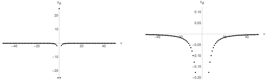
Figure 3. The function h_ϕ(ν; λ) evaluated on an ϵ sector containing ν = 0, for p_ϕ = 10 in natural units and λ = 1/2 is plotted using two different ranges. On the left, we see that the function is finite near ν = 0. On the right, we can see that it behaves like −ν⁻² for large values of ν. This function can be seen as the effective potential where an asymptotically free state of the universe (pure gravity with cosmological constant state or asymptotically de Sitter state) scatters. If the cosmological constant is negative there are bound states whose superposition can be used to define semiclassical universes oscillating in an endless series of big bangs and big crunches (see section B).

Therefore, the non trivial scattering problem concerns only states on the lattice ${\Gamma }^1=\{\nu =4n\sqrt{\Delta }{\ell }_p|n\in \mathbb{Z}\}$ that is preserved by the Hamiltonian and contains the point ν = 0. In order to solve the scattering problem, we consider an in-state of the form

$\begin{array}{ll}|{\psi }_k\rangle =|\nu \rangle \{\begin{array}{cc}{e}^{-i\frac{k}{2}\nu }+A(k)e^{i\frac{k}{2}\nu }& \text{(}\nu \ge 0\text{)}\\ B(k)e^{-i\frac{k}{2}\nu }& \text{(}\nu \le 0\text{)},\end{array}& (38)\end{array}$

where ν ∈ Γ¹, and A(k) and B(k) are coefficients depending on k. For suitable coefficients, such states are eigenstates of the full Hamiltonian (35). Arbitrary solutions (wave packets) can then be constructed in terms of appropriate superpositions of these “plane-wave” states.

We can compute the scattering coefficients A(k) and B(k) from the discrete (finite difference) time-independent Schrodinger equation

$\begin{array}{ll}\left({\widehat{H}}_0+{\widehat{H}}_{int}\right)⊳|\psi \rangle =E|\psi \rangle & (39)\end{array}$

which amounts to the following finite difference equation in the ν basis:

$\begin{array}{l}{\displaystyle \sum _v(-\frac{3V_0}{8\pi G{\gamma }^2}\frac{1}{2\Delta {\ell }_p^2}[\Psi (\nu -4\sqrt{\Delta }{\ell }_p)+\Psi (\nu +4\sqrt{\Delta }{\ell }_p)}\\ -2\Psi (\nu )]+\frac{V_0\mu }{\Delta {\ell }_p^4}{\delta }_{\nu ,0}\Psi (0)-E(k)\Psi (\nu ))|\nu \rangle =0.\end{array}$

The matching conditions on ν = 0 are given by:

$\begin{array}{l}1+A(k)=B(k)\\ -\frac{3}{16\pi G{\gamma }^2\Delta {\ell }_p^2}\left[\Psi (-4\sqrt{\Delta }{\ell }_p)+\Psi (4\sqrt{\Delta }{\ell }_p)-2\Psi (0)\right]\\ +\frac{\mu }{\Delta {\ell }_p^4}\Psi (0)=\frac{E(k)}{V_0}\Psi (0),\end{array}$

where the first equation comes from continuity at ν = 0, the second equation from the time-independent Schrodinger equation. The solution of the previous equations is

$\begin{array}{l}\begin{array}{c}A(k)=\frac{-i\Theta (k)}{1+i\Theta (k)}\end{array}\\ \begin{array}{c}B(k)=\frac{1}{1+i\Theta (k)}\end{array}& (40)\end{array}$

where

$\begin{array}{ll}\Theta (k)\equiv \frac{16\pi {\gamma }^2}{3}\frac{\mu }{sin(2k\sqrt{\Delta }{\ell }_p)}.& (41)\end{array}$

We consider an in-state of the form (valid for early times)

$\begin{array}{ll}|{\psi }_{in},t\rangle =\frac{\pi }{\sqrt{2\Delta }{\ell }_p}{\displaystyle \int db(\psi (b;b_0,{\nu }_0)|b,1\rangle +\psi (b;b_0,{\nu }_0)|b,2\rangle )e^{-i{E}_{\Delta }(b)t},}& (42)\end{array}$

where ψ(b; b₀, ν₀) is a wave function picked at a b = b₀ value and ν = ν₀. Notice that we are superimposing two wave packets supported on lattices Γ¹ and Γ², respectively. We can now write the pure in-density matrix

$\begin{array}{l}{\rho }_{\text{in}}(t)=\frac{{\pi }^2}{2\Delta {\ell }_p^2}{\displaystyle \int }dbd{b}^{\prime }{e}^{i[E_{\Delta }(b)-E_{\Delta }(b^{\prime })]t}\\ \times \left[|b^{\prime },1\rangle \psi (b^{\prime };b_0,{\nu }_0)+|b^{\prime },2\rangle \psi (b^{\prime };b_0,{\nu }_0)\right]& (43)\end{array}$

$\begin{array}{ll}\left[\langle b,1|\overline{\psi }(b;b_0,{\nu }_0)+\langle b,2|\overline{\psi }(b;b_0,{\nu }_0)\right]& (44)\end{array}$

which scatters into the out-density matrix

$\begin{array}{l}{\rho }_{\text{out}}(t)=\frac{{\pi }^2}{\Delta {\ell }_p^2}{\displaystyle \int d}bdb\prime e^{i[E_{\Delta }(b)-E_{\Delta }(b\prime )]t}\\ [\langle b,1|\overline{\psi }(-b;b_0,{\nu }_0)\overline{A}(-b)+\langle b,1|\overline{\psi }(b;b_0,{\nu }_0)\overline{B}(b)\\ +\langle b,2|\overline{\psi }(b;b_0,{\nu }_0)]\\ [|b^{\prime },1\rangle \psi (-b\prime )e^{-ib\prime \overline{\nu }}A(-b\prime )+|b^{\prime },1\rangle \psi (b\prime )e^{ib\prime \overline{\nu }}B(b\prime )\\ +|b^{\prime },2\rangle \psi (b\prime ;b_0,{\nu }_0)].\end{array}$

Let us assume that ψ(b) is highly picked at a b₀ so that we can substitute the integration variables b and b′ by b₀ and have a finite dimensional representation of the reduced density matrix after the scattering (this step is rather formal, it involves an approximation but it helps when visualizing the result). In the relevant 4 × 4 sector (with basis elements ordered as {|1, b₀〉, |1, −b₀〉, |2, b₀〉, |2, −b₀〉}), we get the matrix representation

$\begin{array}{l}{\rho }_{in}=\left(\begin{array}{cccc}\frac{1}{2}& 0& \frac{1}{2}& 0\\ 0& 0& 0& 0\\ \frac{1}{2}& 0& \frac{1}{2}& 0\\ 0& 0& 0& 0\end{array}\right)\to {\rho }_{out}\\ =\frac{1}{2}\left(\begin{array}{cccc}|B(b_0){|}^2& \overline{A}(-b_0)B(b_0)& B(b_0)& 0\\ A(-b_0)\overline{B(b_0)}& |A(-b_0){|}^2& A(-b_0)& 0\\ \overline{B(b_0)}& \overline{A(-b_0)}& 1& 0\\ 0& 0& 0& 0\end{array}\right).& (45)\end{array}$

2.5. Matter Coupling Produces a Coarse-Graining Entropy Jump at the Big Bang

A reduced density matrix encoding the notion of coarse graining associated with the low-energy equivalence of the ϵ sectors is defined by tracing over the discrete degrees of freedom labeling the component of the state in either the Γ₁ or the Γ₂ lattices. In other words, tracing over the two (macroscopically indistinguishable) ϵ sectors, namely

$\begin{array}{ll}\langle b|{\rho }^{\text{R}}|b^{\prime }\rangle \equiv {\displaystyle \sum _{i=1}^2}\langle b,i|\rho |b^{\prime },i\rangle .& (46)\end{array}$

In other words, the subspace of the Hilbert space we are working with is the one supported on two different ϵ sectors ${H}({\Gamma }^1)\oplus {H}({\Gamma }^2)\subset {{H}}_{\text{lqc}}$ which, as the two terms are isomorphic ${H}({\Gamma }^1)\approx {H}({\Gamma }^2)\approx {{H}}_0$, ${H}({\Gamma }^1)\oplus {H}({\Gamma }^2)\subset {{H}}_{\text{lqc}}$ can be written as

$\begin{array}{ll}{{H}}_0\otimes {ℂ}^2\subset {{H}}_{\text{lqc}}.& (47)\end{array}$

The coarse graining is defined by tracing over the ℂ² factor. This implies that from the previous 4 × 4 matrix, we obtain 2 × 2 reduced density matrices. The reduced density matrix ${\rho }_{in}^R$ remains pure, explicitly

$\begin{array}{ll}{\rho }_{in}^R=\frac{1}{2}\left(\begin{array}{cc}1& 1\\ 1& 1\end{array}\right).& (48)\end{array}$

Nevertheless, the reduced density matrix ${\rho }_{out}^R$ is now mixed, namely

$\begin{array}{ll}{\rho }_{out}^R=\frac{1}{2}\left(\begin{array}{cc}1+|B(b_0){|}^2& \overline{A}(-b_0)B(b_0)\\ A(-b_0)\overline{B(b_0)}& |A(-b_0){|}^2\end{array}\right).& (49)\end{array}$

We can now compute the entanglement entropy. To first order the cosmological constant, the result is

$\begin{array}{ll}\delta S\text{ =}log(2)-\frac{3\Delta \Lambda {{\ell }_p}^2}{128{\pi }^2{\gamma }^2{\mu }^2}+{O}({\Lambda }^2{\ell }_p^4)& (50)\end{array}$

The behavior as a function of b is shown in Figure 4. In Appendix C1, we discuss an alternative definition of coarse graining with the same qualitative implications.

FIGURE 4

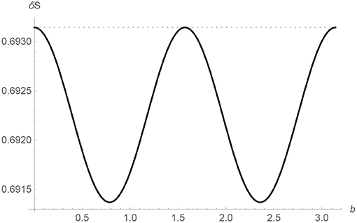
Figure 4. The curve represented by a thin line is the entropy jump δS as a function of b in Planck units for γ = μ = Δ = 1. The small bℓ_p behavior in (93) is apparent. The entropy is periodic for bℓ_p ∈ [0, π] as expected from (86). The dotted line represents the maximum possible entropy which is log[2] in our model.

3. Quantum Cosmology on a Superposition of Backgrounds

In the first part of this paper, we have seen how the fact that the Hilbert space of loop quantum cosmology is vastly larger than the standard Schrodinger representation implies (via coarse graining) that the coarse-graining entropy would rise generically through the evolution across the big bang would-be-singularity. In this section, we explore another closely related feature that leads to an apparent non-unitary evolution when dynamics are probed by a low-energy agent. The quantum dynamics in loop quantum cosmology depend on a UV regulator known as the area-gap Δ (section 2.1). We will see here that the loop quantum cosmology model can be extended naturally to admit superpositions of dynamics with different regulators. Such an extension generally leads to the dynamical development of correlations between the macroscopic and the microscopic degrees of freedom. If the microscopic degrees of freedom are assumed to remain hidden to low-energy observers, then such correlations lead to an apparent violation of unitarity in the low-energy description where pure states evolve into mixed states. In other words, the UV data needed to define the quantum dynamics open an independent microscopic channel for information to be degraded.

3.1. The UV Input in Quantum Cosmology: Revisiting the $\overline{\mu }$ Scheme

The $\stackrel{-}{\mu }$ scheme was designed to avoid an inconsistency in an early model of loop quantum cosmology with the low-energy limit (or large universe limit) of loop quantum cosmology (Green and Unruh, 2004). The problem arises from the effective compactification of the connection variable c due to the polymer regularization of the Hamiltonian with a fixed fiducial scale μ which implies that c and c + 4π/μ are dynamically identified. This leads to anomalous deviations from classical behavior in situations where the variable c is classically expected to be unbounded for large universes. This can be seen clearly in the present situation where the unimodular Hamiltonian (17) is given, in (c, p) variables, by

$\begin{array}{ll}H=\frac{3V_0}{8\pi G}\frac{c^2}{{\gamma }^2|p|}.& (51)\end{array}$

For non-vanishing energies (or equivalently non-vanishing cosmological constants), the conservation of the Hamiltonian implies that c grows as |p| ∝ a², i.e., c grows without limits as the universe expands so that no matter how small μ is, anomalous effects due to the compactification of the c become relevant at macroscopic scales (Noui et al., 2005). As no quantum gravity effects seem acceptable in the large universe regime for a model with finitely many degrees of freedom, this anomaly is seen as an inconsistency of the model.

The $\stackrel{-}{\mu }$ scheme solves this inconsistency by “renormalizing” the regulating scale μ as the universe grows (Equation 20). The interesting thing is that such a renormalization is justified by quantum geometry arguments that link the mini superspace model of loop quantum cosmology to the geometry of a microscopic background state in the full theory. The argument explicitly uses the idea that the low-energy degrees of freedom (dynamical variable of loop quantum cosmology) arise from the coarse graining of the fundamental ones in loop quantum gravity.

Here we review the construction of the $\stackrel{-}{\mu }$ scheme as described in Ashtekar and Singh (2011). Consider a fundamental quantum geometry state |s〉 in the Hilbert space of loop quantum gravity, representing a microscopic state on top of which the quantum cosmological coarse-grained dynamics will eventually be defined. Such an underlying fundamental state will have to be approximately homogeneous and isotropic up to a scale of L > ℓ_p with respect to the preferred foliation defining the comoving FLRW observers at low energies. If that is the case then such space slices can be divided into (approximately) cubic 3-cells of physical side length L which all have approximately equivalent quantum geometries. The area of a face of such cubic cells in Planck units will be denoted Δ_s so that $L^2={\ell }_p^2{\Delta }_s$. Note that Δ_s is a property of the underlying microstate: an area eigenstate if the microstate is an eigenstate, or an area expectation value if the state is sufficiently peaked on a quantum geometry and has small fluctuations around it. A simple realization is the one where Δ_s is an area eigenvalue, and the important assumption is that Δ_s is the same for all cells (this encodes the homogeneity of the microscopic state). Consider the area of a large two-dimensional surface (the face of a fiducial cell V), whose area is measured by the low-energy (coarse-grained) quantity p used as the configuration variable in loop quantum cosmology. We naturally would expect that $|p|\gg {\ell }_p^2$ or alternatively that

$\begin{array}{ll}N{\ell }_p^2{\Delta }_s=|p|,& (52)\end{array}$

where N denotes the number of microscopic cells contained in the coarse-grained surface (a face of V), and N ≫ 1. The fiducial cell has a fiducial coordinate volume V₀ and hence fiducial side coordinate length $V_0^{1/3}$. Therefore, the fiducial coordinate length $\stackrel{-}{\mu }$ of the microscopic homogeneity cells is given by the relation

$\begin{array}{ll}N{(\stackrel{-}{\mu }{V}_0^{1/3})}^2=V_0^{2/3}.& (53)\end{array}$

Combining the previous two equations, one recovers Equation (20), namely

$\begin{array}{ll}{\stackrel{-}{\mu }}_s^2\equiv {\stackrel{-}{\mu }}^2=\frac{{\ell }_p^2{\Delta }_s}{|p|},& (54)\end{array}$

i.e., the fiducial scale $\stackrel{-}{\mu }$ is dynamical: as the universe grows (and |p| becomes larger), the underlying fiducial length scale decreases. The fiducial regularization scale (53) depends on the fundamental state |s〉 via the quantity Δ_s, hence we denote it as ${\stackrel{-}{\mu }}_s$. When such a dynamical scale is used in the regularization of the quantum cosmology Hamiltonian, the effective compactification scale for c grows like |p| and the inconsistency previously discussed is avoided. This is transparent in terms of the new canonical pair (b, v). From Equation (15), we can see that $b=c{\stackrel{-}{\mu }}_s/(\sqrt{{\Delta }_s}{\ell }_p)$, in contrast with c (see 17), remains constant (see 51) in the de Sitter universe. The quantization of the Hamiltonian presented in section 2.1 introduces an effective compactification of the variable b whose dynamical effect is now only relevant when the cosmological constant approaches one in Planck units. This can be seen from (21). The cosmological constant is bounded from above by its natural value in Planck units due to the underlying quantum geometry structure while the anomalous IR behavior is avoided (the problems exhibited in the model studied in Green and Unruh, 2004 are also resolved).

The above is the standard account of the motivation of the $\stackrel{-}{\mu }$ scheme of Ashtekar et al. (2006) with the little twist (which is very important for us here) that Δ_s need not be the lowest area eigenvalue of loop quantum gravity. In the usual argument, the microscopic state is thought to be built from a special homogeneous spin network (geometry eigenstate) with all spins equal to the fundamental representation. This implies that, in the above construction, ${\Delta }_s={\Delta }_{1/2}\equiv 2\pi \gamma \sqrt{3}$. The observation here is that Δ_s can take different values according to the microscopic properties of the underlying quantum geometry state. One could take for instance all spins equal to the vector representation and then have ${\Delta }_s={\Delta }_1\equiv 4\pi \gamma \sqrt{2}$ instead, or take j as arbitrary and use Δ_s = Δ_j. It is important to point out that such a possibility can arise naturally in quantum cosmology models obtained in the group field theory framework (Gielen et al., 2013; Oriti et al., 2016, 2017).

As we have seen in section 3.1, the field strength regularization, and hence the Hamiltonian, depend on the value Δ_s of the background (approximately homogeneous) spin network state |s〉 through the dynamical scale ${\stackrel{-}{\mu }}_s$. In this way, the dynamics of loop quantum cosmology establish correlations with a microscopic degree of freedom in the underlying loop quantum gravity fundamental state. As such a degree of freedom (the area eigenvalue Δ_s of the minimal homogeneity cells) is quantum, it is natural to model the system by a tensor product Hilbert space ${H}$ ≡ ${H}$_m ⊗ ${H}$_lqc, where ${H}$_m is the Hilbert space representing the microscopic degree of freedom encoded in the minimal homogeneous cell operator (whose eigenvalues we denote as Δ_s), and ${H}$_lqc the standard kinematical Hilbert space of loop quantum cosmology.

General states in ${H}$ can be expressed as linear combinations of product states |s〉 ⊗ ψ in the respective factor Hilbert spaces. The quantum Hamiltonian has a natural definition on such states and therefore on the whole of ${H}$, namely

$\begin{array}{ll}\widehat{H}⊳(|s\rangle \otimes \psi )=|s\rangle \otimes {\widehat{H}}_{{\Delta }_s}⊳\psi ,& (55)\end{array}$

where Ĥ_Δs is the usual loop quantum cosmology Hamiltonian in the ${\stackrel{-}{\mu }}_s$ scheme, which in our particular case is defined in Equation (21) with regulator Δ = Δ_s.

Notice that the previous extension of the standard loop quantum cosmology framework to the larger Hilbert space ${H}$ is also natural from the perspective of the full theory. Indeed, the generally accepted regularization procedure of the Hamiltonian constraint in loop quantum gravity (first introduced by Thiemann, 1998 and further developed in recent analysis—see Ashtekar and Pullin, 2017 and references therein) is state dependent in that the loops defining the regulated curvature of the connection are added on specific nodes of the state where the Hamiltonian is acting upon. This feature finds its analog in the action (55) where the regulating scale Δ_s depends on the state |s〉 ∈ ${H}$_m.

In order to simplify the following discussion we will restrict states in ${H}$_m even further and consider a subspace 𝔥 = ℂ² ⊂ ${H}$_m, i.e., we will model the situation where the underlying microscopic state is an arbitrary superposition of only two fixed microscopic homogeneous spin-network states. For example we take

$\begin{array}{ll}h\equiv \text{span}\left[|+\rangle ,|-\rangle \right],& (56)\end{array}$

where |±〉 ∈ ${H}$_m are two suitable orthogonal background states (these two states will be conveniently picked below). From the infinitely dimensional Hilbert space ${H}$_m we are now selecting a single q-bit subspace ℂ². The Hilbert space of our model is

$\begin{array}{ll}{H}=𝔥\otimes {{H}}_{\text{lqc}}.& (57)\end{array}$

The factor 𝔥 represents additional microscopic (hidden to low-energy observers) UV degrees of freedom, while ${H}$_lqc encodes the data that under suitable circumstances (e.g., when the universe is large) represent the low-energy cosmological degrees of freedom.

In this way we see that in addition to the intrinsic degeneracy of energy eigenvalues analyzed in the first part of this paper, there is another candidate for the microscopic degree of freedom associated with the regularization of the Hamiltonian action via the $\stackrel{-}{\mu }$-scheme. Both mechanisms are correct for the present loop quantum cosmology toy model but reflect generic properties of the full theory of loop quantum gravity. More generally, we expect similar features to be present in any quantum gravity approach where smooth geometry is only emergent from a discrete fundamental theory.

From now on we adopt the convenient notation |s〉 with s = ± for such preferred basis elements of 𝔥. With this notation, and using (21), the Hamiltonian (55) becomes

$\begin{array}{l}{\widehat{H}}_0⊳(|s\rangle \otimes |\psi \rangle )=\frac{3V_0}{8\pi G{\gamma }^2}\frac{1}{{\Delta }_s{\ell }_p^2}\left(\sin {(\sqrt{{\Delta }_s}{\ell }_{p}b)}^2\right)⊳|s\rangle \otimes |\psi \rangle \\ =-\frac{3V_0}{8\pi G{\gamma }^2}{\displaystyle \sum _{\nu }\frac{1}{2{\Delta }_s{\ell }_p^2}}|s\rangle \otimes |v\rangle [\Psi (v\\ -4\sqrt{{\Delta }_s}{\ell }_p)+\Psi (\nu +4\sqrt{{\Delta }_s}{\ell }_p)-2\Psi (\nu )],& (58)\end{array}$

where Ψ(ν)≡〈ν|ψ〉.

Now, the only special feature of the basis |±〉 is that it is preferred from the perspective of the regularization of the effective (unimodular) loop quantum cosmology Hamiltonian. Consequently, a natural question for the quantum theory is how the dynamics would look if the initial state is arbitrary in factor 𝔥? More precisely, what if we consider the linear combination of two background spin networks $\frac{1}{\sqrt{2}}(|+\rangle +|-\rangle )\in \mathfrak{h}$ times a loop quantum cosmology wave function as depicted in Figure 5? To answer this question we consider a special initial state where correlations between the low-energy and the UV degrees of freedom are not present. This will lead to a reduced density matrix—tracing out the microscopic space 𝔥 in (57)—that is pure initially, the form of such a state is illustrated in Figure 5. At the same time we want to be able to diagonalize the Hamiltonian with such uncorrelated initial states; more precisely this boils down to diagonalizing both H_Δ+ and H_Δ− in ${H}$_lqc. This implies that the factor ψ(ν) ∈ ${H}$_lqc, in Figure 5, must be supported on a lattice ${\Gamma }_{\Delta }^{ϵ}$ that is left invariant by the action of both H_Δ+ and H_Δ− (left invariant in the sense that the shift operators in the definition of the Hamiltonian only relate to points of ${\Gamma }_{\Delta }^{ϵ}$ and never map points out). This can be achieved by assuming that $\sqrt{{\Delta }_{+}}=m\sqrt{{\Delta }_{-}}$ for some natural number m. For simplicity we will take m = 2 from now on¹¹. The parameter ϵ will be taken so that the lattice ${\Gamma }_{\Delta }^{ϵ}$ contains the point ν = 0. This is a standard choice. With all this, the invariant lattice, denoted as Γ_Δ−, is

$\begin{array}{ll}{\Gamma }_{{\Delta }_{-}}\equiv {\Gamma }_{k=2{\sqrt{\Delta }}_{-}{\ell }_p}^{ϵ=0}.& (59)\end{array}$

Note that in the notation described below (37), we have that Γ_Δ− = Γ₁ ∪ Γ₂.

FIGURE 5

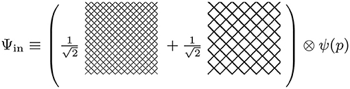
Figure 5. Schematic representation of the state of interest. There are two different UV structures with dynamical implications via the $\stackrel{-}{\mu }$ scheme. The state represented here has trivial correlations with the microscopic structure and would lead to a zero initial entanglement entropy state as defined by the reduced density matrix where the background state is traced out.

The choices made above are not mandatory. One could have chosen a different initial state. The previous choice is particularly interesting here because it would lead to a reduced initial density matrix that is pure and hence initially had vanishing entanglement entropy. Other states would involve correlations and would therefore carry a non vanishing entropy load from the beginning. For the discussion that interests us here and for the analogy with black hole evaporation, it is more transparent to set the entropy to zero initially.

An arbitrary (unimodular) loop quantum cosmology state associated with such a choice of background state can be expressed as:

$\begin{array}{l}{\Psi }_{\text{in}}(\nu ,t)=\langle \nu |\frac{1}{\sqrt{2}}{\displaystyle \sum _s|s\text{〉 }\otimes |{\Psi }_{\text{in}}(t)\rangle }\\ =\frac{1}{\sqrt{2}}{\displaystyle \sum _s|s\otimes [{\delta }_{{\Gamma }_{{\Delta }_{-}}}(\nu )}\\ {\displaystyle \underset{0}{\overset{\frac{\pi }{\sqrt{{\Delta }_{-}}{\ell }_p}}{\int }}d}k\psi (k;b_0,{\nu }_0)\exp (-i{E}_s(k)t)]& (60)\end{array}$

where ψ(k; b₀, ν₀) is a properly normalized function peaked at k = b₀ and ν = ν₀. The initial state in the momentum representation is given by:

$\begin{array}{l}{\Psi }_{\text{in}}(b,t)={\displaystyle \sum _{\nu \in {\Gamma }_{{\Delta }_{-}}^0}\langle b,1\cup 2|\nu \rangle }\langle \nu |{\Psi }_{\text{in}}(t)\rangle \\ =\frac{\pi }{\sqrt{{\Delta }_{-}}{\ell }_p}{\displaystyle \sum _s|s\rangle }\otimes \psi (b;b_0,{\nu }_0)e^{-i{E}_s(b)t}& (61)\end{array}$

Where, in the first line, we used the natural extension of the notation introduced in (37) where |b, 1 ∪ 2〉 means an eigenstate of the corresponding shift operators (19) supported on the lattice Γ_Δ− = Γ₁ ∪ Γ₂. Notice that we can also write

$\begin{array}{ll}|b,1\cup 2\rangle =|b,1\rangle +|b,2\rangle ,& (62)\end{array}$

keeping in mind that terms on the r.h.s. are individually eigenstates of the shift operators with twice the lattice spacing of Γ_Δ−. We also used

$\begin{array}{ll}{\displaystyle \sum _{\nu \in {\Gamma }_{{\Delta }_{-}}^0}}exp\left(i\frac{b-k}{2}\nu \right)=\frac{\pi }{\sqrt{{\Delta }_{-}}{\ell }_p}\delta (b-k).& (63)\end{array}$

We can then write

$\begin{array}{ll}{\Psi }_{\text{in}}(t)={{\displaystyle \sum _s}}^{}{{\displaystyle \int }}^{}\text{D}b|s\rangle \otimes |b,1\cup 2\rangle \psi (b;b_0,{\nu }_0)e^{-i{E}_s(b)t},& (64)\end{array}$

where

$\begin{array}{ll}\text{D}b\equiv \frac{\pi }{\sqrt{2{\Delta }_{-}}{\ell }_p}db,& (65)\end{array}$

is the Haar measure on the circle of circumference $\pi /\sqrt{2{\Delta }_{-}}{\ell }_p$. We notice from (64) that even when our initial state contains no correlations between the low energy degrees of freedom represented by b and the microscopic degrees of freedom encoded in |s〉 at t = 0, quantum correlations between the two will develop with time due to the non trivial dependence of the energy spectrum with s. Even when this is quite clear from (64), one can state this fact in an equivalent way by analysing the (pure) density matrix ρ_in(t) ≡ |Ψ_in(t)〉〈Ψ_in(t)|, whose matrix elements in the b basis are:

$\begin{array}{l}{\rho }_{\text{in}}(t)\equiv {\displaystyle \sum _{s,s^{\prime }}{\displaystyle \int \text{D}}}b\text{ D}{b}^{\prime }\left(\overline{\psi }(b;b_0,{\nu }_0)\psi (b^{\prime };b_0,{\nu }_0)e^{i[E_s(b)-E_{s^{\prime }}(b^{\prime })]t}\right)\\ \times |b^{\prime },1\cup 2\rangle |s^{\prime }\rangle |b,1\cup 2\rangle |s\rangle .& (66)\end{array}$

As coarse-grained observers are assumed to be insensitive to the microscopic structure encoded here in the “spin” quantum number s, low-energy physical information is encoded in the reduced density matrix

$\begin{array}{l}{\rho }_{\text{inR}}(t)\equiv {\displaystyle \sum _s{\displaystyle \int \text{D}}}b\text{ D}{b}^{\prime }(\overline{\psi }(b;b_0,{\nu }_0)\psi (b^{\prime };b_0,{\nu }_0)\\ e^{i[E_s(b)-E_s(b^{\prime })]t})& (67)\end{array}$

$\begin{array}{ll}\times |b^{\prime },1\cup 2\rangle |s\text{'}\rangle |b,1\cup 2\rangle |s\rangle ,& (68)\end{array}$

which can be simply be written as

$\begin{array}{ll}{\rho }_{\text{inR}}\text{(}t)=\frac{1}{2}{{\displaystyle \sum _s}}^{}s|{\Psi }_s(t)\rangle \langle {\Psi }_s(t)|& (69)\end{array}$

where

$\begin{array}{ll}|{\Psi }_s(t)\rangle \equiv {{\displaystyle \int }}^{}\text{ D}b\psi (b;b_0,{\nu }_0)e^{-i{E}_s(b)t}|b,1\cup 2\rangle .& (70)\end{array}$

Notice that (69) is only pure at t = 0 and becomes mixed due to the correlations evoked above as time passes. One can compute the entanglement entropy S(t) ≡ −Tr[ρ_inR(t)log(ρ_inR(t))] which turns out to be given by the simple analytic expression (see Appendix A)

$\begin{array}{ll}S(t)=-log\left(1-\frac{\delta }{2}\right)-\frac{\delta }{2}log\left(\frac{\delta }{1-\frac{\delta }{2}}\right),& (71)\end{array}$

where

$\begin{array}{ll}\delta (t)\equiv 1-{\displaystyle |\int \text{D}b\overline{\psi }(b;b_0,{\nu }_0)\psi (b;b_0,{\nu }_0)e^{i\left[E_{+}(b)-E_{-}(b)\right]t}|.}& (72)\end{array}$

For generic wave packets ψ_s(b), the entanglement entropy is a monotonic growing function of time which grows asymptotically to the maximally mixed situation S_max = log(2) (see an example in Figure 6).

FIGURE 6

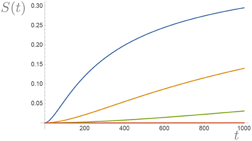
Figure 6. Here we plot S(t) as a function of time for a Gaussian wave packet centered at b = 2.5 10⁻², b = 5 10⁻², b = 7 10⁻², and b = 10⁻¹ with width σ = b, respectively. Numerical integration plus the approximation (73) was used with the assumption that $2({\Delta }_{+}-{\Delta }_{-})/{\gamma }^2=1$, all in Planck units. As b grows the scalar curvature (the cosmological constant) grows and the rate at which entropy increases grows as well. For b ≪ 1, an effective unitary evolution is recovered.

FIGURE 7

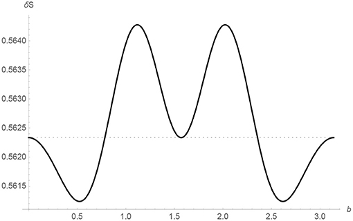
Figure 7. The entropy jump δS as a function of b in Planck units for γ = μ = Δ₋ = 1. The small bℓ_p behavior in (93) is apparent. The entropy is periodic for bℓ_p ∈ [0, π] as expected from (86).

A more intuitive picture can be obtained from a suitable expansion of the energy eigenvalues (24) in powers of the label bℓ_p

$\begin{array}{l}\begin{array}{c}{E}_s(b)=\frac{3V_0}{8\pi G{\gamma }^2}\frac{1}{{\Delta }_s{\ell }_p^2}{(\sin (\sqrt{{\Delta }_s}{\ell }_{p}b))}^2\end{array}\\ =\frac{3V_0}{8\pi G{\gamma }^2}{b}^2-\frac{V_0}{8\pi G{\gamma }^2}{\Delta }_s{\ell }_p^2{b}^4+b^{2}O({\ell }_p^4{b}^4).& (73)\end{array}$

Such an expansion makes sense in that it allows for the identification of the low energy effective Hamiltonian (the one that one would define in a purely Wheeler-DeWitt quantization) plus corrections that involve interactions with the underlying discrete structure of LQG here represented by the spin s degree of freedom. Namely, we can read from the previous expansion that

$\begin{array}{ll}{H}_{\text{eff}}\equiv H_{\text{eff}}^0(b)+\Delta H(b,s),& (74)\end{array}$

where ${\widehat{H}}_{\text{eff}}^0(\widehat{b})\equiv \frac{6}{{\gamma }^2}{\widehat{b}}^2$ is the Wheeler-DeWitt Hamiltonian and the additional term is an interaction with the environment represented by the underlying discrete structure represented by the dependence on s (a hidden degree of freedom from the low-energy continuum perspective). Of course, the hats in the previous equation denote operators in a different representation (the continuum Schrodinger representation) that is not unitarily equivalent to the “fundamental” polymer representation introduced in section 2.1 and used in the LQC setup (recall for instance that the operator $\widehat{b}$ does not even exist in the polymer representation).

The lack of purity for t > 0 of the reduced density matrix (69) is due to correlations that develop between the low-energy degree of freedom b and the hidden microscopic degree of freedom s via this non trivial interaction Hamiltonian. This means that generically [i.e., for arbitrary initial states ψ_s(b)], the fundamental evolution would seem to violate unitarity, from the perspective of low-energy observers, due to the decoherence with the microscopic quantum geometric structure. Notice however that for states ψ_s(b) picked at sufficiently small $\stackrel{-}{k}$, i.e., $\stackrel{-}{k}\sqrt{{\Delta }_s}{\ell }_p\ll 1$, we have from (22) that

$\begin{array}{ll}\Lambda (b)\approx 3{\gamma }^{-2}{b}^2& (75)\end{array}$

and the density matrix (69) is pure at all times.

More precisely, we can translate the criterion for the absence of decoherence with the underlying microscopic discrete structure in terms of the value of the cosmological constant of the given state. For an eigenstate of the Hamiltonian the relation is given by Λ ≡ E_s(b). Therefore the criterion for the absence of decoherence in terms of the cosmological constant is

$\begin{array}{ll}{\Delta }_s{\ell }_p^2{\gamma }^2\Lambda \approx {\ell }_p^2\Lambda \ll 1& (76)\end{array}$

Interestingly, for states with low values of the cosmological constant in natural units—equivalent semi-classically to the scalar curvature R in our matter-free model—define a decoherence free subspace. When the cosmological constant does not satisfy condition (76), decoherence with the microscopic structure is turned on and maximized for Λ of order one in Planck units: notice incidentally that due to the polymer quantization the cosmological constant is bounded by

$\begin{array}{ll}{\Lambda }_{\text{max}}=\frac{3}{{\gamma }^2{\Delta }_{\frac{1}{2}}{\ell }_p^2}.& (77)\end{array}$

For low values of Λ, unitarity is recovered in the effective description that ignores the microscopic structure.

Decoherence takes place here due to an interaction between the low-energy coarse degrees of freedom and the microscopic discreteness in the underlying quantum geometry background, but in a way (in our simple model) that the energy and hence the cosmological constant is conserved. However, the presence of decoherence suggests the possibility for a natural deviation of this idealized absence of dissipation: generally decoherence and dissipation often come together. Therefore, a surprising and unexpected consequence of our analysis is the suggestion of a natural channel for the relaxation of a large cosmological constant due to the possibility of dissipative effects associated with the decoherence pointed out here.

Incidentally, all this shows that only in the limit of low values of E (small cosmological constant), the coarse graining that leads from the full theory of loop quantum gravity to the mini superspace description of loop quantum cosmology is well-defined. This is not surprising and only confirms the usual intuition that drives the construction of models of loop quantum cosmology. However, it opens the door for a qualitative understanding of the necessity of decoherence effects in more general situations. For instance, the standard ${\stackrel{-}{\mu }}_s$ construction suggests that coarse graining is weaker at the big bang where the Hamiltonian evolution (58) takes the universe through the ν = 0 states. During this high (spacial) curvature phase it is natural to expect that the higher corrections in (73) (describing the interaction with the microscopic Planckian structure) can no longer be neglected.

Interestingly, there is another way to make decoherence disappear. This is due to the asymptotic behavior of the separation of area eigenvalues in loop quantum gravity which imply that for large Δ_s there are states such that ${\Delta }_s-{\Delta }_{s^{\prime }}\approx {\Delta }_{s}exp(-\pi \sqrt{2{\Delta }_s/3})$ (Fernando Barbero et al., 2018). Therefore, in the continuum limit ${\Delta }_s-{\Delta }_{s^{\prime }}\ll 1$ the dynamical entanglement growth of our model can be made as small as wanted.

3.2. Matter Coupling Produces an Entanglement Entropy Jump at the Big Bang

In the pure gravity case, we can make decoherence as small as needed by choosing states with a cosmological constant that is sufficiently small. Here we show that this is no longer possible once matter is added and that there is a generic development of correlations with the UV degrees of freedom in the evolution across the would-be-singularity: an initially pure state (reduced low-energy density matrix) evolves generically into a mixed state (reduced low-energy density matrix) after the big bang.

In order to see this in more detail, we just need to write out the matter Hamiltonians acting in the Hilbert space (57). One needs the natural generalization of the expressions written in section 2.3 for the present context. For instance, for scalar field coupling, Equation (32) becomes

$\begin{array}{ll}{\widehat{H}}_{\varphi }⊳(|s\rangle \otimes |\psi \rangle )=-m{\displaystyle \sum _{\nu \in \Gamma }|s\rangle \otimes |\nu \rangle h_{\varphi }(\nu ;\sqrt{{\Delta }_s}{\ell }_p)\Psi (\nu ,\varphi ),}& (78)\end{array}$

where

$\begin{array}{ll}{h}_{\varphi }(\nu ;\lambda )\equiv \frac{p_{\varphi }^2}{16{\lambda }^4}{\left(|\nu +2\lambda {|}^{\frac{1}{2}}-|\nu -2\lambda {|}^{\frac{1}{2}}\right)}^4.& (79)\end{array}$

The momentum p_ϕ commutes with the Hamiltonian and thus is a constant of motion. As before, if we consider an eigenstate of p_ϕ then the problem reduces again to a scattering problem with a potential decaying like 1/ν² when solving the time-independent Schrodinger equation

$\begin{array}{ll}{\widehat{H}}_0+{\widehat{H}}_{\varphi }⊳(|s\rangle \otimes |\psi \rangle )=E(|s\rangle \otimes |\psi \rangle ).& (80)\end{array}$

From the discussion in section 2.3, we can capture the basic qualitative effect of matter interaction by considering a simple solvable model where the matter contribution is concentrated at a single event at the big bang. None of the qualitative conclusions that follow depend on this simplification, and a more realistic free scalar field model can be dealt with (some results are shown in Appendix D). With some extra effort one could actually analyze a more realistic model [say the one defined by (78)] but the conclusion will remain the same. Therefore, we consider

$\begin{array}{ll}\widehat{H}={\widehat{H}}_0+\mu {\widehat{H}}_{\text{int}},& (81)\end{array}$

where μ is a dimensionless coupling, Ĥ₀ is given in (58), and Ĥ_int is the generalization of (36)

$\begin{array}{ll}{\widehat{H}}_{\text{int}}⊳(|s\rangle \otimes |\psi \rangle )\equiv {{\displaystyle \sum _v}}^{}\widehat{O}|s\rangle \otimes |\nu \rangle \frac{{\delta }_{\nu ,0}}{\sqrt{{\Delta }_s}}\Psi (0)& (82)\end{array}$

where Ô is a self adjoint operator in 𝔥 = ℂ². A natural and simple model for this operator is to choose

$\begin{array}{ll}\widehat{O}\equiv {\ell }_p^{-4}\frac{V_0}{\sqrt{{\Delta }_s}}.& (83)\end{array}$

This choice is formulated in the notation introduced below (58) and inspired by the analogy with a spin system. We have added by hand an interaction Hamiltonian that switches on only when the universe evolves through the would-be-singularity at the zero volume state. This encodes the idea of the intrinsic uncertainty of the peculiar construction of the mini superspace model of loop quantum cosmology that we discussed in section 3.1. The discrete local degrees of freedom must be important close to the big bang and symmetry reduction must fail in some way that can only be correctly described if a full quantum gravity theory is available. Here we model such unknown dynamics in the simplest fashion available to us here, which consists of including the possibility for the background state |s〉 (representing in spirit the underlying quantum geometry) to be modified by the dynamics via Ĥ_int.

Here we proceed as in section 2.4 while keeping in mind that, in the present case, there are two distinct cases at hand given by the two possible values Δ_±. Let us consider an in-state of the form

$\begin{array}{ll}|k,s\rangle =|s\rangle \otimes |\nu \rangle \{\begin{array}{cc}{e}^{-i\frac{k}{2}\nu }+A_s(k)e^{i\frac{k}{2}\nu }& \text{(}\nu \ge 0\text{)}\\ B_s(k)e^{-i\frac{k}{2}\nu }& (\nu \le 0),\end{array}& (84)\end{array}$

where A_s(k) and B_s(k) are coefficients depending on k and (in contrast with the case in section 2.4) now also on s = ±1 (with |±〉 the eigenstates of Ŝ_z). For suitable coefficients, such states are eigenstates of the Hamiltonian H₀ as well as the full Hamiltonian (35). Arbitrary solutions (wave packets) can then be constructed in terms of appropriate superpositions of these “plane-wave” states.

$\begin{array}{l}\begin{array}{c}{A}_s(k)=\frac{-i{\Theta }_s(k)}{1+i{\Theta }_s(k)}\end{array}\\ \begin{array}{c}{B}_s(k)=\frac{1}{1+i{\Theta }_s(k)}\end{array}& (85)\end{array}$

where

$\begin{array}{ll}{\Theta }_s(k)\equiv \frac{16\pi {\gamma }^2}{3}\frac{\mu }{sin(2k\sqrt{{\Delta }_s}{\ell }_p)}.& (86)\end{array}$

One can superimpose the previous eigenstates to produce wave packets (semiclassical states) for the wave function of the universe that are picked at value ν₀ of the rescaled volume (see footnote 6). Wave packets will evolve in time according to the Schrodinger equation which in our case is just a discrete analog of the one corresponding to a free particle in quantum mechanics with an interaction term at the “origin” ν = 0. If we start with a state that is sufficiently picked around ν₀ for ν ≫ ℓ_p initially, then the state can be described in terms of the superposition (64) where the explicit values of the coefficients A_s(b) and B_s(b) do not appear. Equation (42) is generalized to

$\begin{array}{l}\begin{array}{c}\begin{array}{l}{\Psi }_{\text{in}}(t\ll 0)={\displaystyle \int Db(|b,1\rangle \psi (b;b_0,{\nu }_0)}\\ +|b,2\rangle \psi (b;b_0,{\nu }_0))e^{-i{E}_{-}(b)t}\end{array}\end{array}\\ +{\displaystyle \int \text{D}}b(|b,1\rangle \psi (b;b_0,{\nu }_0)+|b,2\rangle \psi (b;b_0,{\nu }_0))e^{-i{E}_{+}(b)t}.& (87)\end{array}$

The coefficients (85) enter the expression of the scattered wave packet at a later time which becomes

$\begin{array}{l}{\Psi }_{\text{out}}(t\gg 0)=\\ {\displaystyle \int \text{D}}b|-\rangle \otimes |b,1\cup 2\rangle [\psi (-b;b_0,{\nu }_0)A_{-}(-b)\\ +;\psi (b;b_0,{\nu }_0)B_{-}(b)]e^{-i{E}_{-}(b)t}+\\ {\displaystyle \int \text{D}}b|+\rangle \otimes [|b,1\rangle (\psi (-b;b_0,{\nu }_0)A_{+;}(-b)\\ +;\psi (b;b_0,{\nu }_0)B_{+;}(b))+|b,2\rangle \psi (b;b_0,{\nu }_0)]e^{-i{E}_{+;}(b)t}.& (88)\end{array}$

Note that the solution of the scattering problem for the E₊(b) eigenvalues is asymmetric with respect to the components of the in-state supported on Γ₁ and Γ₂. Indeed the states |b, 2〉 are eigenstates of the Hamiltonian directly because they are not supported on ν = 0 and hence they do not “see” the interaction: this is captured by trivial scattering coefficients for this component.

3.3. Entropy Associated With the Entanglement With the UV Degrees of Freedom

From the previous initial state we can calculate [by tracing over the factor 𝔥, see (57)] the initial reduced density matrix

$\begin{array}{ll}\begin{array}{l}{\rho }_{\text{in}}^R(t)={\displaystyle \int \text{D}}b\text{ D}b\prime e^{i[E_{+}(b)-E_{+}(b^{\prime })]t}\\ \times [|b^{\prime },1\rangle \psi (b\prime ;b_0,{\nu }_0)+|b^{\prime },2\rangle \psi (b\prime ;b_0,{\nu }_0)]\\ \left[\langle b,1|\overline{\psi }(b;b_0,{\nu }_0)+\langle b,2|\overline{\psi }(b;b_0,{\nu }_0)\right]\\ +{\displaystyle \int \text{D}}b\text{ D}b\prime e^{i[E_{-}(b)-E_{-}(b^{\prime })]t}\\ \times [|b^{\prime },1\rangle \psi (b\prime ;b_0,{\nu }_0)+|b^{\prime },2\rangle \psi (b\prime ;b_0,{\nu }_0)]\\ [\langle b,1|\overline{\psi }(b;b_0,{\nu }_0)+\langle b,2|\overline{\psi }(b;b_0,{\nu }_0)].\end{array}& (89)\end{array}$

The reduced density matrix after the big bang is

$\begin{array}{l}{\rho }_{\text{out}}^{\text{R}}(t)={\displaystyle \int \text{D}}b\text{ D}{b}^{\prime }{e}^{i[E_{+}(b)-E_{+}(b^{\prime })]t}\\ [\langle b,1|(\overline{\psi }(-b;b_0,{\nu }_0){\overline{A}}_{+}(-b)+\overline{\psi }(b;b_0,{\nu }_0){\overline{B}}_{+}(b))\\ +\langle b,2|\overline{\psi }(b;b_0,{\nu }_0)]\\ [|b,1\rangle \left(\psi (-b^{\prime };b_0,{\nu }_0)A_{+}(-b^{\prime })+\psi (b^{\prime };b_0,{\nu }_0)B_{+}(b^{\prime })\right)\\ +|b,2\rangle \overline{\psi }(b^{\prime };b_0,{\nu }_0)]+\\ e^{i[E_{-}(b)-E_{-}(b^{\prime })]t}[|b^{\prime },1\cup 2\rangle \psi (-b^{\prime };b_0,{\nu }_0)A_{-}(-b^{\prime })\\ +|b^{\prime },1\cup 2\rangle \psi (b^{\prime };b_0,{\nu }_0)B_{-}(b^{\prime })\\ \times [\langle b,1\cup 2|\overline{\psi }(-b;b_0,{\nu }_0){\overline{A}}_{-}(-b)\\ +\langle b,1\cup 2|\overline{\psi }(b;b_0,{\nu }_0){\overline{B}}_{-}(b)],& (90)\end{array}$

where α₊ = 1/4 and α₋ = 1 and δ_s+ is unity when s = + and vanishes when s = −. Then the non vanishing entries of the reduced density matrix are

$\begin{array}{l}{\rho }_{out}^{R11}(b_0,b_0)=\frac{1}{4}\left(|B_{+}(b_0){|}^2+|B_{-}(b_0){|}^2\right)\\ {\rho }_{out}^{22}(b_0,b_0)=\frac{1}{4}\left(1+|B_{-}(b_0){|}^2\right)\\ {\rho }_{out}^{R12}(b_0,b_0)=\frac{1}{4}\left(B_{+}(b_0)+|B_{-}(b_0){|}^2\right)=\overline{{\rho }_{out}^{R21}(b_0,b_0)}\\ {\rho }_{out}^{R11}(-b_0,-b_0)=\frac{1}{4}\left(|A_{+}(-b_0){|}^2+|A_{-}(-b_0){|}^2\right)\\ {\rho }_{out}^{R22}(-b_0,-b_0)=\frac{1}{4}\left(|A_{-}(-b_0){|}^2\right)\\ {\rho }_{out}^{R12}(-b_0,-b_0)=\frac{1}{4}\left(|A_{-}(-b_0){|}^2\right)\\ =\overline{{\rho }_{out}^{R21}(-b_0,-b_0)}\\ {\rho }_{out}^{R11}(b_0,-b_0)=\frac{1}{4}\left({\overline{A}}_{+}(-b_0)B_{+}(b_0)+{\overline{A}}_{-}(-b_0)B_{-}(b_0)\right)\\ =\overline{{\rho }_{out}^{R11}(-b_0,b_0)}\\ {\rho }_{out}^{R22}(b_0,-b_0)=\frac{1}{4}\left({\overline{A}}_{-}(-b_0)B_{-}(b_0)\right)=\overline{{\rho }_{out}^{R22}(-b_0,b_0)}\\ {\rho }_{out}^{R21}(b_0,-b_0)=\frac{1}{4}\left({\overline{A}}_{+}(-b_0)+{\overline{A}}_{-}(-b_0)B_{-}(b_0)\right)\\ =\overline{{\rho }_{out}^{R12}(-b_0,b_0)}\\ {\rho }_{out}^{R12}(b_0,-b_0)=\frac{1}{4}\left({\overline{A}}_{-}(-b_0)B_{-}(b_0)\right)=\overline{{\rho }_{out}^{R21}(-b_0,b_0)}.& (91)\end{array}$

The matrix ${\rho }_{out}^R$ is positive definite, $\text{Tr}\left[{\rho }_{out}^R\right]=1$ and ${\rho }_{out}^R={\rho }_{out}^{R†}$. In the case b₀ℓ_p ≪ 1 we have

$\begin{array}{ll}{\Theta }_s(b_0)\approx \frac{8\pi {\gamma }^2\mu }{3}\frac{1}{b_0\sqrt{{\Delta }_s}{\ell }_p}.& (92)\end{array}$

We can now compute the entanglement entropy jump δS to the first leading order in b₀ℓ_p/μ. The result [expressed in terms of the cosmological constant in this regime, namely (75)] is

$\begin{array}{ll}\delta S={\delta }_{0}S-\frac{3{\Delta }_{-}{\ell }_p^{2}log(3)}{128{\pi }^2{\gamma }^2{\mu }^2}\Lambda +{O}({\Lambda }^2{\ell }_p^4),& (93)\end{array}$

where ${\delta }_{0}S=2log(2)-\frac{3}{4}log(3)$. The previous equation shows that the entropy jump is non trivial at crossing the big bang would-be-singularity, even in the low cosmological (low-energy) limit where (according to the analysis of the previous section) decoherence with the microscopic Planckian structure can be neglected during the time the universe is large. Information is unavoidably degraded (it seems lost for low-energy observers) during the singularity crossing.

The general entropy jump for arbitrary (not necessarily small) Λ can be computed explicitly. Its value is bounded by log(2) in our model. Finally, the energy is conserved through the big bang and during all the dynamical evolutions for the arbitrary values of b₀. The decoherence and entanglement which can be interpreted as an information loss happens without energy spending as required by the scheme put forward in Perez (2015).

4. Discussion

We have seen that one can precisely realize the scenario put forward in Perez (2015) for the resolution of Hawking's information loss paradox in quantum gravity in the context of loop quantum cosmology. The key feature making this possible is the existence of additional degrees of freedom with no macroscopic interpretation which unavoidably entangle with the macroscopic degrees of freedom during the dynamical evolution and lead to a reduced density matrix whose entropy grows. The fundamental description is unitary but the effective description—that does not take the microscopic degrees of freedom into account and hence is analogous to the QFT description of BH evaporation—evolves pure states into mixed states. The microscopic degrees of freedom in the toy model are not introduced by hand, their existence is intimately related to the peculiar choice of representation of the fundamental phase space variables that leads to singularity resolution (Bojowald, 2001). Moreover, such a representation mimics the one used in the full theory of loop quantum gravity (Lewandowski et al., 2006) where also one expects such extra residual and microscopic degrees of freedom to exist and remain hidden to low-energy coarse-grained observers describing physics in terms of an effective QFT.

From a more general perspective, we expect this scenario to transcend the framework of loop quantum gravity: in any approach to quantum gravity, where spacetime geometry is emergent¹² from more fundamental discrete degrees of freedom, the effect (precisely illustrated here by our toy model) would generically occur.

These results extrapolated to the context of black hole formation and evaporation suggest a simple resolution of the information paradox that avoids the pathological features of other proposals. For instance, the possible development of firewalls (Almheiri et al., 2013; Braunstein et al., 2013) or the risks of information cloning that the holographic type of scenarios must deal with (Marolf, 2017) are completely absent here. As decoherence in our model takes place without diffusion Unruh (2012), the usual difficulties (Banks et al., 1984) with energy conservation in the purification process are avoided along the lines of Unruh and Wald (1995); Unruh (2012) in a concrete quantum gravity framework (hence without the problems faced by the QFT approach Hotta et al., 2015; Wald, 2019).

We notice that the possibility of decoherence illustrated in the present model also suggests the possibility of diffusion into the underlying Planckian structure, such diffusion might have, in suitable situations, important consequences at large scales as argued in a series of recent papers (Josset et al., 2017; Perez et al., 2018; Perez and Sudarsky, 2019). The present model is very simplistic and realizes an example where such diffusion is not possible due to (unimodular) energy conservation and the fact that the microscopic degrees of freedom do not contribute independently to the Hamiltonian. Nevertheless, one could generalize these models easily in order to include diffusion. This possibility is under current investigation and we plan to report the results elsewhere.

Data Availability Statement

The original contributions presented in the study are included in the article/Supplementary Material, further inquiries can be directed to the corresponding author/s.

Author's Note

This is a toy model of quantum cosmology that illustrates a novel mechanism for the resolution of Hawking's information puzzle for black hole evaporation.

Author Contributions

All authors listed have made a substantial, direct and intellectual contribution to the work, and approved it for publication.

Conflict of Interest

The authors declare that the research was conducted in the absence of any commercial or financial relationships that could be construed as a potential conflict of interest.

Acknowledgments

We thank P. Martin-Dussaud for finding for outlining useful inequalities in reference (Petz and Ohya, 1993). We thank M. Geiller, C. Rovelli, S. Speziale, M. Varadarajan, and E. Wilson-Ewing for their stimulating discussions and Pietro Donà for the key remark that the notion of coarse-graining entropy that we had initially in mind could be written as standard entanglement entropy. This manuscript has been released as a pre-print at [https://inspirehep.net/literature/1772094] (Perez et al.).

Supplementary Material

The Supplementary Material for this article can be found online at: https://www.frontiersin.org/articles/10.3389/fspas.2021.604047/full#supplementary-material

Footnotes

1. ^This is not the case in modifications of quantum mechanics where the collapse of the wave function happens spontaneously. In such theories information is actually destroyed (for a discussion of black hole evaporation in such contexts; see Modak et al., 2015; Okon and Sudarsky, 2017, 2018).

2. ^To these two specialty conditions one might also have to add one concerning the state of the hypothetical microscopic constituents at the Planck scale if the view we are advocating here and in Perez (2015, 2017) is correct.

3. ^In the Schwarzshild background, the frequency measured by a radially freely falling observer normal to the r=constant hypersurfaces goes like

$\begin{array}{ll}{\omega }^2(r)=\frac{{\ell }^2}{r^2}+\frac{r}{2M}{E}^2+{O}\left(\frac{r^2}{M^2}\right),& (3)\end{array}$

where E = −k · ξ and ℓ = k · ψ are the conserved quantities associated with the massless particle with wave vector k^a, and ξ^a and ψ^a are the stationarity and rotation killing fields of the background. The qualitative behavior approaching r = 0 would be the same for any other observer measuring ω (the divergence of ω is observer-independent). Only exactly spherically symmetric modes with ℓ = 0 would become IR at the singularity. However, this conclusion is no longer true if the BH rotates or if we consider that at the fundamental level, states with exact spherical symmetry inside the BH are of measure zero. Notice that such UV divergence in the non-spherically symmetric Hawking partners implies large deviations from spherical symmetry near the singularity (if their back reaction would be taken into account). This should be kept in mind when modeling the situation with spherically symmetric mini superspace quantum gravity models.

4. ^A nice counter example of this intuition is given by the case of a non-relativistic charged particle in a two-dimensional infinite perfect conductor in a uniform magnetic field normal to the conducting plane. The energy eigenvalues are given by the Landau levels E_n = ℏω_B(n + 1/2) where ω_B = qB/(mc) is the Bohr magneton frequency, but they are infinitely degenerate. There are canonically conjugated variables (P, Q) associated with the particle that are cyclic, i.e., do not appear in the Hamiltonian. In this case, one can produce wave packets that are as “localized” in the variable Q without changing the energy of the system. Interestingly, this is a perfect example of a system where one could have an apparent loss of information of the type we are proposing here (for a more realistic analog gravity model discussing the information paradox along the lines of the present scenario; see Liberati et al., 2019). If one scatters a second particle interacting softly with the charged particle on the plate so that the interaction does not produce a jump between different Landau levels, then correlations with the cyclic variables would be established without changing the energy of the system. This is the perfect model to illustrate the possibility of decoherence without dissipation.

5. ^There is an overall minus sign in the definition action with respect to standard treatments. This is done so that the pure-geometry Hamiltonian is positive definite.

6. ^The factor ℏ⁻¹ appears on the right hand side of the Poisson brackets due to the introduction of ℏ (via ${\ell }_p^2$) in the definition of the new variable ν. This is done to match standard definitions (Ashtekar and Singh, 2011).

7. ^In section 3, we will turn this quantity into a quantum operator acting on the microscopic sector of the Hilbert space that will be introduced.

8. ^The Hamiltonian Ĥ₀ (21) is symmetric, that is 〈Ψ₁, Ĥ₀Ψ₂〉 = 〈Ĥ₀Ψ₁, Ψ₂〉, with respect to the inner product $\langle {\text{Ψ}}_1,{\Psi }_2\rangle =\sum _{\nu }\overline{{\Psi }_1(\nu )}{\Psi }_2(\nu ).$ The action of the Hamiltonian on Ψ(ν) is given by:

${\widehat{H}}_0\Psi (\nu )=-3{(2{\gamma }^2{\Delta }_s{\ell }_p^2)}^{-1}\left(\Psi (\nu +2\lambda )-2\Psi (\nu )+\Psi (\nu -2\lambda )\right),$

with $\lambda =2\sqrt{{\Delta }_s}{\ell }_p$. The key property is 〈Ψ₁(ν), Ψ₂(ν + 2λ)〉 = 〈Ψ₁(ν − 2λ), Ψ₂(ν)〉 where ν is in the support of both Ψ₁(ν) and Ψ₂(ν). This is the statement of the unitarity of the shift operators $\langle e^{-i2\lambda b}{\Psi }_1,{\Psi }_2\rangle =\langle {\Psi }_1,e^{i2\lambda b}{\Psi }_2\rangle$. The symmetric nature of the shift operators appearing in H₀ implies the result.

9. ^This point was independently communicated to us in the context of Dirac observables for isotropic LQC with a free matter scalar field Madhavan.

10. ^There is a great degree of ambiguity in writing the inverse volume operators. Perhaps the simplest is the one introduced in WilsonEwing (2012) that we will actually use in the concrete computations of Appendix D. For more discussion on this see Singh and Wilson-Ewing (2014) and references therein.

11. ^One might be worried that this is hard to achieve if one sticks to the form of the area spectrum of loop quantum gravity. This is however simply a model and the link with the full theory (remember) must be taken at the heuristic level. Nevertheless, solutions do exist for instance m = 4 for j₊ = 3 and j₋ = 1/2.

12. ^For instance in the causal sets approach (Bombelli et al., 1987), or in the context of Jacobson's ideas about emergence (Jacobson, 1995) (where, incidentally, in both cases unimodular gravity is the natural emergent structure), in causal dynamical triangulations (Ambjorn et al., 2004), and group field theory (Oriti, 2011), etc.

References

Almheiri, A., Marolf, D., Polchinski, J., and Sully, J. (2013). Black holes: complementarity or firewalls? JHEP 1302:062. doi: 10.1007/JHEP02(2013)062

CrossRef Full Text | Google Scholar

Amadei, L., and Perez, A. (2019). Hawking's information puzzle: a solution realized in loop quantum cosmology. arXiv.

Google Scholar

Ambjorn, J., Jurkiewicz, J., and Loll, R. (2004). Emergence of a 4-D world from causal quantum gravity. Phys. Rev. Lett. 93:131301. doi: 10.1103/PhysRevLett.93.131301

PubMed Abstract | CrossRef Full Text | Google Scholar

Ashtekar, A. (2020). Black hole evaporation: a perspective from loop quantum gravity. Universe 6:21. doi: 10.3390/universe6020021

CrossRef Full Text | Google Scholar

Ashtekar, A., and Bojowald, M. (2005). Black hole evaporation: a paradigm. Class. Quant. Grav. 22, 3349–3362. doi: 10.1088/0264-9381/22/16/014

CrossRef Full Text | Google Scholar

Ashtekar, A., Olmedo, J., and Singh, P. (2018). Quantum transfiguration of kruskal black holes. Phys. Rev. Lett. 121:241301. doi: 10.1103/PhysRevLett.121.241301

PubMed Abstract | CrossRef Full Text | Google Scholar

Ashtekar, A., Pawlowski, T., and Singh, P. (2006). Quantum nature of the big bang: improved dynamics. Phys. Rev. D 74:084003. doi: 10.1103/PhysRevD.74.084003

CrossRef Full Text | Google Scholar

Ashtekar, A., and Pullin, J., (eds.). (2017). “Quantum dynamics,” in Loop Quantum Gravity: The First 30 Years (WSP), 69–96. doi: 10.1142/9789813220003_0003

CrossRef Full Text | Google Scholar

Ashtekar, A., and Singh, P. (2011). Loop quantum cosmology: a status report. Class. Quant. Grav. 28:213001. doi: 10.1088/0264-9381/28/21/213001

CrossRef Full Text | Google Scholar

Ashtekar, A., Taveras, V., and Varadarajan, M. (2008). Information is not lost in the evaporation of 2-dimensional black holes. Phys. Rev. Lett. 100:211302. doi: 10.1103/PhysRevLett.100.211302

PubMed Abstract | CrossRef Full Text | Google Scholar

Banks, T., O'Loughlin, M., and Strominger, A. (1993). Black hole remnants and the information puzzle. Phys. Rev. D 47, 4476–4482.

PubMed Abstract | Google Scholar

Banks, T., Susskind, L., and Peskin, M. E. (1984). Difficulties for the evolution of pure states into mixed states. Nucl.Phys. B 244:125.

Google Scholar

Bojowald, M. (2001). Absence of singularity in loop quantum cosmology. Phys. Rev. Lett. 86:5227–5230. doi: 10.1103/PhysRevLett.86.5227

PubMed Abstract | CrossRef Full Text | Google Scholar

Bojowald, M. (2005). Nonsingular black holes and degrees of freedom in quantum gravity. Phys. Rev. Lett. 95:061301. doi: 10.1103/PhysRevLett.95.061301

PubMed Abstract | CrossRef Full Text | Google Scholar

Bojowald, M., Goswami, R., Maartens, R., and Singh, P. (2005). A Black hole mass threshold from nonsingular quantum gravitational collapse. Phys. Rev. Lett. 95:091302. doi: 10.1103/PhysRevLett.95.091302

PubMed Abstract | CrossRef Full Text | Google Scholar

Bombelli, L., Lee, J., Meyer, D., and Sorkin, R. (1987). Space-time as a causal set. Phys. Rev. Lett. 59, 521–524.

Google Scholar

Braunstein, S. L., Pirandola, S., and Zyczkowski, K. (2013). Better late than never: information retrieval from black holes. Phys. Rev. Lett. 110:101301. doi: 10.1103/PhysRevLett.110.101301

PubMed Abstract | CrossRef Full Text | Google Scholar

Chiou, D.-W., and Geiller, M. (2010). Unimodular loop quantum cosmology. Phys. Rev. D 82:064012. doi: 10.1103/PhysRevD.82.064012

CrossRef Full Text | Google Scholar

Christodoulou, M., and De Lorenzo, T. (2016). Volume inside old black holes. Phys. Rev. D 94:104002. doi: 10.1103/PhysRevD.94.104002

CrossRef Full Text | Google Scholar

Corichi, A., and Singh, P. (2016). Loop quantization of the Schwarzschild interior revisited. Class. Quant. Grav. 33:055006. doi: 10.1088/0264-9381/33/5/055006

CrossRef Full Text | Google Scholar

de Berredo-Peixoto, G., Freidel, L., Shapiro, I. L., and de Souza, C. A. (2012). Dirac fields, torsion and Barbero-Immirzi parameter in Cosmology. JCAP 1206:017. doi: 10.1088/1475-7516/2012/06/017

CrossRef Full Text | Google Scholar

Einstein, A. (1919). Spielen Gravitationsfelder im Aufbau der Materiellen Elementarteilchen eine Wesentliche Rolle? Sitzungsber. Berlin: Preuss. Akad. Wiss.

Google Scholar

Fernando Barbero, J., Margalef-Bentabol, J., and Villaseñor, E. J. S. (2018). On the distribution of the eigenvalues of the area operator in loop quantum gravity. Class. Quant. Grav. 35:065008. doi: 10.1088/1361-6382/aaabf9

CrossRef Full Text | Google Scholar

Gambini, R., and Pullin, J. (2013). Loop quantization of the Schwarzschild black hole. Phys. Rev. Lett. 110:211301. doi: 10.1103/PhysRevLett.110.211301

PubMed Abstract | CrossRef Full Text | Google Scholar

Gielen, S., Oriti, D., and Sindoni, L. (2013). Cosmology from group field theory formalism for quantum gravity. Phys. Rev. Lett. 111:031301. doi: 10.1103/PhysRevLett.111.031301

PubMed Abstract | CrossRef Full Text | Google Scholar

Green, D., and Unruh, W. G. (2004). Difficulties with closed isotropic loop quantum cosmology. Phys. Rev. D 70:103502. doi: 10.1103/PhysRevD.70.103502

CrossRef Full Text | Google Scholar

Hotta, M., Schützhold, R., and Unruh, W. G. (2015). Partner particles for moving mirror radiation and black hole evaporation. Phys. Rev. D 91:124060. doi: 10.1103/PhysRevD.91.124060

CrossRef Full Text | Google Scholar

Jacobson, T. (1995). Thermodynamics of space-time: the Einstein equation of state. Phys. Rev. Lett. 75, 1260–1263.

Google Scholar

Josset, T., Perez, A., and Sudarsky, D. (2017). Dark energy as the weight of violating energy conservation. Phys. Rev. Lett. 118:021102. doi: 10.1103/PhysRevLett.118.021102

CrossRef Full Text | Google Scholar

Lewandowski, J., Okolow, A., Sahlmann, H., and Thiemann, T. (2006). Uniqueness of diffeomorphism invariant states on holonomy-ux algebras. Commun. Math. Phys. 267, 703–733. doi: 10.1007/s00220-006-0100-7

CrossRef Full Text | Google Scholar

Liberati, S., Tricella, G., and Trombettoni, A. (2019). The information loss problem: an analogue gravity perspective. Entropy 21:940. doi: 10.3390/e21100940

CrossRef Full Text | Google Scholar

Madhavan, V. Private communication.

Marolf, D. (2017). The Black Hole information problem: past, present, and future. Rept. Prog. Phys. 80:092001. doi: 10.1088/1361-6633/aa77cc

PubMed Abstract | CrossRef Full Text | Google Scholar

Modak, S. K., Ortíz, L., Peña, I., and Sudarsky, D. (2015). Non-paradoxical loss of information in black hole evaporation in a quantum collapse model. Phys. Rev. D 91:124009. doi: 10.1103/PhysRevD.91.124009

CrossRef Full Text | Google Scholar

Modesto, L. (2004). Disappearance of black hole singularity in quantum gravity. Phys. Rev. D 70:124009. doi: 10.1103/PhysRevD.70.124009

CrossRef Full Text | Google Scholar

Modesto, L. (2006). Loop quantum black hole. Class. Quant. Grav. 23, 5587–5602. doi: 10.1088/0264-9381/23/18/006

CrossRef Full Text | Google Scholar

Noui, K., Perez, A., and Vandersloot, K. (2005). On the physical Hilbert space of loop quantum cosmology. Phys. Rev. D 71:044025. doi: 10.1103/PhysRevD.71.044025

CrossRef Full Text | Google Scholar

Okon, E., and Sudarsky, D. (2017). Black holes, information loss and the measurement problem. Found. Phys. 47:120. doi: 10.1007/s10701-016-0048-1

CrossRef Full Text | Google Scholar

Okon, E., and Sudarsky, D. (2018). Losing stuff down a black hole. Found. Phys. 48, 411–428. doi: 10.1007/s10701-018-0154-3

CrossRef Full Text | Google Scholar

Oriti, D. (2011). “The microscopic dynamics of quantum space as a group field theory,” in Proceedings, Foundations of Space and Time: Reections on Quantum Gravity (Cape Town), 257–320.

Google Scholar

Oriti, D., Sindoni, L., and Wilson-Ewing, E. (2016). Emergent Friedmann dynamics with a quantum bounce from quantum gravity condensates. Class. Quant. Grav. 33:224001. doi: 10.1088/0264-9381/33/22/224001

CrossRef Full Text | Google Scholar

Oriti, D., Sindoni, L., and Wilson-Ewing, E. (2017). Bouncing cosmologies from quantum gravity condensates. Class. Quant. Grav. 34:04LT01. doi: 10.1088/1361-6382/aa549a

CrossRef Full Text

Penrose, R. (2005). The Road to Reality: A Complete Guide to the Laws of the Universe. London: Vintage.

Perez, A. (2015). No firewalls in quantum gravity: the role of discreteness of quantum geometry in resolving the information loss paradox. Class. Quant. Grav. 32:084001. doi: 10.1088/0264-9381/32/8/084001

CrossRef Full Text | Google Scholar

Perez, A. (2017). Black holes in loop quantum gravity. Rept. Prog. Phys. 80:126901. doi: 10.1088/1361-6633/aa7e14

CrossRef Full Text | Google Scholar

Perez, A., and Sudarsky, D (2019). Dark energy from quantum gravity discreteness. Phys. Rev. Lett. 122:221302. doi: 10.1103/PhysRevLett.122.221302

PubMed Abstract | CrossRef Full Text | Google Scholar

Perez, A., Sudarsky, D., and Bjorken, J. D. (2018). A microscopic model for an emergent cosmological constant. Int. J. Mod. Phys. D 27:1846002. doi: 10.1142/S0218271818460021

CrossRef Full Text | Google Scholar

Peskin, M. E., and Schroeder, D. V (1995). An Introduction to Quantum Field Theory. Reading, PA: Addison-Wesley.

Google Scholar

Petz, D., and Ohya, M. (1993). Quantum Entropy and Its Use. Springer.

Google Scholar

Rovelli, C. (1991). Time in quantum gravity: an hypothesis. Phys. Rev. D 43, 442–456.

Google Scholar

Singh, P., and Wilson-Ewing, E. (2014). Quantization ambiguities and bounds on geometric scalars in anisotropic loop quantum cosmology. Class. Quant. Grav. 31:035010. doi: 10.1088/0264-9381/31/3/035010

CrossRef Full Text | Google Scholar

Smolin, L. (2009). The Quantization of unimodular gravity and the cosmological constant problems. Phys. Rev. D 80:084003. doi: 10.1103/PhysRevD.80.084003

CrossRef Full Text | Google Scholar

Smolin, L. (2011). Unimodular loop quantum gravity and the problems of time. Phys. Rev. D 84:044047. doi: 10.1103/PhysRevD.84.044047

CrossRef Full Text | Google Scholar

Thiemann, T. (1998). Quantum spin dynamics (QSD). Class. Quant. Grav. 15, 839–873.

Google Scholar

Thiemann, T. (2001) Modern Canonical Quantum General Relativity. New York, NY.

Google Scholar

Unruh, W. G. (1989). A unimodular theory of canonical quantum gravity. Phys. Rev. D 40:1048. doi: 10.1098/rsta.2012.0163

PubMed Abstract | CrossRef Full Text | Google Scholar

Unruh, W. G. (2012). Decoherence without dissipation. Trans. R. Soc. Lond. 370:4454.

Google Scholar

Unruh, W. G., and Wald, R. M. (1995). On evolution laws taking pure states to mixed states in quantum field theory. Phys. Rev. D 52, 2176–2182.

PubMed Abstract | Google Scholar

Wald, R. M. (1995). Quantum Field Theory in Curved Space-Time and Black Hole Thermodynamics. Chicago Lectures in Physics. Chicago, IL: University of Chicago Press.

Google Scholar

Wald, R. M. (2019). Particle and energy cost of entanglement of Hawking radiation with the final vacuum state. Phys. Rev. D 100:065019. doi: 10.1103/PhysRevD.100.065019

CrossRef Full Text | Google Scholar

Weinberg, S. (1989). The cosmological constant problem. Rev. Mod. Phys. 61, 1–23.

Google Scholar

Wilson-Ewing, E. (2012). Lattice loop quantum cosmology: scalar perturbations. Class. Quant. Grav. 29:215013. doi: 10.1088/0264-9381/29/21/215013

CrossRef Full Text | Google Scholar