Estimating the Magnetic Structure of an Erupting CME Flux Rope From AR12158 Using Data-Driven Modeling

1. Introduction

Coronal mass ejections (CMEs; e.g., Webb and Howard, 2012) are huge eruptions of plasma and magnetic field from the Sun that are connected to the strongest space weather effects at Earth (e.g., Zhang et al., 2004, 2007; Huttunen et al., 2005; Richardson and Cane, 2012; Kilpua et al., 2017b). Their intrinsic configuration is a magnetic flux rope, a coherent structure formed of bundles of helical magnetic field lines that wind about a common axis (e.g., Chen, 2017; Green et al., 2018). Flux ropes are also regularly identified in interplanetary counterparts of CMEs (ICMEs; e.g., Kilpua et al., 2017a), although, due to distortions and interactions during propagation and large crossing distances far from the flux rope axis not all ICMEs observed in situ include one (e.g., Cane et al., 1997; Jian et al., 2006; Kilpua et al., 2011). The presence of a flux rope in an ICME is featured by a smoothly rotating magnetic field direction over a large angle on time-scales of about a day, enhanced magnetic field magnitude, and depressed proton temperature and plasma beta. A solar wind structure fulfilling such observational signatures is typically called a “magnetic cloud” (e.g., Burlaga et al., 1981; Klein and Burlaga, 1982). Several studies have shown that ICMEs that embed flux ropes/magnetic clouds are most likely to be geoeffective (Kilpua et al., 2017b, and references therein), because they can provide sustained periods of strongly southward interplanetary magnetic field that is a key requirement for the generation of intense geomagnetic storms (e.g., Dungey, 1961; Vasyliunas, 1975; Gonzalez et al., 1994; Pulkkinen, 2007).

Predicting the magnetic structure of CME flux ropes has thus received a substantial interest in the space weather forecasting community and the so-called “B_Z problem” or “B_Z challenge” is one of the most critical issues toward accurate long-lead time forecasting (e.g., Kilpua et al., 2019; Vourlidas et al., 2019; Tsurutani et al., 2020). Firstly, it is currently difficult to extract the information of the intrinsic magnetic structure of CME flux ropes from remote-sensing observation or through modeling in a routine manner. Secondly, the magnetic structure of the CME flux rope may be dramatically altered during its propagation in the corona and interplanetary space (e.g., Manchester et al., 2017; Kilpua et al., 2019), affecting therefore the magnetic field vectors that finally impinge the Earth. The nature of the interactions between the CME flux rope with the ambient solar wind and other CMEs depends strongly on the intrinsic magnetic structure of flux rope (e.g., Lugaz et al., 2013). The intrinsic flux rope properties can give early warning of the potential space weather consequences, but most importantly it provides critical information for constraining flux ropes in a variety of semi-empirical and first-principle models describing the propagation and evolution of CMEs in the corona and heliosphere, such as ForeCAT and FIDO (Kay et al., 2013, 2017), 3DCORE (Möstl et al., 2018), INFROS (Sarkar et al., 2020), Enlil (Odstrcil et al., 2004), EUropean Heliospheric FORecasting Information Asset (EUHFORIA; Pomoell and Poedts, 2018), and SUSANOO-CME (Shiota and Kataoka, 2016). Although first-principle models are so-far routinely run with only cone-model CMEs for space weather forecasting purposes, for example EUHFORIA is now actively tested with magnetized CMEs to give improved predictions and more realistic information on the effect of CME interactions (Scolini et al., 2019, 2020; Verbeke et al., 2019). The intrinsic magnetic field structure of a CME flux rope can be estimated using indirect observational proxies that combine characteristics of structures in the solar atmosphere related to the erupting CME, such as filament details, flare ribbons, and sigmoids (e.g., Palmerio et al., 2017, 2018; Gopalswamy et al., 2018, and references therein). The magnetic flux enclosed within the flux rope can be estimated e.g., by determining the poloidal flux added during the reconnection related to the CME release process from the techniques based on post-eruption arcades (PEAs) and flare ribbons (e.g., Gopalswamy et al., 2017; Kazachenko et al., 2017) and the toroidal flux from coronal dimming (e.g., Webb et al., 2000; Gopalswamy et al., 2018). Dimming is a temporary and localized reduction in the coronal EUV or X-ray emission and marks the plasma evacuated by the CME eruption. It can be divided into a “core dimming” and “secondary dimming” regions. The core dimming regions mark the footpoints of the ejected flux rope, which can be a pre-existing one or newly formed during the eruption or developed due to the magnetic flux added to the pre-existing one via magnetic reconnection (Dissauer et al., 2018b). Therefore, half of the unsigned magnetic flux underlying the twin core dimming regions provide the estimation of total toroidal flux of the erupting flux rope. On the other hand, the “secondary dimming” regions are formed due to the expansion of the CME and the overlying magnetic field that evacuate the plasma behind the ejected flux rope.

Another approach to derive the flux rope structure low in the corona is the data-driven modeling that takes advantage of the observations of the photosphere, which are currently routinely available from the Earth's viewpoint. While simulations that use a full time-dependent magnetohydrodynamic (MHD) approach would be the most realistic option currently in use (e.g., Jiang et al., 2016), they are computationally expensive and, furthermore, not all boundary conditions needed are available from observations.

From a space weather forecasting perspective, a faster approach is to neglect plasma effects and use a non-linear force free field (NLFFF; Wiegelmann and Sakurai, 2012; James et al., 2018) approximation, i.e., it is assumed that electric currents and magnetic fields are parallel to each other and related by a scalar function that varies in space. The force-free assumption is generally justified in the low corona, in particular above active regions, where the plasma beta is low (e.g., Gary, 2001; Bourdin, 2017). The drawback in the NLFFF approach is however that it is static and does not describe the dynamics of the eruption.

We apply here the time-dependent magnetofrictional method (TMFM) (for its first application, see van Ballegooijen et al., 2000). In the magnetofrictional method (Yang et al., 1986) a friction term is added to the MHD momentum equation. When low beta and quasi-static situation is assumed, the plasma velocity is proportional to the Lorentz force. The Lorentz force drives the dynamics of the system. In non-timedependent case the system relaxes toward a force-free state, while when the boundary conditions are evolved in time the fully force-free state is not reached. TMFM is therefore capable of modeling quasi-static accumulation of free magnetic energy. We note that due to the low-beta constraint this approach is suited for modeling the formation and early evolution of the solar flux rope. Several studies have now demonstrated that TMFM can describe the formation and in some cases also the lift-off of coronal structures (e.g., Cheung and DeRosa, 2012; Fisher et al., 2015; Yardley et al., 2018; Pomoell et al., 2019; Price et al., 2019, 2020).

In this paper we investigate the eruptive flux rope on September 12, 2014. This event has been analyzed in previous studies by Vemareddy et al. (2016), Zhao et al. (2016), and Duan et al. (2017) by performing NLFFF extrapolation of the photospheric magnetic field. We instead apply TMFM (Pomoell et al., 2019), i.e., our simulation is fully data-driven and time-dependent allowing it to model the formation and early evolution of the flux rope using photospheric vector magnetograms as its sole boundary conditions. We describe the scheme to extract the flux rope from the simulation data and to derive its key magnetic properties (such as a twist map, helicity sign, and axial magnetic flux). The obtained twist and axial magnetic fluxes are compared to the observationally derived values to assess the performance of the model. We also make the lineouts through the TMFM flux rope to arrive at a prediction for the magnetic field time series at Earth. To our knowledge this is the first study to investigate the sensitivity of how the magnetic field time-series extracted from a data-driven coronal flux rope depends on the point the flux rope is crossed and also to compare them directly to in-situ observations.

The paper is organized as follows: In section 2 we describe the used data and the magnetofrictional method, including electric field inversion to obtained boundary conditions for the simulation. In section 3 we give the overview of the event. Section 4 describes the method to identify the flux rope from the simulation and calculate the important parameters, while in section 5 we compare estimated axial magnetic flux in the flux rope and magnetic field line-outs to observations. Finally in section 6 we discuss and summarize our results, including a discussion of challenges associated with this approach for space weather forecasting purposes.

2. Data and Methods

2.1. Spacecraft Data

Our simulation approach uses photospheric electric fields derived from phospheric vector magnetograms as the boundary condition. In this study the magnetograms used are provided by the Helioseismic and Magnetic Imager (HMI; Scherrer et al., 2012) onboard the Solar Dynamics (SDO; Pesnell et al., 2012) as full-disk vector magnetograms at 720 s temporal resolution. The magnetogram time series are processed for the simulation using the method developed in Lumme et al. (2017), and described in detail e.g., in Pomoell et al. (2019) and Price et al. (2019). The key steps in short are to remove bad and spurious (temporal flips in the azimuth) pixels, interpolate the data-gaps, smooth the magnetograms spatially and temporally, and rebin the data to lower resolution. The magnetograms were also made to smoothly approach zero at the boundaries and the total signed flux was balanced using a multiplicative method.

To investigate the CME propagation direction we examined the white-light images from the coronagraphs of the Large Angle Spectrometric Coronagraph (LASCO; Brueckner et al., 1995) onboard the Solar and Heliospheric Observatory (SOHO; Domingo et al., 1995) and Sun Earth Connection Coronal and Heliospheric Investigation (SECCHI; Howard et al., 2008) package onboard the Solar Terrestrial Relations Observatory (STEREO; Kaiser et al., 2008).

The observational determination of the magnetic fluxes enclosed by the flux rope using the Post-Eruptive Arcades (PEA), flare ribbon and dimming analysis was based on the Extreme UltraViolet (EUV) images from the Atmospheric Imaging Assembly (AIA; Lemen et al., 2012) onboard SDO as well as SDO/HMI magnetograms. The AIA/EUV images were also used to visually compare the magnetic field morphology in the model to observational features of eruptive coronal structures.

The in-situ plasma and magnetic field observations analyzed here were obtained from the Wind spacecraft (Ogilvie and Desch, 1997). The magnetic field data comes from the Magnetic Field Investigation (MFI; Lepping et al., 1995) instrument and the plasma data from the Solar Wind Experiment (SWE; Ogilvie et al., 1995) instrument. We also use suprathermal electron observations from the Three-Dimensional Plasma and Energetic Particle Investigation (3DP; Lin et al., 1995) onboard Wind and ion charge state data (1-h resolution) from the Solar Wind Ion Composition Spectrometer (SWICS; Gloeckler et al., 1998) instrument onboard the Advanced Composition Explorer (ACE; Stone et al., 1998) spacecraft. Both Wind and ACE were located at Lagrangian point L1 at the time of this study.

2.2. Magnetofrictional Method and Electric Field Boundary Conditions

We use in this study a time-dependent magnetofrictional method (TMFM) that is described in detail in Pomoell et al. (2019). The electric field comes from the resistive Ohm's law where for the resistivity we use a constant value of 200 × 10⁶ m² s⁻¹. In TMFM a frictional term −νv is added to the MHD momentum equation and the method assumes quasi-static and low-beta situation that is applicable in the low corona where the magnetic forces dominate (Gary, 2001; Bourdin, 2017). This means that the pressure gradient can be ignored so that the momentum equation can be replaced by the magnetofrictional velocity prescription $\text{v}=\frac{1}{\nu }\frac{{\mu }_0\text{J}\times \text{B}}{B^2}$, where J is the current density, for details see also e.g., van Ballegooijen et al. (2000) and Cheung and DeRosa (2012). The frictional coefficient is held constant through the simulation with the value 1 × 10⁻¹¹ s m⁻², except at the inner boundary where the 1/ν term smoothly approaches zero. The magnetofrictional velocity is then used to evolve the magnetic field according to Faraday's law.

Photospheric electric field constitutes the driving lower boundary condition to TMFM. We invert the electric field from the photospheric magnetogram time-series (see section 2.1) using the ELECTRIC field Inversion Toolkit (ELECTRICIT; Lumme et al., 2017). The process divides the electric field to its inductive (E_I) and non-inductive (−∇ψ) components, where the former is calculated straightforwardly from Faraday's law and the latter can be constrained e.g., using the ad-hoc optimization method described also in Lumme et al. (2017). Several previous works have indicated that the inclusion of the non-inductive electric field component is paramount for the full determination of the electric field (e.g., Schuck, 2008; Kazachenko et al., 2014; Fisher et al., 2015; Lumme et al., 2017) and thus for obtaining the flux ropes and their eruption in the simulation (e.g., Cheung and DeRosa, 2012; Pomoell et al., 2019).

The functional form for the non-inductive potential ψ we use in this study is the “U”-assumption following Cheung et al. (2015) expressed as follows:

$\begin{array}{ll}{\nabla }_h^2\psi =-U{\mu }_0{J}_z=-U(\nabla \times \text{B})·\widehat{\text{z}}& (1)\end{array}$

In the above, U is a free parameter and J_z the vertical current density. U has units of velocity and it can be considered in an idealized setting to represent the vertical velocity by which the twisted magnetic flux tube emerges through the photosphere. The boundary conditions at the top and sides are open so that magnetic flux can pass through the domain (see details from Pomoell et al., 2019).

3. Event Overview

The CME of interest erupted from the Sun in the evening of September 10, 2014. It originated from Active Region (AR) 12158 which at this time was located at N15E02, i.e., very close to the visible solar disk center. The left panel of Figure 1 shows the SDO 193 193 Å image of the Sun at the time of the eruption. In the LASCO catalog (https://cdaw.gsfc.nasa.gov/CME_list/) the CME was listed as a full halo (angular width 360°) with the first appearance in the C2 field of view (FOV) at 18:00 UT and with a linear speed of 1,267 km/s. This CME was also detected by the STEREO-B spacecraft with the first appearance in the COR1 FOV at 17:45 UT and in the COR2 FOV at 18:10 UT (STEREO-A did not have data at this time). Figure 2 shows the coronagraph images from LASCO/C3 and STEREO-B/COR2 at 18:54 UT featuring the CME. At this time STEREO-B was located at the Heliographic (HEEQ) longitude of −160.8°, i.e., almost on the other side of the Sun than the Earth. STEREO-A was also located near the far side of the Sun and its data was not available for this period of time. The CME was accompanied by an X1.6-class solar flare that peaked on September 10 at 17:10 UT. Both LASCO and STEREO coronagraph data indicate that the CME was headed in a northward direction.

FIGURE 1

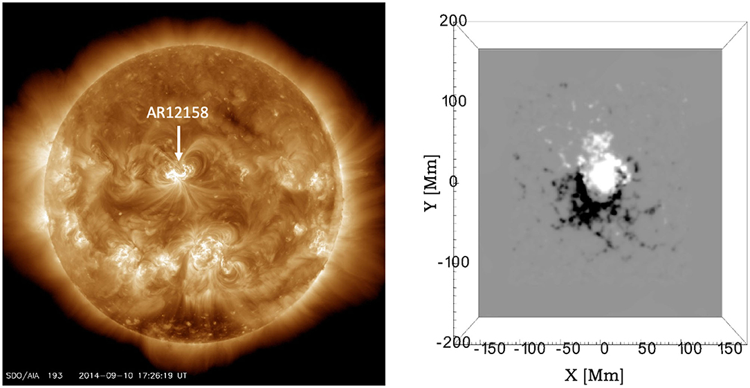
Figure 1. (Left) Extreme Ultraviolet images at 193 Å (Left) taken by SDO/AIA on September 10 2014, 17:10 UT at the early phase of the eruption. The AR12158 is bounded by a white box and it shows the eruptive structure. (Right) Simulation domain shown for the approximately same time. In the Z-direction the domain extends to 150 Mm. The magnetic field in the magnetogram is saturated to ±300 Gauss.

FIGURE 2

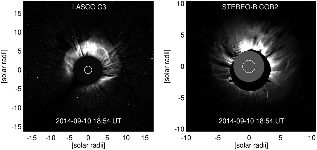
Figure 2. CME morphology as observed by LASCO C3 (left) and STEREO COR2 (right).

A few days later a clear interplanetary CME was detected in the near-Earth solar wind. Figure 3 shows the leading shock on September 12, 15:17 UT as an abrupt jump in the magnetic field magnitude and plasma parameters. The shock is followed by a turbulent sheath and an ejecta. The ejecta showed classical magnetic cloud signatures indicative of a flux rope configuration, i.e., enhanced magnetic field magnitude (Figure 3A), smooth rotation of the field direction (Figure 3B) and depressed plasma beta (Figure 3E). The figure also shows several general ICME signatures (e.g., Zurbuchen and Richardson, 2006; Kilpua et al., 2017a, and references therein) including low magnetic field variability, declining speed profile from front to trailing edge, enhanced oxygen charge ratio O⁺⁷/O⁺⁶ and average iron charge ratio 〈Q_Fe〉 (Figure 3F) as well as bi-directional suprathermal electrons (Figure 3G) during the ejecta. The leading edge of the ejecta occurred on September 12, 21:25 UT and the trailing edge on September 14, 01:45 UT. This end time is selected to coincide at the point where the declining speed ends, plasma beta increases and compositional signatures start to cease. This end time also matches the end time reported in the Richardson and Cane ICME list (http://www.srl.caltech.edu/ACE/ASC/DATA/level3/icmetable2.htm, Richardson and Cane, 2010).

FIGURE 3

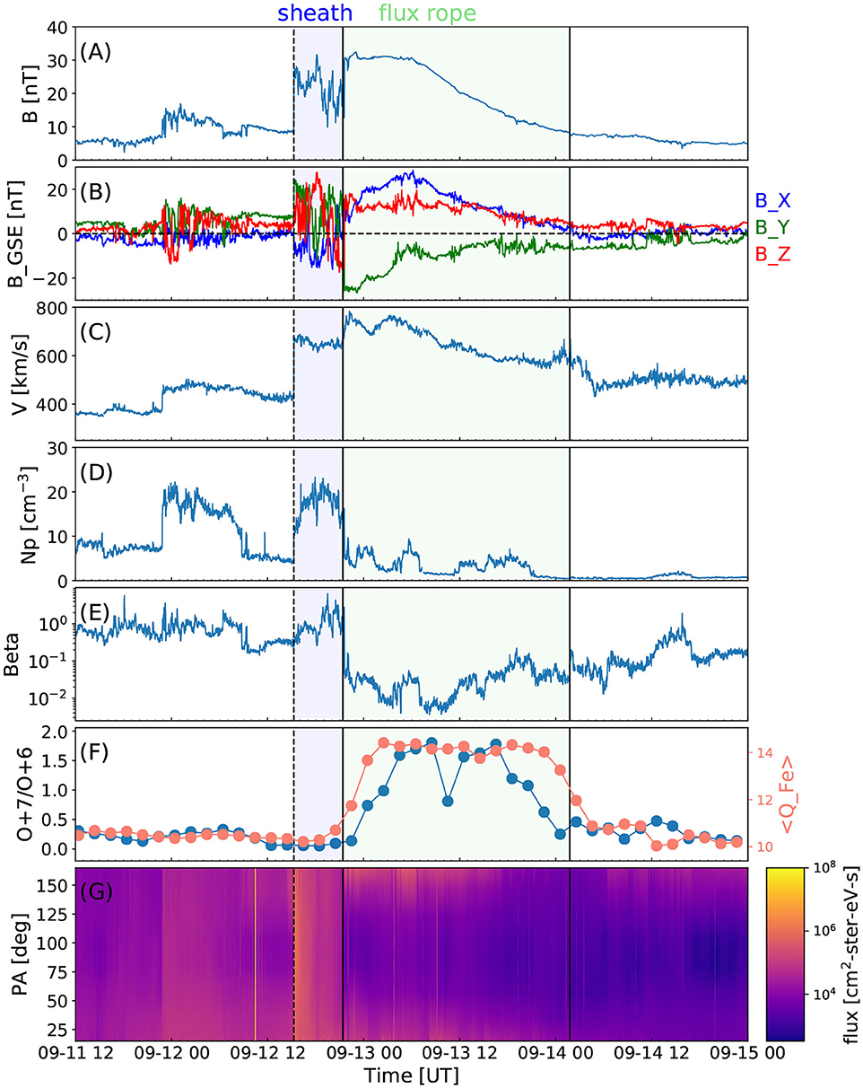
Figure 3. The solar wind in-situ measurements recorded at the Earth's Lagrangian point L1. The panels show, from top to bottom: (A) magnetic field magnitude, (B) magnetic field components in GSE coordinates (blue: B_x, green: B_y, red: B_z), (C) speed, (D) density, (E) plasma beta, (F) oxygen charge state ratio and the average iron charge state, and (G) pitch angle spectrogram of suprathermal 255 eV electrons. The magnetic field and plasma data are from the Wind spacecraft with 1-min resolution, while the 2-h charge state data are from the ACE spacecraft. The suprathermal electron measurements are from Wind. The vertical line marks the shock. The sheath is indicated by the green shaded region and FR by purple-shaded region.

The in situ observations in Figure 3 suggest that the shock of the ICME discussed above intercepted a weak previous ICME. This previous ICME drove a shock, observed on September 11, at 22:49 UT, but the ejecta signatures are not clear, suggesting that Wind made only a glancing encounter. The weak ICME is likely associated with an eruption that occurred early on Sep 9, 2014 from the same AR 12158 with the first appearance in the LASCO field of view at 00:06 UT. The September 9 CME was also a full halo and had a linear speed of 920 km/s. The signatures of the preceding CME are however much weaker and also as indicated by the Space Weather Database Of Notifications, Knowledge, Information (DONKI; https://kauai.ccmc.gsfc.nasa.gov/DONKI/) run (data not shown) the Earth intercepted the September 9, 2014 CME only through its very western and southern flanks. The September 10 CME was in turn encountered clearly more centrally, however also toward its southern part consistent with the coronagraph observations suggesting the propagation north from the ecliptic plane. We therefore conclude that the flux rope in the strong ICME did not have a significant interference from the earlier ICME.

4. Simulation and Flux Rope Identification/Parameters

4.1. Simulation Setup

The magnetogram data, used as input to the electric field inversion, is most reliable when the active region is not too close to the limb. AR 12158 was fully visible from the eastern solar limb by September 5 noon and it was leaving the visible disk (but still fully seen) on September 16 noon. The period when the AR was within ~ 50° from the disk center extends from September 7, ~ 0 UT to September 14, ~ 0 UT. We selected to perform the electric field inversion for this temporal window. The spatial region selected for the inversion is shown in Figure 1. Note that we opted to not apply a masking to the magnetic field data since it yielded the smallest flux imbalance in the dataset (see Supplementary Figure 1).

The temporal evolution of the photospheric energy and helicity injections as provided by the inversion result are shown in Supplementary Figures 2, 3. The electric fields shown in the figures were inverted using the optimal value of U (70 m/s, pink dashed line) and twice the optimal value of U (140 m/s, blue solid line). The reference value from DAVE4VM is shown as the black curve. There is a very good agreement with the optimized U curve and the DAVE4VM curve in terms of the energy injection during the whole simulation, but the helicity injection is overestimated, in particular toward the end of the simulation. Our previous works indicate that helicity injection needs to typically be greatly overestimated to obtain the eruption in the simulation, and thus optimized U typically gives too little helicity to produce the flux rope, see discussion, e.g., in Pomoell et al. (2019).

The simulation was conducted for the twice of the value of optimized U since it yielded the clearest flux rope that ejected from the simulation domain. In our previous studies also (e.g., Price et al., 2020) we have obtained a clear flux rope with the U-assumption.

4.2. Flux Rope Identification

To identify the portion of the domain in the simulation that consists of the flux rope we assume that it consist of highly twisted magnetic field lines that are rooted in the photosphere. The twist value T_w is a measure of the number of turns that the two infinitesimally close magnetic field lines make about each other and it is defined as $T_w=\frac{1}{4\pi }\int ds\frac{{\mu }_0{J}_{\parallel }}{B}$ (see e.g., Berger and Prior, 2006; Liu et al., 2016, and references therein). In this definition J_∥ is the electric current density parallel to the magnetic field and ds is the increment of the arc length along the field line. We define the flux rope to consist of the field lines that have |T_w| > 1 with a constant sign within a coherent region (similar to e.g., Liu et al., 2016; Duan et al., 2019).

In our simulation a coherent structure of negative T_w was seen to form in the lower part of the simulation domain on September 9, around 8 UT that then grows in size when the time progresses. The coherent T_w < −1 structure starts to rise early on September 11 and reaches the upper part of the domain early September 13. The structure also expands as it rises. The snapshots from the twist map and T_w contours in the YZ-plane (placed at X = 0) of the simulation are shown in Figure 4 taken in steps of 24 h. See also the full movie from Supplementary Material. The movie and snapshots show that higher T_w regions (T_w < −1.5 and T_w < −2 contours) form already when the flux rope is still close to the bottom of the simulation domain. These higher T_w region expand with the expanding and rising flux rope, but there is no general drastic increase in T_w.

FIGURE 4

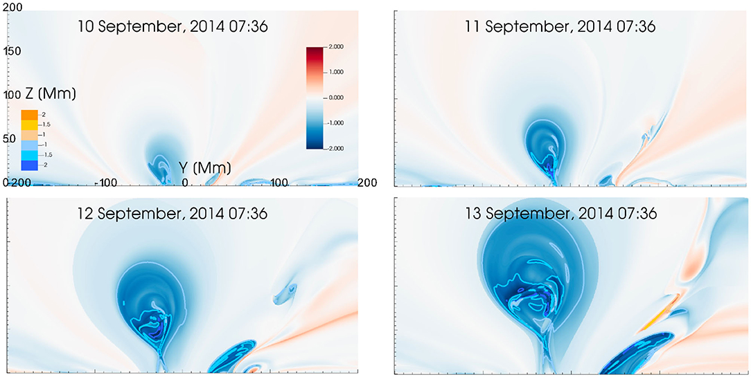
Figure 4. Snapshots of twist number (T_w) maps and T_w countours from the TMFM simulation in steps of 24 h. The colorbar on left shows the contour value with blue colors depicting negative twist contours and orange colors positive twist contours. T_w is a measure of how many turns two field lines that are infinitesimally close make about each other. The colorbar on right shows the T_w map values (blue colors indicate negative T_w, red positive, saturated at ±2).

Figure 5 shows three snapshots from the simulation in the steps of 24 h. In the upper panels the vertical plane of the twist value map and contours are shown in the background while these have been removed in the bottom panels. The field lines that pass through the T_w < −1 contours are drawn and they clearly form a twisted flux rope.

FIGURE 5

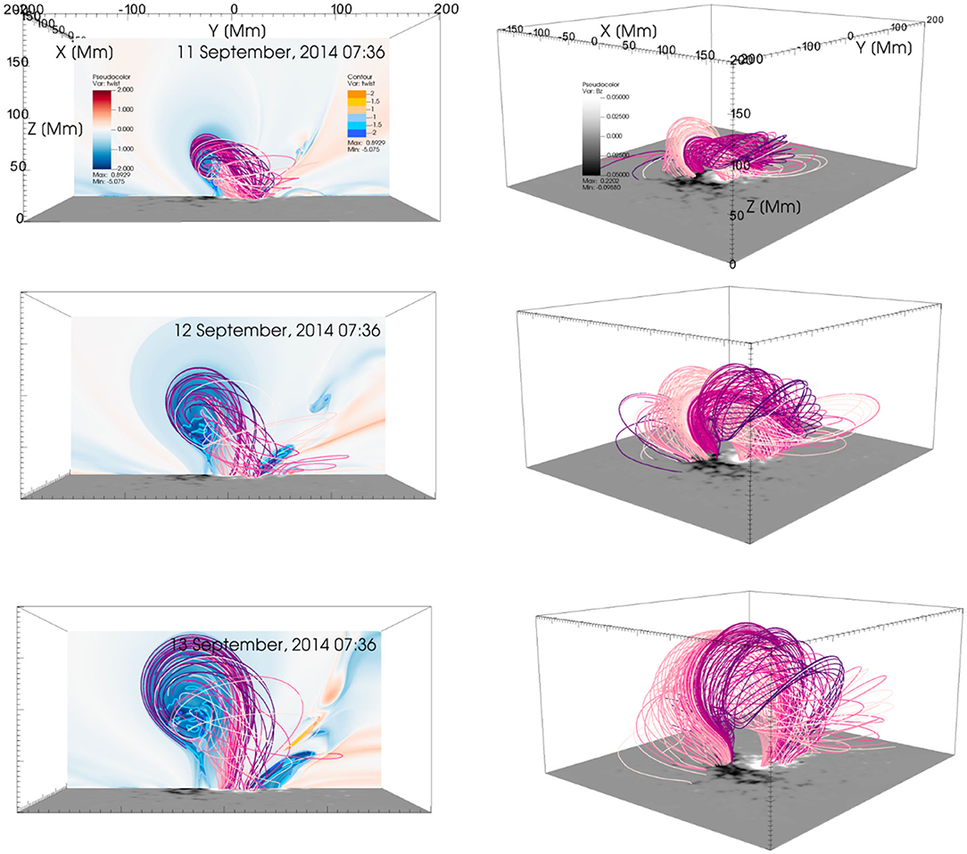
Figure 5. Snapshots from the simulation from 07:36 UT on 11 September, 2014 to 07:36 UT on 13 September with a cadence of 24 h between each snapshot. The top panels show the flux rope field lines where Tw < −1 (different colors depicting different field lines). The flux rope is intercepted with a Tw plane that also shows the contours of Tw. The top panels show the flux rope from a different angle without a slice of Tw and contours. The lower boundary is shown by the B_z on the bottom surface in all plots. The colorbars are same as in Figure 3.

In Figure 6, a set of field lines identified by the above method are drawn and visualized in a view from the top (Right) together with SDO/AIA 131 Å (Middle) EUV images. The time selected is September 10, at 17:10 UT, i.e., when the CME took place at the Sun and the flux rope was still residing close to the bottom of the simulation domain. Here the field lines going through the highest |T_w| core (T_w < −1.5) very close to the bottom of the simulation domain are shown with pink and those above which cross within the T_w < −1.0 contour (but T_w > −1.5) are shown with green (different hues of pink and green represent different individual field lines). Both sets of field lines are traced starting from the strong magnetic field region of positive polarity, but they connect to negative polarities in slightly different regions. The higher lying green lines end to the stronger negative polarity region, while the lower lying pink field lines end to a bit weaker negative field region a bit further away.

FIGURE 6

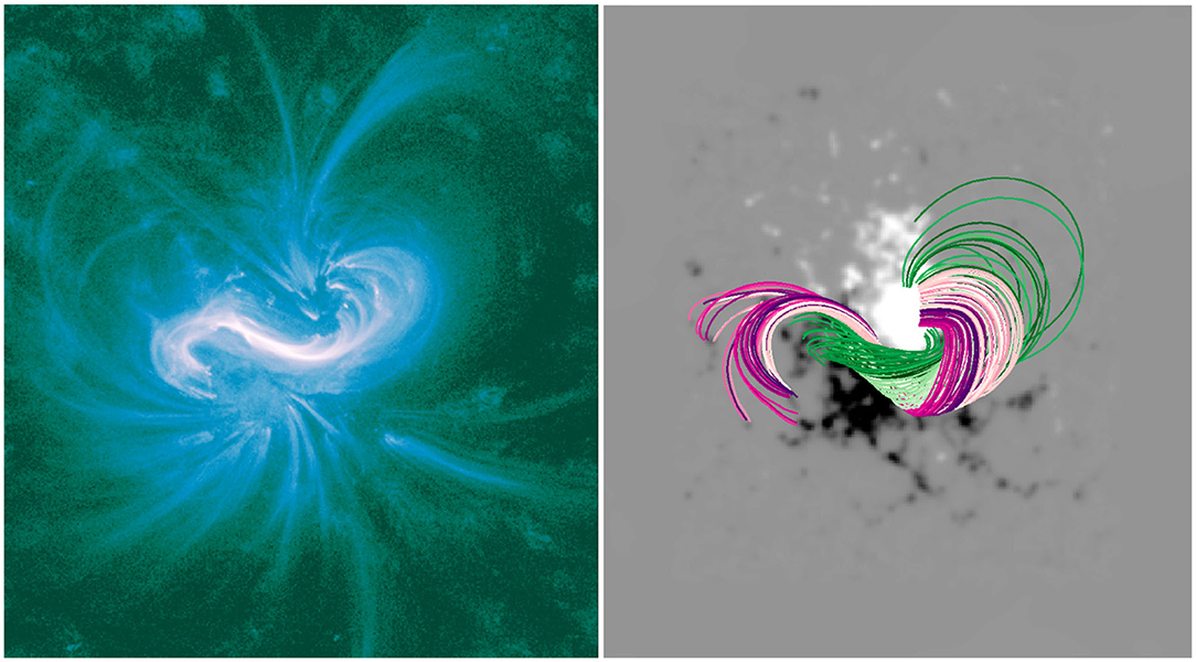
Figure 6. The left panels shows the Extreme Ultraviolet image at 131 Å wavelength taken by SDO/AIA on September 10 2014, 17:10 UT at the early phase of the eruption showing a clear reversed S-shaped sigmoid. The right panel shows a snapshot from the TMFM simulation featuring flux rope field lines with almost at matching time at 17:36 UT. The pink field lines are those intercepting the highest twist T_w < −1.5 contour and green field lines those that intercept the −1.5 < T_w < −1 contour. The magnetic field is saturated to ±300 Gauss.

The flux rope field lines from TMFM simulation match visually well with EUV observations in Figure 6. Both feature a clear inverse S-shaped sigmoid that is considered as a proxy of a flux rope with a negative sign of magnetic helicity (e.g., Rust and Kumar, 1996; Green and Kliem, 2009; Palmerio et al., 2017). The negative helicity sign is also consistent with the “hemispheric rule” (Bothmer and Schwenn, 1998; Pevtsov and Balasubramaniam, 2003) suggesting that magnetic structures on the Sun, including flux ropes, in the northern hemisphere should have a preference for negative helicity, while in the southern hemisphere the dominant helicity is positive. We also note that close to the apex of the TMFM flux rope structure, the field lines run predominantly in a direction that is approximately parallel to the photospheric polarity inversion line.

In the following analysis we will focus on the time when the flux rope had risen close to the top of the simulation domain on September 13, 07:36 UT. This time corresponds to the last times shown in Figures 4, 5 showing the twist value map and twist contours. The flux rope has higher T_w inner part and lower T_w outer part in absolute sense.

4.3. Flux Rope Axis and Apex

For deriving the axial flux and magnetic field cuts through the flux rope the key features that are needed to be identified from the simulation data are the axis of the flux rope and its apex.

The axis of the flux rope is defined using the following scheme: Firstly, for the selected time, we computed the twist value T_w for all closed field lines that passed through the plane close to the photosphere, here the plane Z = R_⊙ + 20 Mm was used, and that had a twist number T_w ≤ −1. Then one of the footpoints of the flux rope was selected, e.g., let's assume that it is the positive polarity foot-point, and all points for which the radial magnetic field component B_r < 0 were removed from the twist map. The resulting map therefore consists of a set of points locating the highly-twisted field lines associated with the positive-polarity foot-point of the flux rope. According to Liu et al. (2016) the spatial variations of T_w can be used to locate the flux rope axis. The authors show that the axis is found as the local extremum, either peak, or a dip, in the T_w map (see also Duan et al., 2019, for example this approach). This method gives thus the coordinates for the axis in the selected plane and those can be used as the seed to draw the axis. For this case, the axis was found as the local minimum. The determination of the axis using T_w, as discussed in Liu et al. (2016), is not straightforward and not a suitable approach for all cases. In this case a local extremum was identified and we note that field lines clearly appear to wind about the common axis found by this method (see Figures 5, 9).

The apex of the flux rope is defined here as the point on the axis with the largest Z value. On September 13, 07:36 UT the apex is located at (X, Y, Z) = (14.3, −41.8, 137.0) Mm.

4.4. Axial Magnetic Flux

In the simulation the axial flux (or toroidal) within the flux rope is computed as ${\varphi }_T={\int }_A\mathbf{\text{B}}·d\mathbf{\text{A}}$, where A is the area of integration in a plane normal to the flux rope axis. Note that the extent of the flux rope is determined to the flux rope identification scheme described in section 4.2.

The results are shown in Table 1. The values are calculated for three different increments in steps of 30 Mm along the axis to the both sides of the apex. Table 1 shows that the fluxes determined from the TMFM flux rope vary between 3.8 × 10²¹–4.1 × 10²¹ Mx and are thus very consistent to within 4%. Since magnetic flux should be constant through the flux rope this gives further support that the axis and extent of the flux rope are robustly determined. We also checked the axial flux at two earlier times on September 12 at and September 11 at 07:36 UT. The values are 4.0 × 10²¹ and 3.6 × 10²¹ Mx.

TABLE 1

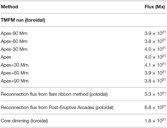
Table 1. Magnetic flux in the flux rope as determined from the TMFM method and from different observational methods (see text for details).

5. Comparison to Observations

In this section we compare the axial magnetic fluxes in the flux rope identified from the performed TMFM simulation (section 4.4) with the magnetic fluxes estimated using different observational methods as well as defined lineouts through the flux rope to investigate how much they vary with distance from the apex and compare the result to in-situ observations.

5.1. Comparison of Axial Magnetic Flux to Observational Proxies

We estimate both the axial and poloidal fluxes in the flux rope using various observational methods that were briefly described in the Introduction. Firstly, we estimate the reconnection flux using both the post-eruptive arcades (PEA) and flare ribbon methods (See the Introduction). These methods give the reconnection flux that can be interpreted as the poloidal flux added to the flux rope via magnetic reconnection during its eruption (see the Introduction). The panels (A) and (B) in Figure 7 illustrate the flare ribbons as seen in AIA 1,600 Å image and the radial component of HMI magnetogram with cumulative flare ribbon area overlying the positive and negative magnetic field polarities depicted with the red and blue regions, respectively. The panels (C) and (D) show the PEA and the HMI magnetogram where the PEA area is delimited with a dashed red box. In order to select the end boundaries of the elongated area underlying the post-eruption arcades, we have followed the extent of the flare ribbons so that we can get rid of the projection effect that may arise due to the presence of post-eruption loops at the end boundaries. The PEAs were very well-formed in this case and their inclination follows roughly that of the EUV sigmoid and PIL, and thus the axis of the TMFM flux rope. Table 1 shows that both flare ribbon and PEA methods give poloidal fluxes of similar orders of magnitude, ≈ 6 × 10²¹ Mx.

FIGURE 7

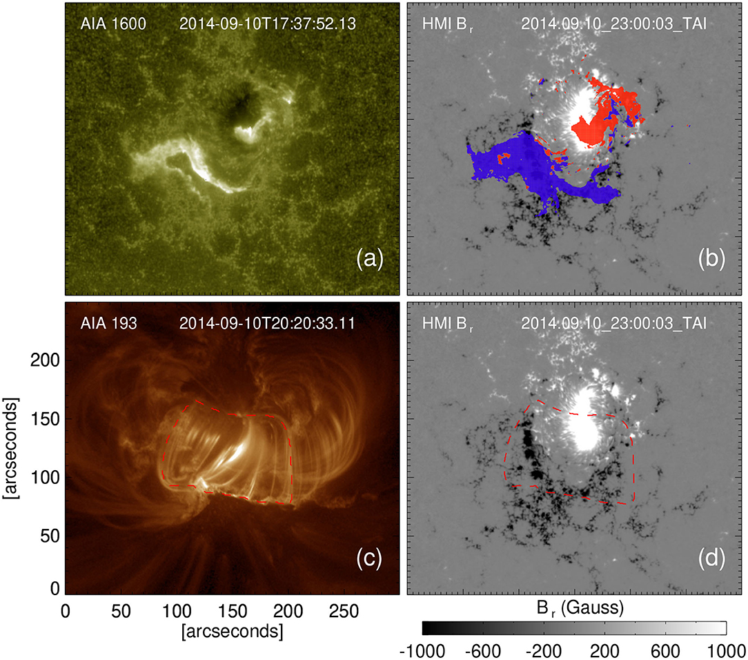
Figure 7. (a) Depicts the flare ribbon in AIA 1,600 Å image. The red dashed boundary line in (c) marks the post-eruption arcades (PEAs) in AIA 193 Å image. (b,d) Illustrate the radial component of HMI vector magnetic field. The red and blue regions in (b) depict the cumulative flare ribbon area overlying the positive and negative magnetic field, respectively. The red dashed boundary in (d) is the over-plotted PEA region.

In order to estimate the toroidal flux of the flux rope, we identified the core dimming region using the method given by Dissauer et al. (2018a). The left and middle panels of Figure 8 show the minimum intensity maps obtained from AIA 211Å images for the logarithmic base ratio and base difference images, and the right panels co-spatial line-of-sight magnetogram with red contours showing the area of core dimming. Computing half of the total unsigned magnetic flux underlying the core dimming regions we obtained the toroidal flux as ≈ 2 × 10²¹ Mx. We noticed that the identification of core dimming regions in our analysis may include projection effects due to the large erupting structure associated with the CME eruption and therefore, may not give the true estimation of the toroidal flux. The estimation of toroidal flux from core dimming method indicates that the magnitude of toroidal flux inside the flux rope is lower than the content of poloidal flux as estimated from the flare ribbon and PEA methods.

FIGURE 8

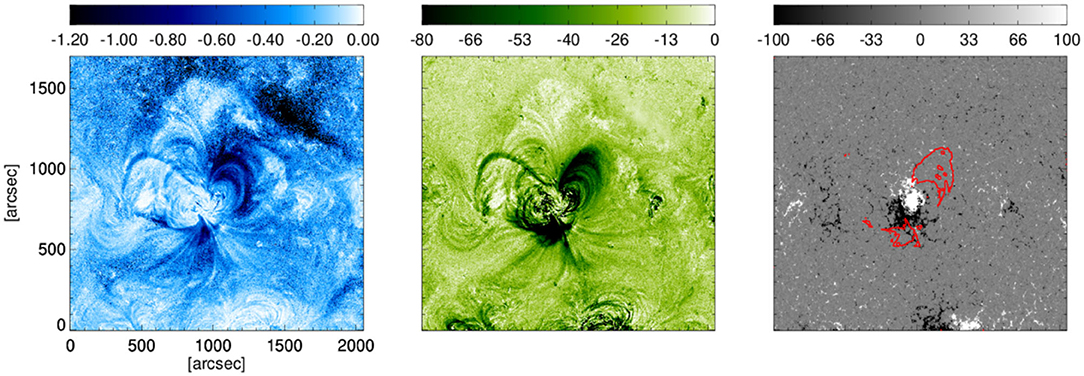
Figure 8. Left panel shows the minimum intensity map of logarithmic base ratio images obtained from the sequence of AIA 211 Angstrom images. Middle panel shows the minimum intensity map of base difference images obtained from the sequence of AIA 211 Angstrom images. Right panel shows the co spatial line-of-sight magnetogram. The red contours denote the core dimming area.

5.2. Magnetic Field Lineouts and Comparison to in-situ Observations

To obtain a prediction of the magnetic field time series at Earth from the simulation we define lineouts through the TMFM flux rope. The lineouts are made through the apex of the flux rope and through different distances from the apex along the flux rope axis. In Figure 9 we show the flux rope axis as a black thick curve and the cut through the apex is denoted by a black vertical line. The selected distances from the apex are three steps to both directions with 30 Mm increments along the axis. These are indicated in the figure with blue (subtracted from the apex point) and red (added to the apex point) vertical lines.

FIGURE 9

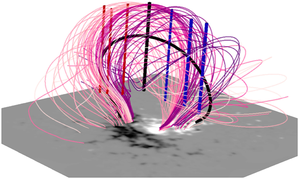
Figure 9. Lineouts through the flux rope through the apex (black vertical line), and different distances from the apex along the axis (blue and red vertical lines) in steps of 30 Mm. The axis of the flux rope is shown with a thick black curve. Field lines are shown with different colors.

The TMFM magnetic field time series are obtained through these lineouts and are then transformed to correspond to the GSE coordinates with a simple transformation. If we assume that the flux rope propagates directly from Sun to Earth the TMFM Z-direction corresponds to the GSE −x direction, TMFM X-direction to the GSE −y direction, and finally TMFM Y-direction to the GSE z direction.

In order to compare the temporal profiles of the magnetic field magnitude and field components from the TMFM to in-situ observations we need to scale the TMFM magnetic field time-series. There are two effects to consider. Firstly, the magnetic field magnitude in the simulation domain and within the flux rope decreases considerably from the bottom to the upper part of the domain. This is featured in Figure 10 showing the magnetic field magnitude in the TMFM YZ-plane centered at X = 14.2 Mm and the negative twist contours for September 13, 07:36 UT. When the flux rope rises higher up in the corona and propagates in interplanetary space it is expected to relax to have a more uniform magnetic field magnitude within. In addition, we need to consider the general decrease of the magnetic field in the heliosphere from the Sun to the Earth. Since we are here just visually comparing the general trends in the magnetic field profiles between the TMFM flux rope and the in-situ magnetic cloud data, we simply use a constant scaling factor for all points that gives a rough match for this case between the magnetic field magnitudes. This means that we do not capture the possible front to rear asymmetries related to the expansion of the ICME flux ropes. To compensate for these two effects we apply a scaling of $(1/s){(Z_0/Z)}^2$ in the TMFM flux rope magnetic field time-series, where s = 100 and where Z₀ is the height at the bottom part of the flux rope. The choice of s = 100 was based on obtaining the approximate match between the magnetic field magnitudes from TMFM simulation and in-situ observations to account for interplanetary field decrease. For more realistic forecasting the change in the magnetic field magnitude could be achieved e.g., by using TMFM results to constrain flux ropes in semi-empirical flux rope models or first principle simulations.

FIGURE 10

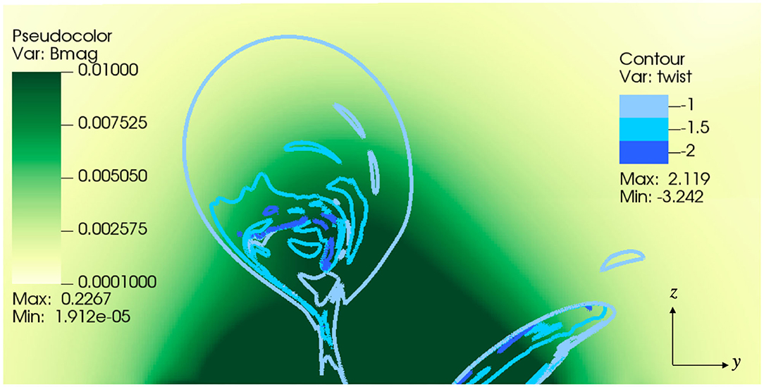
Figure 10. TMFM magnetic field magnitude map of the YZ-plane centered at X = 14.2 Mm and the negative high twist contours on September 13, 07:36 UT in the simulation.

The results of the direct comparison are shown in Figure 11 giving from top to bottom the magnetic field magnitude and GSE magnetic field x, y, and z components. The gray lines show the values measured at 1 AU, while the black, red and blue curves show different cuts through the TMFM flux rope transformed to GSE coordinates as described above. In the magnetic cloud observed by Wind B_x rotates quickly from ~0 at the flux rope leading edge to its maximum value (~ 20 nT) and then rotates slowly back to zero at the trailing edge. B_y rotates from its peak negative value (~ − 20 nT) during the beginning of the cloud to around 0 nT for the trailing portion, while the B_z is positive and rotates from peak value of ~ 20 nT close to zero.

FIGURE 11

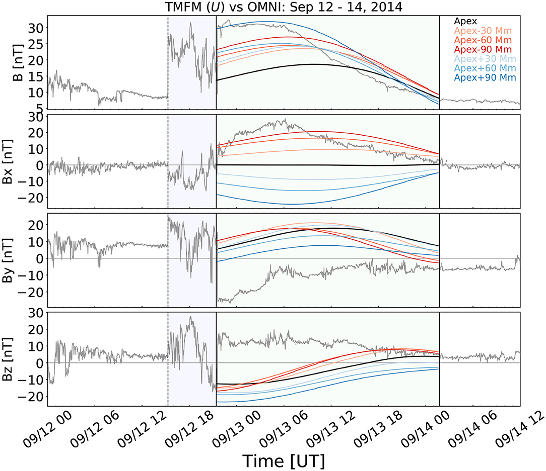
Figure 11. Direct comparison of the TMFM results on September 12, 2014 at 12:36 UT to in-situ observations in the Near-Earth solar wind for seven different cuts along the axis of the flux rope. The black line is the cut through the apex of the flux rope (x = 14 Mm, y = −42 Mm). The blue (red) curves are when 30, 60, and 90 Mm distance along the axis are added to (subtracted from) the apex.

Firstly, we note that the helicity sign of the magnetic cloud is negative as reported also in the Wind ICME list (https://wind.nasa.gov/ICMEindex.php, Nieves-Chinchilla et al., 2018) based on the circular-cylindrical flux rope analytical model (Nieves-Chinchilla et al., 2016). The helicity sign thus corresponds to the helicity sign of the simulated TMFM flux rope as well as that of the EUV sigmoids.

Figure 11 shows that the scaling in the lower corona [${(Z_0/Z)}^2$] yields sensible magnetic field profiles. For example, the magnetic field magnitude in the cut taken through the apex (the black line) peaks approximately close to the axis of the flux rope (remember that we did not consider here expansion in interplanetary space). In addition, the figure shows that the simulation produces flux rope like rotations in all three components. The agreement with the in-situ observations is however not very good. None of the lineouts capture the positive GSE B_z in the flux rope. Only the red curves have positive B_z in the trailing part of the flux rope. The negative B_y in the beginning of the in-situ flux rope is also not captured, while the red curves show positive B_x similar to in-situ flux rope. We also tried several additional lineouts (data not shown) that were made at different distances in the y-direction from the axis at different distances along it. None of these showed a significantly improved match with the in-situ observations.

Differences between the TMFM estimates and in-situ observations can be due to evolution and deformation of the CME flux rope after it left the lower corona and/or due geometrical reasons, i.e., if the observing spacecraft crossed the flux rope loop significantly from below or above. The angle between the shock normal and the radial direction for this event is 29°, indicating the crossing from the intermediate distance from the apex of the flux rope (for the method see e.g., Janvier et al., 2015; Savani et al., 2015). The flux rope reconstruction in the Wind magnetic cloud list gives a very large impact factor of y₀/R = −0.925 (where y₀ is the closest approach distance of the spacecraft from the flux rope axis and R the flux rope radius) and the axis orientation with longitude ϕ = 350° and latitude ϕ = 9°. The quality of the reconstruction is not good for this case, but the above features clearly indicate that this magnetic cloud was not centrally encountered at Earth.

The TMFM B_Y maps (corresponding roughly the expected GSE B_Z in interplanetary space) in the XY plane for three different heights in the corona from close to the apex of the flux rope (Z = 150 Mm, left panel) to mid/bottom part of the flux rope (Z = 70 Mm, right panel) are shown in Figure 12. This figure shows that no matter how the lineouts are made through the flux rope, we do not get negative GSE B_Z in the front part of the flux rope. It could be that the Earth and the spacecraft at L1 intercepted only the lower part of the flux rope. This is consistent with coronagraph observations and DONKI ENLIL runs showing that the CME in question propagated northward of the ecliptic.

FIGURE 12

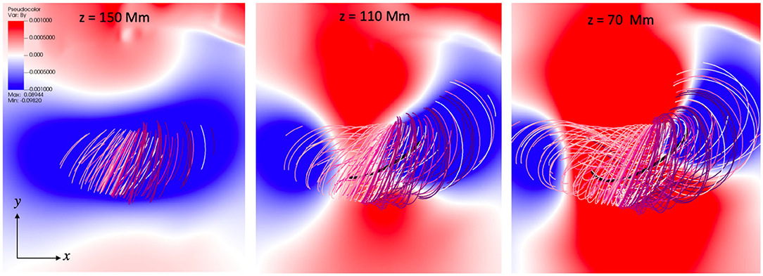
Figure 12. TMFM flux rope field lines and the magnetic field B_y maps (corresponding roughly the GSE B_Z) in the xy-plane at three different heights in the corona.

Another important point clearly visible from Figure 11 is the sensitivity of the magnetic field profiles extracted from the TMFM flux rope to the point where the cut is made. For this case this is particularly clear for the field magnitude and for the GSE B_x component. For the B_y and B_z the variations are less drastic, but still up to about ~ 10 nT difference in the magnitude. For the cuts made away from the axis differences are even larger.

6. Summary and Discussion

In this paper we have performed a fully data-driven simulation of the eruptive solar flux rope that formed into a CME observed on September 10, 2014 that originated from active region 12158. The data-driven simulation is based on the time-dependent magnetofrictional method (TMFM) that uses the electric field inverted from a time-series of photospheric vector magnetograms as its sole boundary condition. We described here the method to extract the flux rope from the simulation data based on the twist number (T_w) maps and extracting its key parameters.

Our simulation produced a very well-defined flux rope that rose through the simulation domain. The flux rope was identified as a coherent region of increased twist number (|T_w| > 1) according to the definition in Liu et al. (2016), in this case the twist was negative. Regions of higher |T_w| formed during the early flux rope formation, but we did not find significant increase in |T_w| as the flux rope rose.

The non-inductive electric field component of the photospheric boundary condition has been found critical for producing the flux rope and its eruption (section 2.2). We constrained it here using the ad-hoc assumption. It is an important and interesting question how the non-inductive electric field should be energy-optimized, in particular for the space weather purposes that requires a quick approach. Based on the studies conducted so far it seems that TMFM needs typically an overestimation of the helicity injection compared to the DAVE4VM reference value. The optimization is also done for the whole active region, while it is typically only a part of it that is involved in the eruption. Constraining of electric fields in TMFM can be done also using different approaches, e.g., using the PDFI (Poloidal-toroidal-decomposition-Doppler-Fourier-local-correlation-tracking-Ideal) electric field inversion method (Kazachenko et al., 2014). Using the preset range of ad-hoc U and Ω values in TMFM could however be a viable and quick solution for space weather forecasting purposes as they require only magnetograms as the input. Such approach however requires that the flux rope parameters (when it is produced in the simulation) do not change significantly depending on the U or Ω value. It is indeed hinted in our previous studies (Pomoell et al., 2019) that one cannot discriminate between the runs based only on energy injection.

The axis of the flux rope was determined using the state-of-the-art method in Liu et al. (2016) that is based on finding the local extremum in twist number T_w. For our case the extremum (minimum) could be located and the field lines visually wound about the common axis. We however note that the determination of the flux rope axis using this approach might not always be this straightforward (e.g., multiple local extremum due to complex twist distribution). Investigating the flux rope axis determination techniques and their robustness from the simulation data is needed.

We found a very good visual agreement between the TMFM simulated flux rope field lines and the EUV observations of a sigmoidal structure at the time of the CME eruption. Both the simulation and observations also indicated that the flux rope had negative magnetic helicity. The obtained results are in addition in agreement with the previously reported NLFFF extrapolation results of the same event (Vemareddy et al., 2016; Zhao et al., 2016) that also yielded a good correspondence with observations.

Further support for the applicability of TMFM to model solar eruptions was given by the estimation of the axial magnetic flux enclosed by the TMFM flux rope. The obtained axial magnetic flux values remained consistent when calculated at different points along the axis and they matched with the factor of two with the axial flux estimated from the core dimming method. The poloidal fluxes estimated using PEA and flare ribbon techniques, both of which give the estimate of the flux added by magnetic reconnection during the eruption, were higher than the axial flux from the core dimming method and from the simulation, but still the same order of magnitude. The lower estimate for the toroidal flux from the dimming method than the estimate for the poloidal flux from the flare ribbon method found in this study is in agreement with the result obtained from the statistical study by Sindhuja and Gopalswamy (2020). Some studies have however also indicated a significant increase in toroidal flux due to flare reconnection during the CME eruption (e.g., Xing et al., 2020). The temporal evolution of axial/poloidal fluxes and twist in flux ropes, and determination of those from the simulation data, are complicated research questions that require more extensive future investigations.

The extracted magnetic field lineouts through different parts of the TMFM flux rope are useful for giving the first estimate of the space weather response, although we emphasize that significant evolution and deformations can take place during the coronal and interplanetary propagation and interactions (e.g., Manchester et al., 2017). We also performed a scaling of the magnetic field to account for the magnetic field gradient in the lower corona in the simulation domain and the general decrease of the field in interplanetary space (see section 5.2).

For the investigated event the direct comparison of the TMFM derived time series of the magnetic field components (transferred straightforwardly to GSE coordinates) with in-situ observations did not produce a good visual agreement with any of the lineouts we made through the TMFM flux rope. The mismatch between the in-situ observations and TMFM predictions in this case is likely due to the Earth intercepting primarily the lower part of the CME, i.e., missing largely the southward fields in the top part of the flux rope. This is consistent with the CME propagating northward from the ecliptic as seen from the coronagraph imagery (section 3). As stated above, the discrepancy between the magnetic field time series estimated directly using the flux rope in the low corona and in-situ ones are also expected to arise due to deflections, rotation, expansion and deformations the CME flux rope may experience between the Sun and the Earth. The magnetic field time-series in the near-Earth solar wind associated with the September 10 CME were also estimated in a parametric study by An et al. (2019) using a 3D heliospheric MHD simulation Reproduce Plasma Universe (REPPU) with a spheromak CME model injected at 38 solar radii. The results showed that the magnetic field time series from the simulation varied significantly depending on the parameters of the injected CMEs, highlighting the importance of having the knowledge of realistic input values to magnetized CME models.

Our study also revealed that the resulting magnetic field magnitude and component profiles are very sensitive to how the lineout was made through the TMFM flux rope. This further emphasizes the importance to accurately forecast how the flux rope intercepts the Earth. In this effort the lower coronal evolution is critical. Several studies have indicated that the most dramatic changes in the propagation direction and tilt of CME flux ropes occurs soon after their eruption, i.e., within a first few solar radii from the Sun (e.g., Kay et al., 2013, 2017; Isavnin et al., 2014).

The simulation run produced the flux rope in the bottom of the simulation at the time corresponding closely to the actual eruption on September 10, 2014. The rise of the flux rope through the simulation domain is however significantly slower than in reality, taking ~2 days. The slow rise is an intrinsic feature of the TMFM method where velocity does not include plasma dynamics terms, but is by the Lorentz force only, see also discussion in Pomoell et al. (2019). This is clearly an issue for long-lead time space weather forecasting. Price et al. (2020) performed relaxation runs to explore the eruption mechanism for the CME flux rope that erupted from the Sun on December 28, 2015 at about 11:30 UT. When the driving was stopped on December 28 at 12 UT, i.e., very shortly after the observed eruption, the rising continued but at a considerably slower rate. When the driving was stopped on December 29 at 12 UT the rise of the flux rope was largely unchanged compared to the case when driving was not stopped (see Figure 8 in Price et al., 2020). That is, the flux rope rise was not due to the photospheric evolution, but consistent with a torus-instability scenario. This means that the “freezing of magnetograms” in TMFM could be applied for space weather forecasting purposes. Another option is that if flux rope parameters do not generally change significantly during the rise, they could be extracted early in the simulation.

To summarize, data-driven and time-dependent modeling of eruptive coronal magnetic fields is a promising method for operational space weather forecasting purposes as they can produce the magnetic structure of CME flux ropes using magnetograms as its sole boundary condition. Time-dependent magnetofrictional method (TMFM) presents a particularly viable option since it is comparatively computationally efficient. This study and previous works (see the Introduction) have clearly demonstrated that TMFM is capable of producing the formation and early evolution of solar flux ropes. We demonstrated here that the intrinsic flux rope parameters can be straightforwardly derived from the TMFM simulation data (such as a twist map, helicity sign, axial magnetic flux and magnetic field lineouts). They are important for giving the early estimate of the space weather response, but the strongest potential of data-driven flux rope modeling approaches in the low corona is expected to come from using them to constrain flux ropes in semi-empirical and first principle models. The success of the predictions from these models is crucially dependent on realistic input values. As discussed in the Introduction the lack of knowledge of the magnetic field properties in CMEs is in particular one of biggest current challenges in space weather predictions. There are however some challenges to be explored further whether the TMFM technique can be adapted as standard forecasting procedure.

Data Availability Statement

The original contributions presented in the study are included in the article/Supplementary Material, further inquiries can be directed to the corresponding author/s. OMNI data was achieved through CDAWeb (https://cdaweb.gsfc.nasa.gov/; Last access: March 11, 2021).

Author Contributions

EK has been the key responsible for writing this paper, compiled the simulation runs, flux rope analysis, and related the figures. JP was the author of the TMFM code and the programs to identify the flux rope and calculating its parameters from the simulation data and assisted in using them. DP has contributed to the writing of optimization programs and assisted in the simulation and analysis process. RS produced the magnetic flux calculations based on observational proxies and produced related figure. EA has made the event identification and assisted in related interpretations. All authors have contributed to the writing of the manuscript and the interpretation of the results.

Funding

This manuscript has received funding from the SolMAG project (ERC-COG 724391) funded by the European Research Council (ERC) in the framework of the Horizon 2020 Research and Innovation Programme, and the Academy of Finland project SMASH 1310445. The results presented in here have been achieved under the framework of the Finnish Centre of Excellence in Research of Sustainable Space (Academy of Finland grant number 312390), which we gratefully acknowledge. We acknowledge H2020 EUHFORIA 2.0 project (870405). EA acknowledges support from the Academy of Finland (Postdoctoral ResearcherGrant 322455).

Conflict of Interest

The authors declare that the research was conducted in the absence of any commercial or financial relationships that could be construed as a potential conflict of interest.

Acknowledgments

We acknowledge A. Szabo for the Wind/MFI data, and K. Ogilvie for the Wind/SWE data. The LASCO CME catalog was generated and maintained at the CDAW Data Center by NASA and The Catholic University of America in cooperation with the Naval Research Laboratory. SOHO was a project of international cooperation between ESA and NASA. SDO data were courtesy of NASA/SDO and the AIA and HMI science teams.

Supplementary Material

The Supplementary Material for this article can be found online at: https://www.frontiersin.org/articles/10.3389/fspas.2021.631582/full#supplementary-material

References

An, J., Magara, T., Hayashi, K., and Moon, Y. J. (2019). Parametric study of ICME properties related to space weather disturbances via a series of three-dimensional MHD simulations. Sol. Phys. 294:143. doi: 10.1007/s11207-019-1531-6

CrossRef Full Text | Google Scholar

Berger, M. A., and Prior, C. (2006). The writhe of open and closed curves. J. Phys. A Math. Gen. 39, 8321–8348. doi: 10.1088/0305-4470/39/26/005

CrossRef Full Text | Google Scholar

Bothmer, V., and Schwenn, R. (1998). The structure and origin of magnetic clouds in the solar wind. Ann. Geophys. 16, 1–24. doi: 10.1007/s00585-997-0001-x

CrossRef Full Text | Google Scholar

Bourdin, P. A. (2017). Plasma beta stratification in the solar atmosphere: a possible explanation for the penumbra formation. Astrophys. J. Lett. 850:L29. doi: 10.3847/2041-8213/aa9988

CrossRef Full Text | Google Scholar

Brueckner, G. E., Howard, R. A., Koomen, M. J., Korendyke, C. M., Michels, D. J., Moses, J. D., et al. (1995). The large angle spectroscopic coronagraph (LASCO). Sol. Phys. 162, 357–402. doi: 10.1007/BF00733434

CrossRef Full Text | Google Scholar

Burlaga, L., Sittler, E., Mariani, F., and Schwenn, R. (1981). Magnetic loop behind an interplanetary shock: Voyager, Helios, and IMP 8 observations. J. Geophys. Res. 86, 6673–6684. doi: 10.1029/JA086iA08p06673

CrossRef Full Text | Google Scholar

Cane, H. V., Richardson, I. G., and Wibberenz, G. (1997). Helios 1 and 2 observations of particle decreases, ejecta, and magnetic clouds. J. Geophys. Res. 102, 7075–7086. doi: 10.1029/97JA00149

CrossRef Full Text | Google Scholar

Chen, J. (2017). Physics of erupting solar flux ropes: coronal mass ejections (CMEs), recent advances in theory and observation. Phys. Plasmas 24:090501. doi: 10.1063/1.4993929

CrossRef Full Text | Google Scholar

Cheung, M. C. M., De Pontieu, B., Tarbell, T. D., Fu, Y., Tian, H., Testa, P., et al. (2015). Homologous helical jets: observations by IRIS, SDO, and Hinode and magnetic modeling with data-driven simulations. Astrophys. J. 801:83. doi: 10.1088/0004-637X/801/2/83

CrossRef Full Text | Google Scholar

Cheung, M. C. M., and DeRosa, M. L. (2012). A method for data-driven simulations of evolving solar active regions. Astrophys. J. 757:147. doi: 10.1088/0004-637X/757/2/147

CrossRef Full Text | Google Scholar

Dissauer, K., Veronig, A. M., Temmer, M., Podladchikova, T., and Vanninathan, K. (2018a). On the detection of coronal dimmings and the extraction of their characteristic properties. Astrophys. J. 855:137. doi: 10.3847/1538-4357/aaadb5

CrossRef Full Text | Google Scholar

Dissauer, K., Veronig, A. M., Temmer, M., Podladchikova, T., and Vanninathan, K. (2018b). Statistics of coronal dimmings associated with coronal mass ejections. I. Characteristic dimming properties and flare association. Astrophys. J. 863:169. doi: 10.3847/1538-4357/aad3c6

CrossRef Full Text | Google Scholar

Domingo, V., Fleck, B., and Poland, A. I. (1995). The SOHO mission: an overview. Sol. Phys. 162, 1–37. doi: 10.1007/BF00733425

CrossRef Full Text | Google Scholar

Duan, A., Jiang, C., He, W., Feng, X., Zou, P., and Cui, J. (2019). A study of pre-flare solar coronal magnetic fields: magnetic flux ropes. Astrophys. J. 884:73. doi: 10.3847/1538-4357/ab3e33

CrossRef Full Text | Google Scholar

Duan, A., Jiang, C., Hu, Q., Zhang, H., Gary, G. A., Wu, S. T., et al. (2017). Comparison of two coronal magnetic field models to reconstruct a sigmoidal solar active region with coronal loops. Astrophys. J. 842:119. doi: 10.3847/1538-4357/aa76e1

CrossRef Full Text | Google Scholar

Dungey, J. W. (1961). Interplanetary magnetic field and the auroral zones. Phys. Rev. Lett. 6, 47–48. doi: 10.1103/PhysRevLett.6.47

CrossRef Full Text | Google Scholar

Fisher, G. H., Abbett, W. P., Bercik, D. J., Kazachenko, M. D., Lynch, B. J., Welsch, B. T., et al. (2015). The coronal global evolutionary model: using HMI vector magnetogram and Doppler data to model the buildup of free magnetic energy in the solar corona. Space Weather 13, 369–373. doi: 10.1002/2015SW001191

CrossRef Full Text | Google Scholar

Gary, G. A. (2001). Plasma beta above a solar active region: rethinking the paradigm. Sol. Phys. 203, 71–86. doi: 10.1023/A:1012722021820

CrossRef Full Text | Google Scholar

Gloeckler, G., Cain, J., Ipavich, F. M., Tums, E. O., Bedini, P., Fisk, L. A., et al. (1998). Investigation of the composition of solar and interstellar matter using solar wind and pickup ion measurements with SWICS and SWIMS on the ACE spacecraft. Space Sci. Rev. 86, 497–539. doi: 10.1023/A:1005036131689

CrossRef Full Text | Google Scholar

Gonzalez, W. D., Joselyn, J. A., Kamide, Y., Kroehl, H. W., Rostoker, G., Tsurutani, B. T., et al. (1994). What is a geomagnetic storm? J. Geophys. Res. 99, 5771–5792. doi: 10.1029/93JA02867

CrossRef Full Text | Google Scholar

Gopalswamy, N., Akiyama, S., Yashiro, S., and Xie, H. (2018). “A new technique to provide realistic input to CME forecasting models,” in Space Weather of the Heliosphere: Processes and Forecasts, Volume 335 of IAU Symposium, eds C. Foullon and O. E. Malandraki, 258–262. doi: 10.1017/S1743921317011048

CrossRef Full Text | Google Scholar

Gopalswamy, N., Yashiro, S., Akiyama, S., and Xie, H. (2017). Estimation of reconnection flux using post-eruption arcades and its relevance to magnetic clouds at 1 AU. Sol. Phys. 292:65. doi: 10.1007/s11207-017-1080-9

CrossRef Full Text | Google Scholar

Green, L. M., and Kliem, B. (2009). Flux rope formation preceding coronal mass ejection onset. Astrophys. J. Lett. 700, L83–L87. doi: 10.1088/0004-637X/700/2/L83

CrossRef Full Text | Google Scholar

Green, L. M., Török, T., Vršnak, B., Manchester, W., and Veronig, A. (2018). The origin, early evolution and predictability of solar eruptions. Space Sci. Rev. 214:46. doi: 10.1007/s11214-017-0462-5

CrossRef Full Text | Google Scholar

Howard, R. A., Moses, J. D., Vourlidas, A., Newmark, J. S., Socker, D. G., Plunkett, S. P., et al. (2008). Sun earth connection coronal and heliospheric investigation (SECCHI). Space Sci. Rev. 136, 67–115. doi: 10.1007/s11214-008-9341-4

CrossRef Full Text | Google Scholar

Huttunen, K. E. J., Schwenn, R., Bothmer, V., and Koskinen, H. E. J. (2005). Properties and geoeffectiveness of magnetic clouds in the rising, maximum and early declining phases of solar cycle 23. Ann. Geophys. 23, 625–641. doi: 10.5194/angeo-23-625-2005

CrossRef Full Text | Google Scholar

Isavnin, A., Vourlidas, A., and Kilpua, E. K. J. (2014). Three-dimensional evolution of flux-rope CMEs and its relation to the local orientation of the heliospheric current sheet. Sol. Phys. 289, 2141–2156. doi: 10.1007/s11207-013-0468-4

CrossRef Full Text | Google Scholar

James, A. W., Valori, G., Green, L. M., Liu, Y., Cheung, M. C. M., Guo, Y., et al. (2018). An observationally constrained model of a flux rope that formed in the solar corona. Astrophys. J. Lett. 855:L16. doi: 10.3847/2041-8213/aab15d

CrossRef Full Text | Google Scholar

Janvier, M., Dasso, S., Démoulin, P., Masías-Meza, J. J., and Lugaz, N. (2015). Comparing generic models for interplanetary shocks and magnetic clouds axis configurations at 1 AU. J. Geophys. Res. 120, 3328–3349. doi: 10.1002/2014JA020836

CrossRef Full Text | Google Scholar

Jian, L., Russell, C. T., Luhmann, J. G., and Skoug, R. M. (2006). Properties of interplanetary coronal mass ejections at one AU during 1995–2004. Sol. Phys. 239, 393–436. doi: 10.1007/s11207-006-0133-2

CrossRef Full Text | Google Scholar

Jiang, C., Wu, S. T., Feng, X., and Hu, Q. (2016). Data-driven magnetohydrodynamic modelling of a flux-emerging active region leading to solar eruption. Nat. Commun. 7:11522. doi: 10.1038/ncomms11522

PubMed Abstract | CrossRef Full Text

Kaiser, M. L., Kucera, T. A., Davila, J. M., St. Cyr, O. C., Guhathakurta, M., and Christian, E. (2008). The STEREO mission: an introduction. Space Sci. Rev. 136, 5–16. doi: 10.1007/s11214-007-9277-0

CrossRef Full Text | Google Scholar

Kay, C., Gopalswamy, N., Reinard, A., and Opher, M. (2017). Predicting the magnetic field of earth-impacting CMEs. Astrophys. J. 835:117. doi: 10.3847/1538-4357/835/2/117

CrossRef Full Text | Google Scholar

Kay, C., Opher, M., and Evans, R. M. (2013). Forecasting a coronal mass ejection's altered trajectory: ForeCAT. Astrophys. J. 775:5. doi: 10.1088/0004-637X/775/1/5

CrossRef Full Text | Google Scholar

Kazachenko, M. D., Fisher, G. H., and Welsch, B. T. (2014). A comprehensive method of estimating electric fields from vector magnetic field and Doppler measurements. Astrophys. J. 795:17. doi: 10.1088/0004-637X/795/1/17

CrossRef Full Text | Google Scholar

Kazachenko, M. D., Lynch, B. J., Welsch, B. T., and Sun, X. (2017). A database of flare ribbon properties from the solar dynamics observatory. I. Reconnection flux. Astrophys. J. 845:49. doi: 10.3847/1538-4357/aa7ed6

CrossRef Full Text | Google Scholar

Kilpua, E., Koskinen, H. E. J., and Pulkkinen, T. I. (2017a). Coronal mass ejections and their sheath regions in interplanetary space. Liv. Rev. Sol. Phys. 14:5. doi: 10.1007/s41116-017-0009-6

PubMed Abstract | CrossRef Full Text | Google Scholar

Kilpua, E. K. J., Balogh, A., von Steiger, R., and Liu, Y. D. (2017b). Geoeffective properties of solar transients and stream interaction regions. Space Sci. Rev. 212, 1271–1314. doi: 10.1007/s11214-017-0411-3

CrossRef Full Text | Google Scholar

Kilpua, E. K. J., Jian, L. K., Li, Y., Luhmann, J. G., and Russell, C. T. (2011). Multipoint ICME encounters: pre-STEREO and STEREO observations. J. Atmos. Sol. Terrest. Phys. 73, 1228–1241. doi: 10.1016/j.jastp.2010.10.012

CrossRef Full Text | Google Scholar

Kilpua, E. K. J., Lugaz, N., Mays, M. L., and Temmer, M. (2019). Forecasting the structure and orientation of earthbound coronal mass ejections. Space Weather 17, 498–526. doi: 10.1029/2018SW001944

CrossRef Full Text | Google Scholar

Klein, L. W., and Burlaga, L. F. (1982). Interplanetary magnetic clouds at 1 AU. J. Geophys. Res. 87, 613–624. doi: 10.1029/JA087iA02p00613

CrossRef Full Text | Google Scholar

Lemen, J. R., Title, A. M., Akin, D. J., Boerner, P. F., Chou, C., Drake, J. F., et al. (2012). The atmospheric imaging assembly (AIA) on the solar dynamics observatory (SDO). Sol. Phys. 275, 17–40. doi: 10.1007/s11207-011-9776-8

CrossRef Full Text | Google Scholar

Lepping, R. P., Acũna, M. H., Burlaga, L. F., Farrell, W. M., Slavin, J. A., Schatten, K. H., et al. (1995). The wind magnetic field investigation. Space Sci. Rev. 71, 207–229. doi: 10.1007/BF00751330

CrossRef Full Text | Google Scholar

Lin, R. P., Anderson, K. A., Ashford, S., Carlson, C., Curtis, D., Ergun, R., et al. (1995). A three-dimensional plasma and energetic particle investigation for the wind spacecraft. Space Sci. Rev. 71, 125–153. doi: 10.1007/BF00751328

CrossRef Full Text | Google Scholar

Liu, R., Kliem, B., Titov, V. S., Chen, J., Wang, Y., Wang, H., et al. (2016). Structure, stability, and evolution of magnetic flux ropes from the perspective of magnetic twist. Astrophys. J. 818:148. doi: 10.3847/0004-637X/818/2/148

CrossRef Full Text | Google Scholar

Lugaz, N., Farrugia, C. J., Manchester, W. B. IV, and Schwadron, N. (2013). The interaction of two coronal mass ejections: influence of relative orientation. Astrophys. J. 778:20. doi: 10.1088/0004-637X/778/1/20

CrossRef Full Text | Google Scholar

Lumme, E., Pomoell, J., and Kilpua, E. K. J. (2017). Optimization of photospheric electric field estimates for accurate retrieval of total magnetic energy injection. Sol. Phys. 292:191. doi: 10.1007/s11207-017-1214-0

CrossRef Full Text | Google Scholar

Manchester, W., Kilpua, E. K. J., Liu, Y. D., Lugaz, N., Riley, P., Török, T., et al. (2017). The physical processes of CME/ICME evolution. Space Sci. Rev. 212, 1159–1219. doi: 10.1007/s11214-017-0394-0

CrossRef Full Text | Google Scholar

Möstl, C., Amerstorfer, T., Palmerio, E., Isavnin, A., Farrugia, C. J., Lowder, C., et al. (2018). Forward modeling of coronal mass ejection flux ropes in the inner heliosphere with 3DCORE. Space Weather 16, 216–229. doi: 10.1002/2017SW001735

PubMed Abstract | CrossRef Full Text | Google Scholar

Nieves-Chinchilla, T., Linton, M. G., Hidalgo, M. A., Vourlidas, A., Savani, N. P., Szabo, A., et al. (2016). A circular-cylindrical flux-rope analytical model for magnetic clouds. Astrophys. J. 823:27. doi: 10.3847/0004-637X/823/1/27

CrossRef Full Text | Google Scholar

Nieves-Chinchilla, T., Vourlidas, A., Raymond, J. C., Linton, M. G., Al-haddad, N., Savani, N. P., et al. (2018). Understanding the internal magnetic field configurations of ICMEs using more than 20 years of wind observations. Sol. Phys. 293:25. doi: 10.1007/s11207-018-1247-z

CrossRef Full Text | Google Scholar

Odstrcil, D., Riley, P., and Zhao, X. P. (2004). Numerical simulation of the 12 May 1997 interplanetary CME event. J. Geophys. Res. 109:A02116. doi: 10.1029/2003JA010135

CrossRef Full Text | Google Scholar

Ogilvie, K. W., Chornay, D. J., Fritzenreiter, R. J., Hunsaker, F., Keller, J., Lobell, J., et al. (1995). SWE: a comprehensive plasma instrument for the wind spacecraft. Space Sci. Rev. 71, 55–77. doi: 10.1007/BF00751326

CrossRef Full Text | Google Scholar

Ogilvie, K. W., and Desch, M. D. (1997). The wind spacecraft and its early scientific results. Adv. Space Res. 20, 559–568. doi: 10.1016/S0273-1177(97)00439-0

CrossRef Full Text | Google Scholar

Palmerio, E., Kilpua, E. K. J., James, A. W., Green, L. M., Pomoell, J., Isavnin, A., et al. (2017). Determining the intrinsic CME flux rope type using remote-sensing solar disk observations. Sol. Phys. 292:39. doi: 10.1007/s11207-017-1063-x

CrossRef Full Text | Google Scholar

Palmerio, E., Kilpua, E. K. J., Möstl, C., Bothmer, V., James, A. W., Green, L. M., et al. (2018). Coronal magnetic structure of earthbound CMEs and in situ comparison. Space Weather 16, 442–460. doi: 10.1002/2017SW001767

CrossRef Full Text | Google Scholar

Pesnell, W. D., Thompson, B. J., and Chamberlin, P. C. (2012). The solar dynamics observatory (SDO). Sol. Phys. 275, 3–15. doi: 10.1007/s11207-011-9841-3

CrossRef Full Text | Google Scholar

Pevtsov, A. A., and Balasubramaniam, K. S. (2003). Helicity patterns on the sun. Adv. Space Res. 32, 1867–1874. doi: 10.1016/S0273-1177(03)90620-X

CrossRef Full Text | Google Scholar

Pomoell, J., Lumme, E., and Kilpua, E. (2019). Time-dependent data-driven modeling of active region evolution using energy-optimized photospheric electric fields. Sol. Phys. 294:41. doi: 10.1007/s11207-019-1430-x

PubMed Abstract | CrossRef Full Text | Google Scholar

Pomoell, J., and Poedts, S. (2018). EUHFORIA: European heliospheric forecasting information asset. J. Space Weather Space Clim. 8:A35. doi: 10.1051/swsc/2018020

CrossRef Full Text | Google Scholar

Price, D. J., Pomoell, J., and Kilpua, E. K. J. (2020). Exploring the coronal evolution of AR 12473 using time-dependent, data-driven magnetofrictional modelling. Astron. Astrophys. 644:A28. doi: 10.1051/0004-6361/202038925

CrossRef Full Text | Google Scholar

Price, D. J., Pomoell, J., Lumme, E., and Kilpua, E. K. J. (2019). Time-dependent data-driven coronal simulations of AR 12673 from emergence to eruption. Astron. Astrophys. 628:A114. doi: 10.1051/0004-6361/201935535

CrossRef Full Text | Google Scholar

Pulkkinen, T. (2007). Space weather: terrestrial perspective. Liv. Rev. Sol. Phys. 4:1. doi: 10.12942/lrsp-2007-1

CrossRef Full Text | Google Scholar

Richardson, I. G., and Cane, H. V. (2010). Near-earth interplanetary coronal mass ejections during solar cycle 23 (1996–2009): catalog and summary of properties. Sol. Phys. 264, 189–237. doi: 10.1007/s11207-010-9568-6

CrossRef Full Text | Google Scholar

Richardson, I. G., and Cane, H. V. (2012). Solar wind drivers of geomagnetic storms during more than four solar cycles. J. Space Weather Space Clim. 2:A01. doi: 10.1051/swsc/2012001

CrossRef Full Text | Google Scholar

Rust, D. M., and Kumar, A. (1996). Evidence for helically kinked magnetic flux ropes in solar eruptions. Astrophys. J. Lett. 464:L199. doi: 10.1086/310118

CrossRef Full Text | Google Scholar

Sarkar, R., Gopalswamy, N., and Srivastava, N. (2020). An observationally constrained analytical model for predicting the magnetic field vectors of interplanetary coronal mass ejections at 1 au. Astrophys. J. 888:121. doi: 10.3847/1538-4357/ab5fd7

CrossRef Full Text | Google Scholar

Savani, N. P., Vourlidas, A., Szabo, A., Mays, M. L., Richardson, I. G., Thompson, B. J., et al. (2015). Predicting the magnetic vectors within coronal mass ejections arriving at Earth: 1. Initial architecture. Space Weather 13, 374–385. doi: 10.1002/2015SW001171

CrossRef Full Text | Google Scholar

Scherrer, P. H., Schou, J., Bush, R. I., Kosovichev, A. G., Bogart, R. S., Hoeksema, J. T., et al. (2012). The helioseismic and magnetic imager (HMI) investigation for the solar dynamics observatory (SDO). Sol. Phys. 275, 207–227. doi: 10.1007/s11207-011-9834-2

CrossRef Full Text | Google Scholar

Schuck, P. W. (2008). Tracking vector magnetograms with the magnetic induction equation. Astrophys. J. 683, 1134–1152. doi: 10.1086/589434

CrossRef Full Text | Google Scholar

Scolini, C., Chané, E., Temmer, M., Kilpua, E. K. J., Dissauer, K., Veronig, A. M., et al. (2020). CME-CME interactions as sources of CME geoeffectiveness: the formation of the complex ejecta and intense geomagnetic storm in 2017 early September. Astrophys. J. Suppl. 247:21. doi: 10.3847/1538-4365/ab6216

CrossRef Full Text | Google Scholar

Scolini, C., Rodriguez, L., Mierla, M., Pomoell, J., and Poedts, S. (2019). Observation-based modelling of magnetised coronal mass ejections with EUHFORIA. Astron. Astrophys. 626:A122. doi: 10.1051/0004-6361/201935053

CrossRef Full Text | Google Scholar

Shiota, D., and Kataoka, R. (2016). Magnetohydrodynamic simulation of interplanetary propagation of multiple coronal mass ejections with internal magnetic flux rope (SUSANOO-CME). Space Weather 14, 56–75. doi: 10.1002/2015SW001308

CrossRef Full Text | Google Scholar

Sindhuja, G., and Gopalswamy, N. (2020). A study of the observational properties of coronal mass ejection flux ropes near the sun. Astrophys. J. 889:104. doi: 10.3847/1538-4357/ab620f

CrossRef Full Text | Google Scholar

Stone, E. C., Frandsen, A. M., Mewaldt, R. A., Christian, E. R., Margolies, D., Ormes, J. F., et al. (1998). The advanced composition explorer. Space Sci. Rev. 86, 1–22. doi: 10.1023/A:1005082526237

CrossRef Full Text | Google Scholar

Tsurutani, B. T., Lakhina, G. S., and Hajra, R. (2020). The physics of space weather/solar-terrestrial physics (STP): what we know now and what the current and future challenges are. Nonlin. Process. Geophys. 27, 75–119. doi: 10.5194/npg-27-75-2020

CrossRef Full Text | Google Scholar

van Ballegooijen, A. A., Priest, E. R., and Mackay, D. H. (2000). Mean field model for the formation of filament channels on the sun. Astrophys. J. 539, 983–994. doi: 10.1086/309265

CrossRef Full Text | Google Scholar

Vasyliunas, V. M. (1975). Theoretical models of magnetic field line merging. I. Rev. Geophys. 13, 303–336. doi: 10.1029/RG013i001p00303

CrossRef Full Text | Google Scholar

Vemareddy, P., Cheng, X., and Ravindra, B. (2016). Sunspot rotation as a driver of major solar eruptions in the NOAA active region 12158. Astrophys. J. 829:24. doi: 10.3847/0004-637X/829/1/24

CrossRef Full Text | Google Scholar

Verbeke, C., Pomoell, J., and Poedts, S. (2019). The evolution of coronal mass ejections in the inner heliosphere: implementing the spheromak model with EUHFORIA. Astron. Astrophys. 627:A111. doi: 10.1051/0004-6361/201834702

CrossRef Full Text | Google Scholar

Vourlidas, A., Patsourakos, S., and Savani, N. P. (2019). Predicting the geoeffective properties of coronal mass ejections: current status, open issues and path forward. Philos. Trans. A Math. Phys. Eng. Sci. 377:20180096. doi: 10.1098/rsta.2018.0096

PubMed Abstract | CrossRef Full Text | Google Scholar

Webb, D. F., and Howard, T. A. (2012). Coronal mass ejections: observations. Liv. Rev. Sol. Phys. 9:3. doi: 10.12942/lrsp-2012-3

CrossRef Full Text | Google Scholar

Webb, D. F., Lepping, R. P., Burlaga, L. F., DeForest, C. E., Larson, D. E., Martin, S. F., et al. (2000). The origin and development of the May 1997 magnetic cloud. J. Geophys. Res. 105, 27251–27260. doi: 10.1029/2000JA000021

CrossRef Full Text | Google Scholar

Wiegelmann, T., and Sakurai, T. (2012). Solar force-free magnetic fields. Liv. Rev. Sol. Phys. 9:5. doi: 10.12942/lrsp-2012-5

CrossRef Full Text | Google Scholar

Xing, C., Cheng, X., Qiu, J., Hu, Q., Priest, E. R., and Ding, M. D. (2020). Quantifying the toroidal flux of preexisting flux ropes of coronal mass ejections. Astrophys. J. 889:125. doi: 10.3847/1538-4357/ab6321

CrossRef Full Text | Google Scholar

Yang, W. H., Sturrock, P. A., and Antiochos, S. K. (1986). Force-free magnetic fields: the magneto-frictional method. Astrophys. J. 309:383. doi: 10.1086/164610

CrossRef Full Text | Google Scholar

Yardley, S. L., Mackay, D. H., and Green, L. M. (2018). Simulating the coronal evolution of AR 11437 using SDO/HMI magnetograms. Astrophys. J. 852:82. doi: 10.3847/1538-4357/aa9f20

CrossRef Full Text | Google Scholar

Zhang, J., Liemohn, M. W., Kozyra, J. U., Lynch, B. J., and Zurbuchen, T. H. (2004). A statistical study of the geoeffectiveness of magnetic clouds during high solar activity years. J. Geophys. Res. 109:A09101. doi: 10.1029/2004JA010410

CrossRef Full Text | Google Scholar

Zhang, J., Richardson, I. G., Webb, D. F., Gopalswamy, N., Huttunen, E., Kasper, J. C., et al. (2007). Solar and interplanetary sources of major geomagnetic storms (Dst ≤ −100 nT) during 1996–2005. J. Geophys. Res. 112:A10102. doi: 10.1029/2007JA012321

CrossRef Full Text | Google Scholar

Zhao, J., Gilchrist, S. A., Aulanier, G., Schmieder, B., Pariat, E., and Li, H. (2016). Hooked flare ribbons and flux-rope-related QSL footprints. Astrophys. J. 823:62. doi: 10.3847/0004-637X/823/1/62

CrossRef Full Text | Google Scholar

Zurbuchen, T. H., and Richardson, I. G. (2006). In-situ solar wind and magnetic field signatures of interplanetary coronal mass ejections. Space Sci. Rev. 123, 31–43. doi: 10.1007/s11214-006-9010-4

CrossRef Full Text | Google Scholar