Homogeneous vs Biased IGM: Impact on Reionization

1 Introduction

Epoch of Reionization (EoR) is considered as one of the most difficult challenges in modern cosmology (see e.g., Shapiro and Giroux, 1987; Gnedin and Ostriker, 1997; Barkana and Loeb, 2001, Barkana and Loeb, 2005; Furlanetto et al., 2009; Zaroubi, 2013; Cooray et al., 2019). Analysis of the EoR is demanding on observational (see e.g., Tozzi et al., 2000; Bernardi et al., 2009; Harker et al., 2010; Parsons et al., 2010; Hazelton et al., 2013; Thyagarajan et al., 2015; Dillon and Parsons, 2016; Thyagarajan et al., 2016; Mertens et al., 2018; Barry et al., 2019; Greig et al., 2020) as well as theoretical (see e.g., Madau et al., 1997; Ciardi et al., 2000; Benson et al., 2006; Furlanetto et al., 2006; Mesinger et al., 2011; Giri et al., 2018; Qin et al., 2018; La Plante and Ntampaka, 2019; Park et al., 2019; Liu and Shaw, 2020) fronts. The possibility of observing EoR in the radio window using the 21 cm radiation was suggested a long time ago (Wouthuysen, 1952; Field, 1959b; Sunyaev and Zeldovich, 1975). The 21 cm line emitted by the neutral hydrogen in the IGM gets redshifted to much larger wavelengths and a continuous distribution of neutral hydrogen gives rise to a continuum of emission in the radio window (for reviews, see Fan et al., 2006; Furlanetto et al., 2006; Choudhury, 2009; Pritchard and Loeb, 2012).

This paper explores the impact of large scale biasing of the IGM on the 21 cm power spectrum from EoR. Many earlier works have considered a clumpy IGM during the EoR (see e.g., Kohler et al., 2007; Pawlik et al., 2009; McQuinn et al., 2011; Raičević and Theuns, 2011; Finlator et al., 2012; Emberson et al., 2013; Jeeson-Daniel et al., 2014; So et al., 2014; Sobacchi and Mesinger, 2014; Trombetti and Burigana, 2014; Mao et al., 2020). Such an IGM is granular or clustered on small scales and is considered on subgrid level. Its eventual impact on the EoR power spectrum is considered by some authors (see e.g., Mao et al., 2020). This paper addresses large scale clumping or large scale biasing of the IGM. By large scale biasing one means how the distribution of the IGM is in the whole simulation box. Many numerical approaches of simulating EoR assume IGM to be having uniform density far from halo boundaries (see e.g., Mellema et al., 2006; Thomas and Zaroubi, 2008; Thomas et al., 2009; Ghara et al., 2015). While the early versions of semi-analytic methods determine the neutral hydrogen fraction, $x_{HI}$, based on excursion sets arguments and then assume that the hydrogen density follows the dark matter density (see e.g., Choudhury et al., 2009; Mesinger et al., 2011). Now, the hydrogen in the IGM could have a more complicated dependence on the local density of the massive haloes. So the regions of the universe that have more or less massive halos also have more or less density of the background IGM. The simplest way to consider this is through following expression:

${\rho }_H^{IGM}\propto \left(1+\alpha {\delta }_{collapsed massive haloes}\right)(1)$

In this work, α is termed as the IGM bias parameter and it notifies the biasing of the IGM with respect to the collapsed massive haloes¹. For $\alpha =0$, the IGM is uniform which means that the uncollapsed gas is distributed uniformly in the Inter-Galactic regions. For $\alpha =1$, the IGM is biased in the way that its density is proportional to the collapsed matter density: ${\rho }^{IGM}\propto \left(1+{\delta }_{collapsed massive haloes}\right)$. These are the two extremes the models suggested by Eq. 1 take. Note that as $\langle 1+\alpha \cdot \delta \rangle =1$, introduction of alpha does not change the value of mean or global amount of neutral hydrogen. It only changes its distribution. It is seen in this work that the two extreme distributions, given by $\alpha =0$ and $\alpha =1$, could have very different power spectra. As 21 cm power spectrum is one the prime observables of the EoR, this work suggests that the distribution of the IGM with respect to the collapsed matter should be studied in more depth in order to gain a proper understanding of the epoch.

The paper is organized as follows: The next section discusses the method of generating the 21 cm maps. The method is ideally suited to address the problem of impact of a biased IGM on EoR. The later section discusses the main results of the paper. A prescription for the IGM bias parameter within the Press-Schechter framework is then derived. This is followed by the conclusion of the work in the last section.

2 Method for Generating 21 cm Maps

The method used in this work (Raut, 2019) borrows ideas of semi-analytic methods (Furlanetto et al., 2004; Choudhury et al., 2009; Mesinger et al., 2011) and extensively numerical methods (Razoumov and Scott, 1999; Abel et al., 1999; Nakamoto et al., 2001). The parameters that are borrowed from semi-analytic approach are: $M_{\min }$ (minimum mass of collapsed haloes), $n_{ion}$ (number of ionizing photons deposited in the IGM per collapsed baryon in stars) and $n_{rec}$ (number representing the ratio of ionization rate to recombination rate). This method has similarities with the hybrid approaches of Trac and Cen (2007); Lee et al. (2008); Zheng et al. (2011), but it is computationally less demanding as it emphasizes upon the scales of interests ($0.1Mp{c}^{-1}\mathrm{\lesssim }k\mathrm{\lesssim }1.0Mp{c}^{-1}$). Upcoming radio telescopes like HERA (DeBoer et al., 2017)² and SKA1-Low (Koopmans et al., 2015)³ will be more sensitive to these modes (Kulkarni et al., 2016). The fiducial values of reionization parameters used in this work are: $M_{\min }={10}^8{M}_{\odot }$, $n_{rec}=1$ and ${\overline{x}}_{HI}=\left\{0.4,0.6,0.75\right\}$ for $z=\left\{\mathrm{7,8,9}\right\}$ (denotes the mean or global value of neutral hydrogen fraction.) The details of the method used for generating 21 cm maps is ${\overline{x}}_{HI}$ as follows:

• The first step is to do N-body simulations and compute overdensity for each grid cell. I have used Illustris-1 simulations (Genel et al., 2014) for this step. The cosmological parameters used are wmap-9 (Hinshaw et al., 2013): ${\Omega }_M=0.2726$, ${\Omega }_b=0.0456$, ${\sigma }_8=0.821$ and $h=0.704$. The box-size is $106.5Mpc$ and gridsize is ${64}^3$. This paper uses a method that is a small modification to the one used in the earlier work. Instead of using excursions sets (Press and Schechter, 1974; Bardeen et al., 1986; Bond et al., 1991; Lacey and Cole, 1993)to find out the collapsed fraction $f_{coll}$, one uses the total halo distribution itself to find the extent of collapsed structure. The $M_{\min }$ provided by above n-body simulations is about ${10}^8{M}_{\odot }$ and so this approach is justified.

Second step assigns ionizing photons to each grid cell based on following prescription (Furlanetto et al., 2004).

$\begin{array}{l}{n}_{ion}=f_{esc}\cdot f_{\ast }\cdot N_{\gamma /b}\\ n_{\gamma }\propto n_{ion}\cdot f_{coll}\end{array}$

• Here, $f_{esc}$ is the escape fraction of the ionizing photons, $f_{\ast }$ is the star formation efficiency and $N_{\gamma /b}$ is the number of ionizing photons produced per baryon in stars. $n_{\gamma }$ is the number of ionizing photons produced in a grid cell which has collapse fraction $f_{coll}$.

• The next step is to split all the photons, $N_{\gamma }={\displaystyle \sum _{cells}{n}_{\gamma }}$, into a large number ($\sim {10}^7$) of photon-rays. Each photon ray carries a weight indicating the amount of photons it carries. Initially most of the photon rays have equal weights. Each photon ray is assigned a random position and direction inside the grid cells. Then each photon ray is propagated in small steps, i.e. 0.05 of grid cell size. Note that the number of photon-rays originating in a grid cell is proportional to $\sim {10}^7$ count of that cell.

• The next step is to implement reionization. At each step of propagation of photon-rays, one computes the total weights of the photon-rays arriving in the grid cells. This total is compared with the amount of neutral hydrogen present in the grid cells. The photon-ray weights and neutral hydrogen counts are decremented at every step accounting for reionization. It is assumed at this step that each photon-ray can ionize amount of neutral hydrogen equal to the photon-ray weight (i.e., 100% ionization efficiency or a very large cross section for ionization reaction).

• The next step implements recombination. After the photon-ray weights and neutral hydrogen content of each grid cell is revised, the number of neutral hydrogen atoms that were ionized in that particular step, $n_1$, is computed. This number is computed for each grid cell separately. Before implementation of the next step of photon-ray propagation, $r\cdot n_1$ number of neutral hydrogen atoms are added back to each grid cell to account for recombinations. Here $r=n_{rec}/\left(1+n_{rec}\right)$ and is the ratio of recombination rate to ionization rate.

• The final step is to terminate the photon-ray propagation and assign brightness temperature to each grid cell. The first part is implemented when the total of photon-ray weights falls below 0.1% of its initial value. For the second part, we use the well-known expression (Wouthuysen, 1952; Field, 1959a; Madau et al., 1997; Furlanetto et al., 2006),

$\delta T_b\approx 27x_{HI}\left(1+\delta \right)\left(1-T_{\gamma }/T_s\right){\left(\frac{1+z}{10}\frac{0.15}{{\Omega }_M{h}^2}\right)}^{\frac{1}{2}}\left(\frac{{\Omega }_b{h}^2}{0.023}\right)(2)$

3 The Biased IGM Analysis

This section discusses the effect of biased IGM on 21 cm brightness temperature distribution. The biasing of the IGM is modelled through Eq. 1 in the next two subsections.

3.1 Modification of the 21 cm Brightness Temperature Distribution With the IGM Bias Parameter

The 21 cm maps are generated for three values of α: 0, 0.5, and 1. As suggested earlier, $\alpha =0$ corresponds to an IGM that is distributed uniformly in the whole simulation box, while, $\alpha =1$ corresponds to an IGM that is distributed proportional to the extent of the collapsed structures. This way of assigning IGM to each grid cell could be over simplified and actual distribution of the IGM could be more complicatedly biased with respect to the collapsed matter (see the next section). Here, value of one is used for the recombination parameter, $n_{rec}$ (Sobacchi and Mesinger, 2014) and value of ${10}^8{M}_{\odot }$ is used for the minimum halo mass $M_{\text{min}}$ (Barkana and Loeb, 2001). The $n_{ion}$ values were chosen in such a way so as to produce global neutral hydrogen fraction of 0.4, 0.6, and 0.75 for redshifts 7, 8, and 9 respectively. This set of values of neutral hydrogen fraction is consistent with the CMBR and LyAlpha data (Kulkarni et al., 2016; Raut and Choudhury, 2018). To get the $n_{ion}$ values for each redshift, we solve the following equation ($Y_{He}$ is the Helium fraction):

${\overline{x}}_{HI}=1-\frac{n_{ion}\langle f_{coll}\rangle }{\left(1+n_{rec}\right)\left(1-\langle f_{coll}\rangle \right)\left(1-\frac{Y_{He}}{2}\right)}(3)$

In this work, the global neutral hydrogen fraction, denoted by ${\overline{x}}_{HI}$, is considered as a parameter instead of $n_{ion}$. Once $n_{rec}$ and $\langle f_{coll}\rangle$ values are fixed, above equation uniquely determines the $n_{ion}$ value for a given ${\overline{x}}_{HI}$.

The reionization data cubes are generated as discussed in the previous section. The 21 cm brightness temperature slices (midway through the simulation box) are shown in Figure 1. This is done for three values of the IGM bias parameter ($\alpha =\mathrm{0,0.5},1$) and for three values of redshift ($z=\mathrm{7,8,9}$).

FIGURE 1

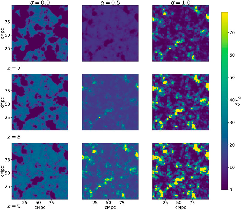
FIGURE 1. Brightness temperature slices midway through the simulation box. The slices are shown for three different values of α for three different redshifts. The values of redshift are indicated at the bottom-left side of each horizontal panel while the α values are shown at the top of each column.

As seen from Figure 1, the topology of the 21 cm brightness temperature distribution is changed as the IGM bias parameter is changed. For $\alpha =0$, it is outside-in with the 21 cm bright regions are surrounding the 21 cm dark regions. While for $\alpha =1$, it is inside-out with the 21 cm bright regions are embedded inside the 21 cm dark regions. This is expected as gas in the voids will remain neutral and hence 21 cm bright for the uniform IGM or $\alpha =0$ case (The hydrogen near collapsed structure will be ionized while the hydrogen away from collapsed structures will remain neutral.) On the other hand, the voids will be devoid of gas and hence 21 cm dark for $\alpha =1$ case. As expected, for the intermediate value of $\alpha =0.5$, the distribution is also intermediate and is close to being uniform.

These conclusions are fortified if one analyzes the 21 cm brightness temperature probability distributions. As seen from Figure 2, the probability distributions are opposite for $\alpha =0$ and $\alpha =1$ case. For $\alpha =0$, there are more bright regions as compared to the dark ones and for $\alpha =1$, there are more dark regions are compared to the bright ones. This is because, voids, which occupy a larger volume, are brighter for $\alpha =0$ case and darker for $\alpha =1$ case. For the intermediate case of $\alpha =0.5$, the plots indicate that the distributions are more or less uniform as they have a single peak and most of the areas in the probability distribution curves are covered by a small range of $\delta T_b$ values.

FIGURE 2

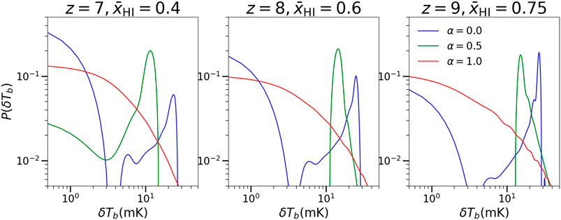
FIGURE 2. The 21 cm brightness temperature probability distribution (smoothed) for the whole simulation box for three values of redshifts and for three values of α The blue line is for the uniform (or for $\alpha =0$) case, the green line is for $\alpha =0.5$ and the red line is for $\alpha =1$ case.

One can also study the impact of the variation of the IGM bias parameter on the power spectrum. To obtain the power spectrum, the standard procedure is followed. First, the 21 cm brightness temperature distribution ($\delta T_b\equiv {\delta }_{21}$) is Fourier transformed and dimensionless power spectrum is obtained using following equations:

$\langle {\tilde{\delta }}_{21}\left(k\right) {\tilde{\delta }}_{21}^{\ast }\left(k^{\prime }\right)\rangle ={\left(2\pi \right)}^3 {\delta }_D\left(k-k^{\prime }\right)P\left(k\right),(4)$

${\Delta }^2\left(k\right)=\frac{k^{3}P\left(k\right)}{2{\pi }^2}.(5)$

The spherically averaged dimensionless power spectrum is the obtained by averaging ${\Delta }^2\left(k\right)$ over all possible angles

${\Delta }^2\left(k\right)=\frac{1}{4\pi }{\displaystyle \underset{-1}{\overset{1}{\int }}d\mu {\displaystyle \underset{0}{\overset{2\pi }{\int }}d\varphi {\Delta }^2\left(k\right)}} (6)$

Here $\mu =k_{\parallel }/k$ is the cosine of the angle that wavevector $k$ makes with the LOS or parallel direction and ϕ is the azimuthal angle.

As seen from Figure 3, for $z=7$, the power spectrum is nearly same for the two extreme scenarios of $\alpha =0$ and $\alpha =1$. One should take note that although the power spectrum is almost the same, the topologies are opposite. For the other two redshifts, though, there is significant enhancement of power for the case of $\alpha =1$. This could be because of combination of larger neutral hydrogen fraction and more isolation of collapsed structures as compared to the $z=7$ case. These two, combined, are producing more contrast in $\delta T_b$ distribution for the $\alpha =1$ case as compared to the $\alpha =0$ case.

FIGURE 3

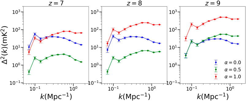
FIGURE 3. The 21 cm brightness temperature distribution power spectrum for three different redshifts for three different values of the IGM bias parameter α. The value of redshift is mentioned at top of each plot while the value of α is mentioned at the bottom right corner of the third plot.

There is also a notable fall in the power spectrum for the $\alpha =0.5$ case for redshifts $z=7$ and $z=8$. As mentioned before, this is because the intermediate value of the IGM bias parameter drives the $\delta T_b$ distribution toward uniformity. This means that distributions of the remnant neutral hydrogen and the collapsed structures are almost perfectly inversely related to each other. Thus the product $x_{HI}\cdot \left(1+{\delta }_b\right)$ that appears in the $\delta T_b$ expression is almost constant. This is giving a nearly constant brightness temperature distribution and very small power spectrum. This behaviour is generic and seems to appear for every redshift for some α (see the discussion in the next subsection).

3.2 The Critical Value of the IGM Bias Parameter and the Uniform Distribution

The severe degradation of the 21 cm brightness temperature power spectrum is one of the main results of this paper and hence some further analysis is justified. Figure 4 shows the dependence of the power for three typical modes for three redshifts as a function of α. As mentioned before, these three modes are representative of the scales that would be measured by upcoming and future experiments. As seen from the figure, behavior of all the modes is similar: the plots are U-shaped. The power goes to almost zero for each mode for some value of α. Notably, this value of α seems to depend on the redshift alone and not on the scales. This means that all the scales hit minima at the same value of α. This observation indicates that there is indeed a near washout of $\delta T_b$ fluctuations in the entire simulation box.

FIGURE 4

FIGURE 4. Dependence of power on the IGM bias parameter, α, for three typical modes for the three redshifts. The value of modes is indicated at the top left corner in the first plot. The value of redshift is indicated at the top of each box.

A critical value of the IGM bias parameter that causes a near uniform brightness temperature distribution is possibly a characteristic of the reionization process. To check this all three reionization parameters are varied from their fiducial values. This is done for the $z=7$ case. As mentioned earlier, the fiducial parameter values are $M_{\min }={10}^8{M}_{\odot }$, $n_{rec}=1$ and ${\overline{x}}_{HI}=0.4$. Figure 5 shows the variation of the three k-modes as a function of the IGM bias parameter for six different combinations of reionization parameters. The central region of the plots indicate the changed parameter while the other two parameters are kept unchanged from their fiducial values. For all the cases, one can see that there is either a critical value of the IGM bias parameter or a range of values of the IGM bias parameter for which there is a low signal. As the signal is nearly zero, this work warrants a careful study of distribution of IGM with respect to the collapsed structures. It should also be noted that the topology of the 21 cm brightness temperature distribution would be opposite on two sides of the critical value of the IGM bias parameter.

FIGURE 5

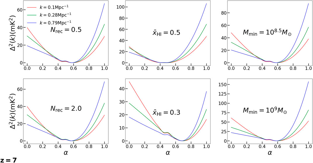
FIGURE 5. Dependence of power on IGM bias parameter, α, for three typical modes for six different variations of reionization parameters. The value of modes is indicated at the top left corner in the first panel. The redshift is indicated at the bottom left. The parameter that is changed is indicated in the central portion of the plots. While one of the reionization parameter is changed, the other two are kept constant.

4 Prescription for IGM Distribution Based on Press-Schechter Theory

The IGM bias parameter being a constant throughout the box is ideally not possible but it is the next step to the other two extreme scenarios of it being equal to one or zero. These two extreme scenarios form basis of the EoR simulations done by many earlier works (see e.g., Mellema et al., 2006; Thomas and Zaroubi, 2008; Choudhury et al., 2009; Thomas et al., 2009; Mesinger et al., 2011; Ghara et al., 2015). A possible next step to a constant value for the IGM bias parameter is an IGM bias parameter that is a function of the overdensity parameter. This could be predicted within the framework of the Press-Schecheter theory. The following assumptions are employed to obtain the IGM distribution within this framework:

• The results of the Press-Schechter theory are exact,

• Baryons follow dark matter,

• All the baryons that are not part of galaxies (i.e., massive collapsed haloes) are considered as being part of the IGM.⁴

Let,

${\delta }_{IGM}\equiv {\delta }_{lmh}\equiv {\delta }_{low mass haloes}(7)$

${\delta }_{cmh}\equiv {\delta }_{collapsed massive haloes}(8)$

It is shown in the Supplementary Appendix that $\alpha ={\delta }_{IGM}/{\delta }_{cmh}$ for a grid cell with overdensity δ and collapse fraction $f_{coll}$ is given by:

$\alpha =\frac{\left(1+\delta \right)\left(1-f_{coll}\right)-\left(1-{\overline{f}}_{coll}\right)}{\left(1+\delta \right)f_{coll}-{\overline{f}}_{coll}}\times \frac{{\overline{f}}_{coll}}{1-{\overline{f}}_{coll}}(9)$

Here ${\overline{f}}_{coll}$ is average or global value of the collapse fraction. Figure 6 shows the dependence of the IGM bias parameter obtained using above equation.

FIGURE 6

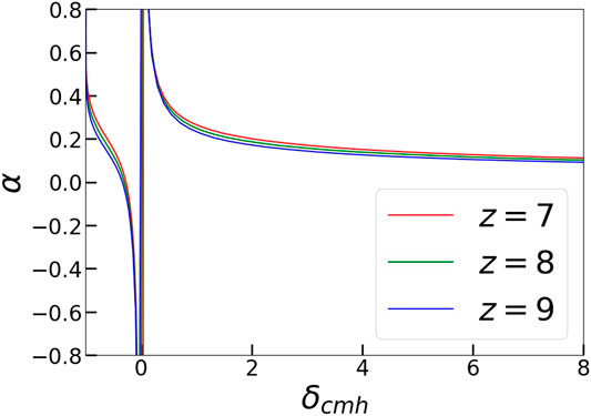
FIGURE 6. Dependence of the IGM bias parameter on the overdensity parameter ${\delta }_{cmh}$ within the Press-Schechter framework.

This prescription should be able to give a good zeroth level baryon distribution. Environmental effects, baryonic physics and other astrophysical effects would give rise to modulations to this distribution. Using this prescription for the IGM density, one can now obtain the 21 cm brightness temperature distribution and it is shown in Figure 7.

FIGURE 7

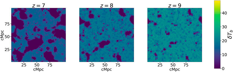
FIGURE 7. Brightness temperature distribution, midway through the simulation box, for the three redshifts obtained using the Press-Schechter prescription.

The under dense grid cells are more in number than the over dense grid cells and they dominate the overall behaviour. For $z=9$, the average value of the IGM bias parameter is about 0.22 and is close to the critical value. As a result, the distribution seen is also nearly uniform. One can find the power spectrum of the 21 cm brightness temperature distribution for the Press-Schechter prescription and compare it to the two extreme scenarios of the uniform and the perfectly biased IGM. The results are shown in Figure 8. As seen from the figure, there is degradation of power for all three cases compared to the other two extreme scenarios. It can also be seen that for $z=9$ there is a severe loss of power for the large scales as the average value of the IGM bias parameter is close to the critical value.

FIGURE 8

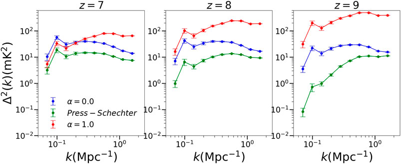
FIGURE 8. Power spectrum of 21 cm brightness temperature distribution for the three redshifts obtained using the Press-Schechter prescription. For comparison, the power spectrum for a uniform IGM and for a perfectly biased IGM is also plotted.

5 Discussion and Conclusion

In this work we discussed how an IGM that is having varied bias with respect to the massive halo population could impact the 21 cm brightness temperature distribution. It is found that the distribution as well as the power spectrum are significantly affected with the difference in the IGM bias parameter α (Eq. 1), while, the global neutral hydrogen fraction remains constant. It is also found that for some critical value of the IGM bias parameter, the distribution becomes almost uniform causing a near washout of the 21 cm power spectrum. This critical value of the IGM bias parameter is different for different redshifts. Thus, it is essential to estimate the large scale distribution of the IGM. In this work, we also saw that this distribution could be estimated within the framework of the Press-Schechter theory. It was also observed that for $z=9$, the framework yielded a nearly uniform distribution. The degradation in the structure of 21 cm brightness temperature distribution occurs because there are more ionizing photons in the regions where there is more neutral hydrogen. This situation can also occur for standard scenarios (i.e. $\alpha =0$ or $\alpha =1$) if one has an $n_{ion}$ that is density dependent. In this work $n_{ion}$ has been assumed to be globally constant. But, consider case of $\alpha =1$ for which neutral hydrogen follows the collapsed matter. If one has larger $n_{ion}$ for over dense regions and smaller $n_{ion}$ for under dense regions then one can arrive at a situation in which the extent of neutral hydrogen in each grid cell is about the same. And so the 21 cm brightness temperature distribution is nearly uniform.

Many early large scale structure studies assume that the baryons follow dark matter or ${\rho }_b\propto {\rho }_{dm}$. It is found in many works that, based on theory (see e.g. Cen and Ostriker, 1999; Springel et al., 2001; He et al., 2005; Zentner et al., 2005; Crain et al., 2007; Diemand et al., 2007; Giocoli et al., 2008; Moster et al., 2018) and observations (see e.g. Fukugita et al., 1998; Ettori, 2003; Dai et al., 2010; McGaugh et al., 2010; Eckert et al., 2016; Chan, 2019), the above assumption need not be valid and more work is needed to get a conclusion on the exact dependence. As suggested by these works, the problem of finding exact dependence of the hydrogen content on the massive collapsed structures is a difficult one. In the realistic scenarios, where baryons do not strictly follow the dark matter, there could be more structure in the 21 cm brightness temperature distribution. This would possibly give more power on small scales. Baryonic physics could alter the bias parameter but the average value over the entire box is likely to remain close to the one obtained using the assumption of baryons following dark matter.

There are possibly two future directions to the problem posed in this work: One could assume that the baryon fraction parameter, $f_b={\Omega }_b/{\Omega }_M$, to be dependent on halo mass and find the its correlation to the halo mass based on observations (see e.g., Padmanabhan et al., 2016) or simulations (see e.g., Genel et al., 2014; Crain et al., 2015; Pillepich et al., 2018; Diemer et al., 2019). One could also take a more direct approach and use the high resolution simulations themselves to use the hydrogen content of various cosmic structures (Martizzi et al., 2019). A very high resolution simulation could directly yield the hydrogen density for the whole simulation box.

The author would like to thank the Illustris collaboration for their N-body simulations. The author would also like to thank anonymous referees whose comments helped in improving the quality of the manuscript.

Both, ${\delta }_{cmh}$ and ${\delta }_{lmh}$, can be obtained as function of true overdensity δ and hence the IGM bias parameter α can be obtained as a function of overdensity of collapsed massive haloes ${\delta }_{cmh}$.

Data Availability Statement

The original contributions presented in the study are included in the article/Supplementary Material, further inquiries can be directed to the corresponding author.

Author Contributions

The author confirms being the sole contributor of this work and has approved it for publication.

Conflict of Interest

The author declares that the research was conducted in the absence of any commercial or financial relationships that could be construed as a potential conflict of interest.

Supplementary Material

The Supplementary Material for this article can be found online at: https://www.frontiersin.org/articles/10.3389/fspas.2021.633007/full#supplementary-material.

Footnotes

¹Note that the bias parameter is defined with respect to collapsed matter density and not with respect to the underlying dark-matter density

²https://reionization.org/

³http://astronomers.skatelescope.org/

⁴The baryons in uncollapsed haloes would give rise to a clumpy IGM. This will modify the recombination parameter and would make it position dependent. This complication is not considered in this work.

References

Abel, T., Norman, M. L., and Madau, P. (1999). Photon-conserving radiative transfer around point sources in multidimensional numerical cosmology. Astrophys. J. 523, 66–71. doi:10.1086/307739

CrossRef Full Text | Google Scholar

Bardeen, J. M., Bond, J. R., Kaiser, N., and Szalay, A. S. (1986). The statistics of peaks of Gaussian random fields. Astrophys. J. 304, 15. doi:10.1086/164143

CrossRef Full Text | Google Scholar

Barkana, R., and Loeb, A. (2005). Detecting the earliest galaxies through two new sources of 21 centimeter fluctuations. Astrophys. J. 626, 1–11. doi:10.1086/429954

CrossRef Full Text | Google Scholar

Barkana, R., and Loeb, A. (2001). In the beginning: the first sources of light and the reionization of the universe. Phys. Rep. 349, 125–238. doi:10.1016/S0370-1573(01)00019-9

CrossRef Full Text | Google Scholar

Barry, N., Wilensky, M., Trott, C. M., Pindor, B., Beardsley, A. P., Hazelton, B. J., et al. (2019). Improving the epoch of reionization power spectrum results from murchison widefield array season 1 observations. Astrophys. J. 884, 16. doi:10.3847/1538-4357/ab40a8

CrossRef Full Text | Google Scholar

Benson, A. J., Sugiyama, N., Nusser, A., and Lacey, C. G. (2006). The epoch of reionization. Mon. Not. R. Astron. Soc. 369, 1055–1080. doi:10.1111/j.1365-2966.2006.10426.x

CrossRef Full Text | Google Scholar

Bernardi, G., de Bruyn, A. G., Brentjens, M. A., Ciardi, B., Harker, G., Jelić, V., et al. (2009). Foregrounds for observations of the cosmological 21 cm line. I. First Westerbork measurements of Galactic emission at 150 MHz in a low latitude field. Astron. Astrophys. 500, 965–979. doi:10.1051/0004-6361/200911627

CrossRef Full Text | Google Scholar

Bond, J. R., Cole, S., Efstathiou, G., and Kaiser, N. (1991). Excursion set mass functions for hierarchical Gaussian fluctuations. Astrophys. J. 379, 440. doi:10.1086/170520

CrossRef Full Text | Google Scholar

Cen, R., and Ostriker, J. P. (1999). Where are the baryons? Astrophys. J. 514, 1–6. doi:10.1086/306949

CrossRef Full Text | Google Scholar

Chan, M. H. (2019). A universal constant for dark matter-baryon interplay. Sci. Rep. 9, 3570. doi:10.1038/s41598-019-39717-x

PubMed Abstract | CrossRef Full Text | Google Scholar

Choudhury, T. R. (2009). Analytical models of the intergalactic medium and reionization. Curr. Sci. 97, 841.

Google Scholar

Choudhury, T. R., Haehnelt, M. G., and Regan, J. (2009). Inside-out or outside-in: the topology of reionization in the photon-starved regime suggested by Lyman-alpha forest data. Mon. Not. R. Astron. Soc. 394, 960–977. doi:10.1111/j.1365-2966.2008.14383.x

CrossRef Full Text | Google Scholar

Ciardi, B., Ferrara, A., Governato, F., and Jenkins, A. (2000). Inhomogeneous reionization of the intergalactic medium regulated by radiative and stellar feedbacks. Mon. Not. R. Astron. Soc. 314, 611–629. doi:10.1046/j.1365-8711.2000.03365.x

CrossRef Full Text | Google Scholar

Cooray, A., Chang, T. C., Unwin, S., Zemcov, M., Coffey, A., Morrissey, P., et al. (2019). Cosmic dawn intensity mapper. Bull. Am. Astron. Soc. 51, 23.

Google Scholar

Crain, R. A., Eke, V. R., Frenk, C. S., Jenkins, A., McCarthy, I. G., Navarro, J. F., et al. (2007). The baryon fraction of 𝜆-CDM haloes. Mon. Not. R. Astron. Soc. 377, 41–49. doi:10.1111/j.1365-2966.2007.11598.x

CrossRef Full Text | Google Scholar

Crain, R. A., Schaye, J., Bower, R. G., Furlong, M., Schaller, M., Theuns, T., et al. (2015). The EAGLE simulations of galaxy formation: calibration of subgrid physics and model variations. Mon. Not. Roy. Astron. Soc. 450, 1937–1961. doi:10.1093/mnras/stv725

CrossRef Full Text | Google Scholar

Dai, X., Bregman, J. N., Kochanek, C. S., and Rasia, E. (2010). On the baryon fractions in clusters and groups of galaxies. Astrophys. J. 719, 119–125. doi:10.1088/0004-637X/719/1/119

CrossRef Full Text | Google Scholar

DeBoer, D. R., Parsons, A. R., Aguirre, J. E., Alexander, P., Ali, Z. S., Beardsley, A. P., et al. (2017). Hydrogen epoch of reionization array (HERA). Pub. Astron. Soc. Pac. 129, 045001. doi:10.1088/1538-3873/129/974/045001

CrossRef Full Text | Google Scholar

Diemand, J., Kuhlen, M., and Madau, P. (2007). Formation and evolution of galaxy dark matter halos and their substructure. Astrophys. J. 667, 859–877. doi:10.1086/520573

CrossRef Full Text | Google Scholar

Diemer, B., Stevens, A. R. H., Lagos, C. d. P., Calette, A. R., Tacchella, S., Hernquist, L., et al. (2019). Atomic and molecular gas in IllustrisTNG galaxies at low redshift. Mon. Not. R. Astron. Soc. 487, 1529–1550. doi:10.1093/mnras/stz1323

CrossRef Full Text | Google Scholar

Dillon, J. S., and Parsons, A. R. (2016). Redundant array configurations for 21 cm cosmology. Astrophys. J. 826, 181. doi:10.3847/0004-637X/826/2/181

CrossRef Full Text | Google Scholar

Eckert, K. D., Kannappan, S. J., Stark, D. V., Moffett, A. J., Berlind, A. A., and Norris, M. A. (2016). Resolve and Eco: the halo mass-dependent shape of galaxy stellar and baryonic mass functions. Astrophys. J. 824, 124. doi:10.3847/0004-637X/824/2/124

CrossRef Full Text | Google Scholar

Emberson, J. D., Thomas, R. M., and Alvarez, M. A. (2013). The opacity of the intergalactic medium during reionization: resolving small-scale structure. Astrophys. J. 763, 146. doi:10.1088/0004-637X/763/2/146

CrossRef Full Text | Google Scholar

Ettori, S. (2003). Are we missing baryons in galaxy clusters? Mon. Not. R. Astron. Soc. 344, L13–L16. doi:10.1046/j.1365-8711.2003.06810.x

CrossRef Full Text | Google Scholar

Fan, X., Carilli, C. L., and Keating, B. (2006). Observational constraints on cosmic reionization. Ann. Rev. Astron. Astrophys. 44, 415–462. doi:10.1146/annurev.astro.44.051905.092514

CrossRef Full Text | Google Scholar

Field, G. B. (1959a). An attempt to observe neutral hydrogen between the galaxies. Astrophys. J. 129, 525. doi:10.1086/146652

CrossRef Full Text | Google Scholar

Field, G. B. (1959b). The spin temperature of intergalactic neutral hydrogen. Astrophys. J. 129, 536. doi:10.1086/146653

CrossRef Full Text | Google Scholar

Finlator, K., Oh, S. P., Özel, F., and Davé, R. (2012). Gas clumping in self-consistent reionization models. Mon. Not. R. Astron. Soc. 427, 2464–2479. doi:10.1111/j.1365-2966.2012.22114.x

CrossRef Full Text | Google Scholar

Fukugita, M., Hogan, C. J., and Peebles, P. J. E. (1998). The cosmic baryon budget. Astrophys. J. 503, 518–530. doi:10.1086/306025

CrossRef Full Text | Google Scholar

Furlanetto, S. R., Lidz, A., Loeb, A., McQuinn, M., Pritchard, J. R., Shapiro, P. R., et al. (2009). “Cosmology from the highly-redshifted 21 cm line,” in Astro2010: the Astronomy and astrophysics decadal survey (The National Academic Press), 2010, 82.

Google Scholar

Furlanetto, S. R., Oh, S. P., and Briggs, F. H. (2006). Cosmology at low frequencies: the 21 cm transition and the high-redshift Universe. Phys. Rep. 433, 181–301. doi:10.1016/j.physrep.2006.08.002

CrossRef Full Text | Google Scholar

Furlanetto, S. R., Zaldarriaga, M., and Hernquist, L. (2004). The growth of H II regions during reionization. Astrophys. J. 613, 1–15. doi:10.1086/423025

CrossRef Full Text | Google Scholar

Genel, S., Vogelsberger, M., Springel, V., Sijacki, D., Nelson, D., Snyder, G., et al. (2014). Introducing the Illustris project: the evolution of galaxy populations across cosmic time. Mon. Not. R. Astron. Soc. 445, 175–200. doi:10.1093/mnras/stu1654

CrossRef Full Text | Google Scholar

Ghara, R., Choudhury, T. R., and Datta, K. K. (2015). 21 cm signal from cosmic dawn: imprints of spin temperature fluctuations and peculiar velocities. Mon. Not. R. Astron. Soc. 447, 1806–1825. doi:10.1093/mnras/stu2512

CrossRef Full Text | Google Scholar

Giocoli, C., Pieri, L., and Tormen, G. (2008). Analytical approach to subhalo population in dark matter haloes. Mon. Not. R. Astron. Soc. 387, 689–697. doi:10.1111/j.1365-2966.2008.13283.x

CrossRef Full Text | Google Scholar

Giri, S. K., Mellema, G., Dixon, K. L., and Iliev, I. T. (2018). Bubble size statistics during reionization from 21-cm tomography. Mon. Not. Roy. Astron. Soc. 473, 2949–2964. doi:10.1093/mnras/stx2539

CrossRef Full Text | Google Scholar

Gnedin, N. Y., and Ostriker, J. P. (1997). Reionization of the universe and the early production of metals. Astrophys. J. 486, 581–598. doi:10.1086/304548

CrossRef Full Text | Google Scholar

Greig, B., Mesinger, A., and Koopmans, L. V. E. (2020). Reionization and cosmic dawn astrophysics from the square kilometre array: impact of observing strategies. Mon. Not. R. Astron. Soc. 491, 1398–1407. doi:10.1093/mnras/stz3138

CrossRef Full Text | Google Scholar

Harker, G., Zaroubi, S., Bernardi, G., Brentjens, M. A., de Bruyn, A. G., Ciardi, B., et al. (2010). Power spectrum extraction for redshifted 21-cm Epoch of Reionization experiments: the LOFAR case. Mon. Not. R. Astron. Soc. 405, 2492–2504. doi:10.1111/j.1365-2966.2010.16628.x

CrossRef Full Text | Google Scholar

He, P., Feng, L. L., and Fang, L. Z. (2005). Distributions of the baryon fraction on large scales in the universe. Astrophys. J. 623, 601–611. doi:10.1086/428708

CrossRef Full Text | Google Scholar

Hinshaw, G., Larson, D., Komatsu, E., Spergel, D. N., Bennett, C. L., Dunkley, J., et al. (2013). Nine-year wilkinson microwave anisotropy probe (WMAP) observations: cosmological parameter results. Astrophys. J. 208, 19. doi:10.1088/0067-0049/208/2/19

CrossRef Full Text | Google Scholar

Jeeson-Daniel, A., Ciardi, B., and Graziani, L. (2014). Clumping factors of H II, He II and He III. Mon. Not. R. Astron. Soc. 443, 2722–2732. doi:10.1093/mnras/stu1365

CrossRef Full Text | Google Scholar

Hazelton, B. J., Morales, M. F., and Sullivan, I. S. (2013). The fundamental multi-baseline mode-mixing foreground in 21 cm epoch of reionization observations. Astrophys. J. 770, 15. doi:10.1088/0004-637X/770/2/156

CrossRef Full Text | Google Scholar

Kohler, K., Gnedin, N. Y., and Hamilton, A. J. S. (2007). Large-scale simulations of reionization. Astrophys. J. 657, 15–29. doi:10.1086/509907

CrossRef Full Text | Google Scholar

Koopmans, L., Pritchard, J., Mellema, G., Aguirre, J., Ahn, K., Barkana, R., et al. (2015). “The cosmic dawn and epoch of reionisation with SKA,” in Advancing Astrophysics with the Square Kilometre Array (AASKA14), Giardini Naxos, Italy, June 9–13, 2014.

CrossRef Full Text | Google Scholar

Kulkarni, G., Choudhury, T. R., Puchwein, E., and Haehnelt, M. G. (2016). Models of the cosmological 21 cm signal from the epoch of reionization calibrated with Ly α and CMB data. Mon. Not. R. Astron. Soc. 463, 2583–2599. doi:10.1093/mnras/stw2168

CrossRef Full Text | Google Scholar

La Plante, P., and Ntampaka, M. (2019). Machine learning applied to the reionization history of the universe in the 21 cm signal. Astrophys. J. 880, 110. doi:10.3847/1538-4357/ab2983

CrossRef Full Text | Google Scholar

Lacey, C., and Cole, S. (1993). Merger rates in hierarchical models of galaxy formation. Mon. Not. R. Astron. Soc. 262, 627–649. doi:10.1093/mnras/262.3.627

CrossRef Full Text | Google Scholar

Lee, K. G., Cen, R., Gott, I., Richard, J., and Trac, H. (2008). The topology of cosmological reionization. Astrophys. J. 675, 8–15. doi:10.1086/525520

CrossRef Full Text | Google Scholar

Liu, A., and Shaw, J. R. (2020). Data analysis for precision 21 cm cosmology. Pub. Astron. Soc. Pac. 132, 062001. doi:10.1088/1538-3873/ab5bfd

CrossRef Full Text | Google Scholar

Madau, P., Meiksin, A., and Rees, M. J. (1997). 21 centimeter tomography of the intergalactic medium at high redshift. Astrophys. J. 475, 429–444. doi:10.1086/303549

CrossRef Full Text | Google Scholar

Mao, Y., Koda, J., Shapiro, P. R., Iliev, I. T., Mellema, G., Park, H., et al. (2020). The impact of inhomogeneous subgrid clumping on cosmic reionization. Mon. Not. R. Astron. Soc. 491, 1600–1621. doi:10.1093/mnras/stz2986

CrossRef Full Text | Google Scholar

Martizzi, D., Vogelsberger, M., Artale, M. C., Haider, M., Torrey, P., Marinacci, F., et al. (2019). Baryons in the Cosmic Web of IllustrisTNG—I: gas in knots, filaments, sheets, and voids. Mon. Not. R. Astron. Soc. 486, 3766–3787. doi:10.1093/mnras/stz1106

CrossRef Full Text | Google Scholar

McGaugh, S. S., Schombert, J. M., de Blok, W. J. G., and Zagursky, M. J. (2010). The baryon content of cosmic structures. Astrophys. J. Lett. 708, L14–L17. doi:10.1088/2041-8205/708/1/L14

CrossRef Full Text | Google Scholar

McQuinn, M., Oh, S. P., and Faucher-Giguère, C.-A. (2011). On lyman-limit Systems and the evolution of the intergalactic ionizing background. Astrophys. J. 743, 82. doi:10.1088/0004-637X/743/1/82

CrossRef Full Text | Google Scholar

Mellema, G., Iliev, I. T., Alvarez, M. A., and Shapiro, P. R. (2006). C²-ray: a new method for photon-conserving transport of ionizing radiation. New Astron. 11, 374–395. doi:10.1016/j.newast.2005.09.004

CrossRef Full Text | Google Scholar

Mertens, F., Ghosh, A., and Koopmans, L. V. E. (2018). “Robust foregrounds removal for 21-cm experiments,” in Peering towards cosmic dawn. Editors V. Jelić, and T. van der Hulst (Groningen, The Netherlands: Cambridge University Press), 333, 284–287. doi:10.1017/S1743921318000546

CrossRef Full Text | Google Scholar

Mesinger, A., Furlanetto, S., and Cen, R. (2011). 21cmFast: a fast, seminumerical simulation of the high-redshift 21-cm signal. Mon. Not. R. Astron. Soc. 411, 955–972. doi:10.1111/j.1365-2966.2010.17731.x

CrossRef Full Text | Google Scholar

Moster, B. P., Naab, T., and White, S. D. M. (2018). Emerge–an empirical model for the formation of galaxies since z 10. Mon. Not. R. Astron. Soc. 477, 1822–1852. doi:10.1093/mnras/sty655

CrossRef Full Text | Google Scholar

Nakamoto, T., Umemura, M., and Susa, H. (2001). The effects of radiative transfer on the reionization of an inhomogeneous universe. Mon. Not. R. Astron. Soc. 321, 593–604. doi:10.1046/j.1365-8711.2001.04008.x

CrossRef Full Text | Google Scholar

Padmanabhan, H., Choudhury, T. R., and Refregier, A. (2016). Modelling the cosmic neutral hydrogen from DLAs and 21-cm observations. Mon. Not. R. Astron. Soc. 458, 781–788. doi:10.1093/mnras/stw353

CrossRef Full Text | Google Scholar

Park, J., Mesinger, A., Greig, B., and Gillet, N. (2019). Inferring the astrophysics of reionization and cosmic dawn from galaxy luminosity functions and the 21-cm signal. Mon. Not. R. Astron. Soc. 484, 933–949. doi:10.1093/mnras/stz032

CrossRef Full Text | Google Scholar

Parsons, A. R., Backer, D. C., Foster, G. S., Wright, M. C. H., Bradley, R. F., Gugliucci, N. E., et al. (2010). The precision array for probing the epoch of Re-ionization: eight station results. Astron. J. 139, 1468–1480. doi:10.1088/0004-6256/139/4/1468

CrossRef Full Text | Google Scholar

Pawlik, A. H., Schaye, J., and van Scherpenzeel, E. (2009). Keeping the Universe ionized: photoheating and the clumping factor of the high-redshift intergalactic medium. Mon. Not. R. Astron. Soc. 394, 1812–1824. doi:10.1111/j.1365-2966.2009.14486.x

CrossRef Full Text | Google Scholar

Pillepich, A., Nelson, D., Hernquist, L., Springel, V., Pakmor, R., Torrey, P., et al. (2018). First results from the IllustrisTNG simulations: the stellar mass content of groups and clusters of galaxies. Mon. Not. R. Astron. Soc. 475, 648–675. doi:10.1093/mnras/stx3112

CrossRef Full Text | Google Scholar

Press, W. H., and Schechter, P. (1974). Formation of galaxies and clusters of galaxies by self-similar gravitational condensation. Astrophys. J. 187, 425–438. doi:10.1086/152650

CrossRef Full Text | Google Scholar

Pritchard, J. R., and Loeb, A. (2012). 21 cm cosmology in the 21st century. Rep. Prog. Phys. 75, 086901. doi:10.1088/0034-4885/75/8/086901

PubMed Abstract | CrossRef Full Text | Google Scholar

Qin, Y., Duffy, A. R., Mutch, S. J., Poole, G. B., Geil, P. M., Mesinger, A., et al. (2018). Dark-ages Reionization and Galaxy Formation Simulation—XIV. Gas accretion, cooling, and star formation in dwarf galaxies at high redshift. Mon. Not. R. Astron. Soc. 477, 1318–1335. doi:10.1093/mnras/sty767

CrossRef Full Text | Google Scholar

Raičević, M., and Theuns, T. (2011). Modelling recombinations during cosmological reionization. Mon. Not. R. Astron. Soc. 412, L16–L19. doi:10.1111/j.1745-3933.2010.00993.x

CrossRef Full Text | Google Scholar

Raut, D. (2019). A hybrid approach toward simulating reionization: coupling ray tracing with excursion sets. Astrophys. J. 887, 81. doi:10.3847/1538-4357/ab5054

CrossRef Full Text | Google Scholar

Raut, D., and Choudhury, T. R. (2018). Unbiased constraints on reionization model parameters in presence of the foreground wedge. arXiv e-prints arXiv:1806.08687.

Google Scholar

Razoumov, A. O., and Scott, D. (1999). Three-dimensional numerical cosmological radiative transfer in an inhomogeneous medium. Mon. Not. R. Astron. Soc. 309, 287–298. doi:10.1046/j.1365-8711.1999.02775.x

CrossRef Full Text | Google Scholar

Shapiro, P. R., and Giroux, M. L. (1987). Cosmological H II regions and the photoionization of the intergalactic medium. Astrophys. J. 321, L107–L112. doi:10.1086/185015

CrossRef Full Text | Google Scholar

So, G. C., Norman, M. L., Reynolds, D. R., and Wise, J. H. (2014). Fully coupled simulation of cosmic reionization. II. Recombinations, clumping factors, and the photon budget for reionization. Astrophys. J. 789, 149. doi:10.1088/0004-637X/789/2/149

CrossRef Full Text | Google Scholar

Sobacchi, E., and Mesinger, A. (2014). Inhomogeneous recombinations during cosmic reionization. Mon. Not. R. Astron. Soc. 440, 1662–1673. doi:10.1093/mnras/stu377

CrossRef Full Text | Google Scholar

Springel, V., White, S. D. M., Tormen, G., and Kauffmann, G. (2001). Populating a cluster of galaxies - I. Results at [formmu2]z=0. Mon. Not. R. Astron. Soc. 328, 726–750. doi:10.1046/j.1365-8711.2001.04912.x

CrossRef Full Text | Google Scholar

Sunyaev, R. A., and Zeldovich, I. B. (1975). On the possibility of radioastronomical investigation of the birth of galaxies. Mon. Not. R. Astron. Soc. 171, 375–379. doi:10.1093/mnras/171.2.375

CrossRef Full Text | Google Scholar

Thomas, R. M., Zaroubi, S., Ciardi, B., Pawlik, A. H., Labropoulos, P., Jelić, V., et al. (2009). Fast large-scale reionization simulations. Mon. Not. R. Astron. Soc. 393, 32–48. doi:10.1111/j.1365-2966.2008.14206.x

CrossRef Full Text | Google Scholar

Thomas, R. M., and Zaroubi, S. (2008). Time-evolution of ionization and heating around first stars and miniqsos. Mon. Not. R. Astron. Soc. 384, 1080–1096. doi:10.1111/j.1365-2966.2007.12767.x

CrossRef Full Text | Google Scholar

Thyagarajan, N., Jacobs, D. C., Bowman, J. D., Barry, N., Beardsley, A. P., Bernardi, G., et al. (2015). Foregrounds in wide-field redshifted 21 cm power spectra. Astrophys. J. 804, 14–15. doi:10.1088/0004-637X/804/1/14

CrossRef Full Text | Google Scholar

Thyagarajan, N., Parsons, A. R., DeBoer, D. R., Bowman, J. D., Ewall-Wice, A. M., Neben, A. R., et al. (2016). Effects of antenna beam chromaticity on redshifted 21 cm power spectrum and implications for hydrogen epoch of reionization array. Astrophys. J. 825, 9. doi:10.3847/0004-637X/825/1/9

CrossRef Full Text | Google Scholar

Tozzi, P., Madau, P., Meiksin, A., and Rees, M. J. (2000). Radio signatures of H I at high redshift: mapping the end of the “dark ages”. Astrophys. J. 528, 597–606. doi:10.1086/308196

CrossRef Full Text | Google Scholar

Trac, H., and Cen, R. (2007). Radiative transfer simulations of cosmic reionization. I. Methodology and initial results. Astrophys. J. 671, 1–13. doi:10.1086/522566

CrossRef Full Text | Google Scholar

Trombetti, T., and Burigana, C. (2014). Semi-analytical description of clumping factor and cosmic microwave background free-free distortions from reionization. Mon. Not. R. Astron. Soc. 437, 2507–2520. doi:10.1093/mnras/stt2063

CrossRef Full Text | Google Scholar

Wouthuysen, S. A. (1952). On the excitation mechanism of the 21-cm (radio-frequency) interstellar hydrogen emission line. Astron. J. 57, 31–32. doi:10.1086/106661

CrossRef Full Text | Google Scholar

Zaroubi, S. (2013). The epoch of reionization. Astrophy. Space Sci. Lib. 396, 45. doi:10.1007/978-3-642-32362-1˙2

CrossRef Full Text | Google Scholar

Zentner, A. R., Berlind, A. A., Bullock, J. S., Kravtsov, A. V., and Wechsler, R. H. (2005). The physics of galaxy clustering. I. A model for subhalo populations. Astrophys. J. 624, 505–525. doi:10.1086/428898

CrossRef Full Text | Google Scholar

Zheng, Z., Cen, R., Trac, H., and Miralda-Escudé, J. (2011). Radiative transfer modeling of lyα emitters. II. New effects on galaxy clustering. Astrophys. J. 726, 38. doi:10.1088/0004-637X/726/1/38

CrossRef Full Text | Google Scholar