Spectra Recognition Model for O-type Stars Based on Data Augmentation

Introduction

Generally, the first step in spectral analysis is to classify and recognize spectra, which is the basis for subsequent research. With the advancement of various high-performance astronomical telescopes, for example, the Sloan Digital Sky Survey [SDSS, York et al. (2000)], the Global Astrometric Interferometer for Astrophysics [GAIA, Perryman et al. (2001)], or the Large Sky Area Multi-Object Fiber Spectroscopic Telescope [LAMOST, Zhao et al. (2012)], the scale of spectra collected is getting larger and larger. How to efficiently process these massive amounts of astronomical spectra and correctly classify celestial bodies in such a large database is a valuable problem to be studied.

The neural network is a popular spectra process method based on data. However, there exists some stars whose percentage in the whole candidate data set is very small. As far as the data set we studied is concerned, in LAMOST's low resolution stellar data set, taking data release seven version data set as an example, there are more than 9.84 million low resolution star spectra, in which there are only 172 O-type spectra¹. So, Hou et al. (2015) and Ai et al. (2016) proposed methods for recognizing quasars and Am stars using template matching and spectral line measurement. Kong et al. (2018) used the LASSO operator to extract spectral features and recognize DB white dwarfs. Li et al. (2018) introduced semi-supervised learning and proposed a method for recognizing carbon stars based on positive unlabeled learning (PU). However, one method of the PU learning uses unlabeled samples as negative samples to train the classifier. Since the unlabeled samples contain some positive samples, the wrong label assignment leads to recognition errors. In order to solve this problem, Qin et al. (2019) used random forest rough selection and fine manual selection to recognize Metallic-line (Am) stars. Semi-supervised learning with few samples (Wang Y. et al., 2020) and Generative Adversarial Networks (GAN) (Goodfellow et al., 2014) are proposed for the recognition of rare stars with a small number. Zheng et al. (2020) introduced GAN for data augmentation and obtained similar star spectra with a high signal-to-noise(S/N) ratio.

However, there still exists some problems with the current methods:

1) The method based on templates relies on comparing observed spectral features with theoretical or empirical templates. With this method it is easy to label spectra as “UNKNOWN” when the spectral signal are interfered with or some specifical key spectral line features are not captured.

2) The general recognition networks use up-sampling minor classes or down-sampling major classes. Up-sampling is easy to overfit and cannot learn more robust and generalized features, while down-sampling will cause serious information losses for major classes and even lead to underfitting.

3) The existing neural network models could recognize spectra if there are enough training samples. In other words, it can't handle training samples with insufficient numbers well, such as O-type spectra.

The most similar work to this paper is Zheng et al. (2020). They proposed a star classification network based on data augmentation. Compared with their work, we propose LCGAN for data augmentation. We introduce the locally connected convolution (Huang et al., 2012) help model to focus on the different spectral features in different bands, and use two timescale update rules (TTUR) to control the adversarial training between the generator and the discriminator (Heusel et al., 2017).

Then, we established the O-type spectra recognition model by extending the RAC-Net classification model (Zou et al., 2020). The model can focus on the bands that contain important information in the spectra through the attention mechanism (Vaswani et al., 2017). We use the residual mechanism (He et al., 2016) to solve the problem of gradient dispersion or explosion and degradation under deep conditions. In addition, the attention mechanism pays more attention to the features that are easier to recognize, reduces the interference of invalid information, and enhances the interpretability of the model. Simultaneously, the residual structure helps to expand the depth of the model, making the representation of the fitting function ability more complicated. In the end, we verify the superiority of our model through experiments.

The organization of this paper is as follows. Section data and data preprocessing briefly introduces the source of the data set in this article and the preprocessing of the spectral. Section methodology introduces the specific technicals, including the Locally Connected Generative Adversarial Network for data augmentation and recognition model based on residual and attention. Our experimental design and analysis of experimental results are described in section results and discussion, and we conclude the paper in section conclusion.

Data and Data Preprocessing

We use spectral data from LAMOST, which is a reflective Schmidt telescope with 4-m effective apertures and a 5-degree field of view. LAMOST has 4,000 fibers mounted on the focal plane, which enables it to observe 4,000 objects simultaneously.

Data Set Introduction

The spectra data in this work are from the LAMOST survey, which is publicly available on LAMOST's official website. The spectra cover a wavelength range from 3,690 to 9,100 angstroms with more than 3,700 dimensional data and a moderate resolution R~1800 (Cui et al., 2012; Zhao et al., 2012). Each spectrum has a corresponding subclass (MK class) label (O, F, G, and K). The details about the data of LAMOST can be found on LAMOST's official website (http://dr.lamost.org/).

The real spectra we used in this paper include four subclasses under the STAR class, which includes 323O, 10000 F, 10000 G, and 10000 K. By using the data enhancement based on the GAN with the 150 original O-type spectra, we get 10000 generated O-type spectra. Based on the spectra after data augmentation, we divide different data sets for experimental analysis. The detailed division of data sets will be introduced in section experimental design.

Data Preprocessing

There are great differences in spectral feature distribution in different bands. When the deep neural network is trained, it is easy for the bands with large values to play leading roles and ignore other bands with low values. Therefore, before processing and analyzing the spectra, we need to do some data preprocessing. Our data preprocessing is divided into the following two steps:

1) Flux Standardization

We introduce flux standardization to normalize the spectra, which can standardize the spectral value between 0 and 1 according to each spectrum's flow intensity. This operation can ensure that the attenuation of celestial light in the propagation process will not affect the learning of the model (Li et al., 2007). The flux standardization formula is shown as:

$\begin{array}{ll}\begin{array}{c}{x}_i=\frac{x_i}{\Vert x_i{\Vert }_2}\end{array}& (1)\end{array}$

where, x_i is the i-th spectral sample in the data set, and ||x_i||₂ represents the 2-norm of the sample, that is, the flux of the spectrum.

2) One Side Label Smoothing

In the GANs model, when the model is stable, the discriminator will output the probability of whether the data is real or generated. Ideally, we hope to be 0.5. But deep neural networks tend to produce highly confident output (over-confident) so that the probability of the correct class would have an extremely high probability value, such as 0.99999, which is not what we want. So, we use a label of 1− ∝ for the real data and a label of 0 + β for the generated data. We introduce the α and β to prevent GAN from overfitting (Müller et al., 2019).

Methodology

In this section, we will describe two core parts of the LCGAN model: data augmentation and data recognition.

Data Augmentation

In LAMOST low resolution star data set, the number of O-type stars is very rare, accounting for <1% of the AFGK. For example, there are only 172 O-type data in LAMOST data release seven, which is not large enough for neural network learning and training. To address this problem, we enhance the O-type spectral data. The traditional data augmentation methods are not suitable for one-dimensional spectral data. Adding noise may change the key features of the spectrum itself; one-dimensional data cannot be rotated and zoomed. The essence of repeated sampling is to let the neural network repeatedly recognize the same data, which easily results in overfitting (Cubuk et al., 2019; Shorten and Khoshgoftaar, 2019).

The GAN is a generative modeling method based on game theory. GAN relys on the idea that a data generator is good if we cannot tell generated data apart from real data. GAN consists of two models: a generator model and a discriminator model. The generator generates samples, and the discriminative network is used to distinguish generated and real data from each other. In the training process, both models are improved against each other.

We hope to enhance the original O-type spectra using the GAN. At the same time, the model should be able to pay attention to the different information in different bands of the spectrum. Based on the enhanced data set, we introduce a convolution recognition model based on residual and attention mechanisms. Finally, an O-type spectra recognition model is obtained. Figure 1 shows the schematic diagram of our proposed LCGAN model.

FIGURE 1

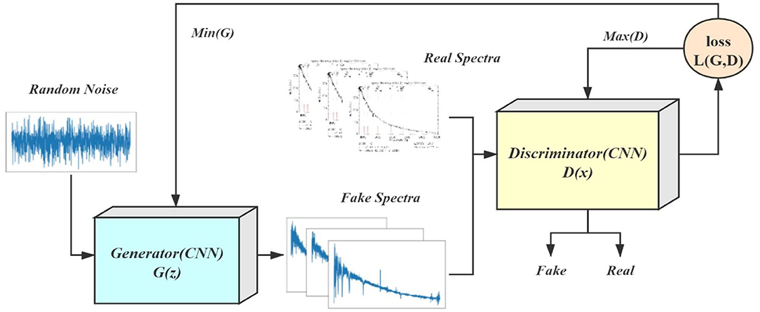
Figure 1. The schematic diagram of LCGAN structure.

Convolutional Neural Network

Artificial neural networks can be seen as stack together with a bunch of layers. They can be divided into the input layer, hidden layers, and output layer. In the hidden layers, we use convolution layers to extract the information of the data.

The convolutional neural network is a kind of neural network which employs a mathematical operation called convolution for processing data. In the convolution layer, we use convolution to capture the features of the input data. The spectra input can be seen as a one-dimensional array of data. In this paper, we use one-dimensional convolution to learn one-dimensional spectral data. This operation is accomplished by the convolution kernel sliding on the data.

For one-dimensional convolution, the convolution kernel starts from the left of the input data and slides on the data in turn from left to right. When the convolution kernel slides to a certain position, the elements of the convolution kernel and the elements of the input data covered by the convolution kernel are multiplied and summed. The formula could be written as the following expression:

$\begin{array}{ll}\begin{array}{c}s(t)={\displaystyle \sum _{i=0}^n}{x}_{t+i}*c_i\end{array}& (2)\end{array}$

where the vector (x₁, …x_t+i, …) represents input data and the i and t represent the position of the data elements. The s is the output data after convolution operation, n represents the length of one-dimensional convolution kernel c, and the vector (c₁, …c_i, …c_n) represents the convolution kernel. An example of a specific operation of one-dimensional convolution is shown in in the first dotted line box in Figure 2.

FIGURE 2

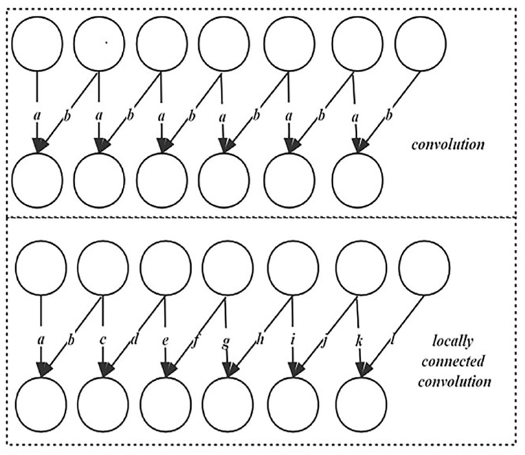
Figure 2. The comparison between a locally connected convolution layer and a convolution layer.

Convolution can be seen as linear matrix multiplication. In the convolution layer, a bias value b will be added to the result after the convolution operation. Then the convolution layers use a nonlinear activation function f(*) to improve the representation ability of the model; the operation of the whole convolution layer is shown in the formula:

$\begin{array}{ll}\begin{array}{c}y(t)=f\left({\displaystyle \sum _{i=0}^n}{x}_{t+i}*c_i+b\right)\end{array}& (3)\end{array}$

f(•) represents the nonlinear activation function. Activation functions decide whether a neuron should be activated or not by calculating the weighted sum and further adding bias with it. They are differentiable operators to transform input signals to outputs, while most of them add non-linearity. We choose the ReLU function and leaky ReLU function to activate the convolution result. ReLU provides a simple non-linear transformation. The formula is shown as:

$\begin{array}{ll}\begin{array}{c}ReLU(x)=max(x,0)\end{array}& (4)\end{array}$

For leaky ReLU, given∝∈ [0, 1], x is the data, its definition is:

$\begin{array}{ll}\begin{array}{c}leakyReLU\left(x\right)=\{\begin{array}{c}x,x>0\\ \propto x,x\le 0\end{array}\end{array}& (5)\end{array}$

Leaky ReLU addresses the problem that a neuron might always output a negative value and therefore cannot make any progress since the gradient is 0 (Radford et al., 2016).

Locally Connected Convolution

Compared with convolution, the locally connected convolution kernels of unshared convolution do not share parameters (Huang et al., 2012). When the convolution kernel slides one position, its parameters will change accordingly. Locally connected layers are useful when we know that different information should be a function of a small part of space, and the same features should not occur across all of space. The comparison between a locally connected convolution layer and a convolution layer is shown in the following Figure 2.

When the convolution kernels of the two layers are set to two units, the parameter values of convolution kernels at each position are shared and dynamically adjusted. In the locally connected layer, the convolution kernels will change parameters with the position sliding. In this mechanism, convolution kernels at different positions in the locally connected convolution can generate different features. For example, in generating a face picture from noise vectors, the same convolution kernel can be used to generate features corresponding to eyes in the upper half of the image. When sliding to the lower part of the image, the convolution kernel can be used to generate mouth features correspondingly.

Compared with convolution, locally connected convolution can pay more attention to the generation of features at different positions in the generative task, so we use locally connected convolution to generate spectral features in different bands in the LCGAN.

We can see that after the convolution operation, the length of the output will be shorter than that of the input. For one-dimensional convolution, the length relationship between input and output is as follows:

$\begin{array}{ll}\begin{array}{c}o=\frac{n+2p-f}{s}+1\end{array}& (6)\end{array}$

where n is the length of input data (for two-dimensional data, n * n is the two-dimensional size of input data), p is the size of filling, s is the size of step size, f is the size of convolution kernel, and O is generally the size of output data. If the convolution operation is not filled, the data size will be reduced with each volume layer.

In order to generate spectral data with more feature dimensions from the original low dimensional random noise vector, we use the method of locally connected convolution and up-sampling to expand the dimension of the data layer by layer. The operation is shown in Figure 3.

FIGURE 3

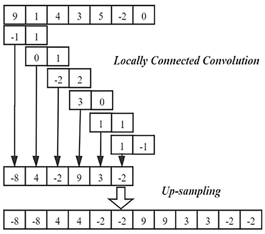
Figure 3. The dimension was expanded by locally connected convolutions and up-sampling.

Generative Adversarial Network

Suppose that there is a simple and easy sampling distribution p(z) in the low dimensional space Z. Generally, p(z) is the standard normal distribution N(0, 1), and the target is the complex distribution X in the high-dimensional space. We want a neural network to fit such a mapping function G:Z → X, which is called generative modeling.

GAN makes the samples generated fit the real data distribution through the adversarial training (Goodfellow et al., 2014; Hong et al., 2019). There are two models in GAN, which can both be made up of deep neural networks. The task of the discriminator model is to distinguish whether the input sample is the real data or the generated data. The goal of the generator model is to generate samples so that the discriminator model cannot distinguish the generated from the true. The training objectives of the two models are the opposite, and they were trained alternately. The training process is similar to a minimax two-player game. The ultimate goal is to generate samples that resemble the real data.

The goal of the discriminator is to distinguish whether a sample is from real data or generated data, so the discriminator model is actually a two-class classifier model. The label y = 1 indicates that the sample comes from real data, and y = 0 indicates that the sample comes from the generator model. The discriminator model should give the probability p(y = 1|x) of the input x from the real distribution. The loss function of the discriminatior is defined as below:

$\begin{array}{ll}\begin{array}{c}\text{min}-(E_x\left[ylogp(y=1|x)+(1-y)logp(y=0|x)\right])\end{array}& (7)\end{array}$

The goal of the generator model is opposite to the discriminator model. The generator aims to let the discriminator distinguish the generated samples as real samples. The generator will minimize the following equation:

$\begin{array}{ll}\begin{array}{c}max\left(E_{z~p(z)}\left[logD(G(z;\theta ))\right]\right)\end{array}& (8)\end{array}$

Above all, for the whole GAN, the loss function can be expressed as follows:

$\begin{array}{ll}\begin{array}{c}\min \max L\left(G,D\right)=E_{x~p\left(x\right)}\left[\log D\left(x;c\right)\right]+\\ E_{z~p\left(z\right)}[\log (1-D(G\left(z;\theta \right);\beta ))]\end{array}& (9)\end{array}$

Here, β is the weight parameter of the discriminator model, θ is the weight parameter of the generative model, D(x; β) is the output of the discriminator model for the input sample x based on weight β, and G(z; θ) is the generated data when the input is Z based on the generator parameterized with weight θ. E[] is the expected operation.

Based on the game theory, the generator model and discriminator model can reach a local Nash equilibrium in theory. For the discriminator model, the probability that any input sample is true is about 0.5. That is, the discriminator model cannot recognize the source of the input sample. At this time, the network can generate samples that conform to the real data distribution.

Our LCGAN architecture is shown in Figure 4.

FIGURE 4

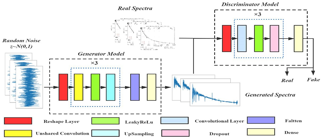
Figure 4. The whole architecture of the LCGAN.

We input a 1 × 900 dimensional random noise vector Z into the generator. Then locally connected convolution with up-sampling mentioned in section locally connected convolution will transform it into a higher dimensional space. Finally, we mix the generated samples with the real O-type samples, and mark them as real or generated. We use them as the training set to train the discriminator model. According to the theory of game theory, when the adversarial training of the two models reaches Nash equilibrium, the samples generated by the generator can be realistic enough. LCGAN generates enough true O-type spectral data to train the recognition model.

In order to train LCGAN model better, we use the following strategies:

(1) Training process optimization of LCGAN. Randomness is helpful to improve the robustness of LCGAN. Training LCGAN is a dynamic process, so the training of LCGAN may be “stuck.” The introduction of randomness in the training process can prevent this situation. We introduce randomness by random dropout of some neural units in the dropout layer (Gal and Ghahramani, 2016; Salimans et al., 2016).

(2) There is a generator model and a discriminator model in LCGAN, and the training promotion of the two models is not consistent. Therefore, it is necessary to control the learning rates of the two models separately. We use two timescale update rules (TTUR) to prevent LCGAN from being dominated by the generator or discriminator (Heusel et al., 2017).

Data Recognition

After the data augmentation, we get the balanced training data set, which can be used to train the recognition model. We built a recognition model based on residual and attention to learn the features of O-type spectra, and finally get an O-type spectra recognition model. In this section, we will describe the techniques in detail.

Residual Networks

In theory, if a new layer is added to the neural network model, the representation ability of the fully trained model will never be lower than the original model. This is because the solution space of the new model is larger than that of the original model, so the new model may obtain a better mapping function to fit the relationship between input and output. For deeper neural networks, if we can train the newly-added layer into an identity function f(x) = x, the new model will be as effective as the original model. As the new model may get a better solution to fit the training data set, the added layer might make it easier to reduce training errors. However, in the actual training, the deeper model often has the problems of gradient dispersion and gradient explosion, which means the model cannot be well-trained.

In the training process of the model, the Error Back Propagation (BP) algorithm is used to transfer the loss backward (Rumelhart et al., 1986). The parameters are adjusted by the chain derivation rule, which requires a continuous propagation gradient. The function of each activation layer of the model is nonlinear rather than identity mapping. Therefore, with the increase of neural network depth, the gradient multiplication will lead to vanishing or exploding in the propagation process.

In order to solve the problems of gradient dispersion and gradient explosion in the deep model, He et al. (2016) proposed the design idea of a residual network. The residual network relies on the idea that every additional layer should be better at containing the identity function as one of its elements. We realize the residual mechanism by the residual block. The structural comparison of the residual block and regular block is shown in Figure 5.

FIGURE 5

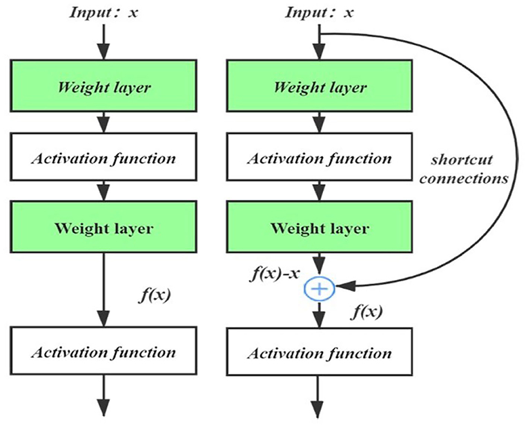
Figure 5. The structural comparison of the residual block and regular block.

When the input is x, we assume that the desired underlying mapping is f(x), which can be used as the input of the next layer. On the left of Figure 5, the regular block structure must learn the mapping f(x). On the right of Figure 5, in the residual structure, the corresponding layer of the neural network only needs to learn the residual mapping: f(x) − x. For example, if we want a layer to learn the identity mapping: f(x)−x, the residual mapping is easier to learn by pushing the weights and biases within the dotted-line box to zero.

The gradient transferred backward from the next layer can be directly transferred to the upper layer through shortcut connections, instead of multiplying activation functions between convolution layers, so that the gradient will not vanish and explode (Orhan and Pitkow, 2018). At the same time, the introduction of a residual structure can be regarded as an integrated model that transforms the original path between two points into a series of path combinations and achieves a better integration effect by promoting each path in the model to be more independent (Veit et al., 2016).

The residual structure helps us to use the deeper convolution neural network to capture the deeper features of spectral data. From the perspective of astronomical spectral data, the residual structure helps the model to expand the depth of the model, which makes the fitting space of the model more complex. This is in line with the specific characteristics of astronomical spectrum data.

Attention Mechanism

People can receive a large amount of sensory information through visual, auditory, tactile, and other ways in daily life. However, the human brain can work orderly with this external information bombing because it can select a small part of useful information from a large amount of the input information to focus on processing and ignore other information. For example, when we look for someone in a crowd, we focus on the person's face. When we want to count the number of people, we often only focus on the outline of each person. We can also learn from the attention mechanism of the human brain, selecting only the key information to focus on and weakening the process of unimportant information to improve the efficiency of the neural network (Zhao et al., 2020). In the task of spectra recognition, the attention mechanism can also be used to make the neural network focus on the information that can express the specific meaning of the spectra to recognize better (Chen et al., 2017).

In convolution operation, each filter corresponds to the convolution result of a channel. Traditional convolution networks default that these different channels have the same contribution to the subsequent recognition results, but the fact is not the case. Different channels carry different features. Some features contribute more to recognition, some features contribute less, and some features even have negative effects. For example, in the process of light propagation, spectral information will be affected by the atmosphere and other external environments, resulting in noise in some bands, which will affect the extraction of spectral features. Maybe the features collected by a channel are noise features, which will affect the performance of the model. We can get the weight of different channels through channel attention and focus on some specific channels (Wang Q. et al., 2020).

As shown in Figure 6, the attention block can be divided into eight stages. Firstly, a convolution operation is performed on the input spectrum (stage 1), producing c channels (stage 2). Then the MaxPooling and AveragePooling operate on these c channels, producing two vectors $w_c^{Max}$ and $w_c^{averge}$ with lengths of c (stage 3). Then, the two vectors in stage 3 were concatenated to one vector w_c (stage 4). In stage 5, the initial weight W_c is sent to a full-connected layer. After learning and adjustment, the output is the final weight array $w_c^{att}$, which is the attention weight (stage 5). At the ReapeatVector layer, the attention weight is extended to an attention matrix with the shape of (l, c) (stage 6). In stage 7, the output of the attention block y_out was obtained (stage 8), by multiplying the attention matrix with the convolution data from stage 2.

FIGURE 6

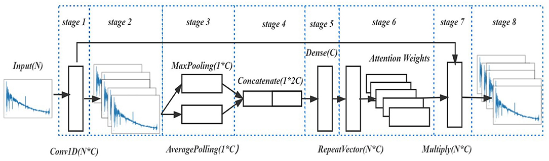
Figure 6. The operations in the attention block.

The attention mechanism helps us to pay more attention to the important bands of the spectra. Through the combination of residual and attention, we built an O-type spectra recognition model by extending the RAC-Net classification model (Zou et al., 2020). After training on the training set, this recognition model could recognize the O-type spectra in the massive spectra.

Results and Discussion

In this section, we will discuss the evaluation criteria and experimental results. We compared our model with SGAN (Zheng et al., 2020) and the recognition model without data augmentation. The experiments show the effect and superiority of our method.

Evaluation

Our model can be divided into two parts: LCGAN for data augmentation and O-type spectra recognition model for recognition. In order to evaluate our model, we refer to the methods in Shmelkov et al., 2018; Wulan et al., 2020; Zou et al., 2020, and adopt three evaluation criteria: GAN-test, GAN-train, and recognition accuracy.

Here, GAN-train is regarded as a kind of diversity measure while GAN-test is an authenticity measure. The higher value of the GAN-train suggests the better diversity of generated data. The higher the value of GAN-test means the more similar between the generated data and the real data. In short, a good generative model must satisfy both diversity and authenticity.

First, to calculate GAN-train, we need to design a convolution classification model and train it with the generated data generated by LCGAN, and then test it on the real data. Suppose the recognition model can learn the corresponding features from the generated data and correctly classify the real data. In those cases, it means that the generated data are similar to the real ones. Second, to calculate GAN-test, we train the classification model on real data and test it on the generated data generated by LCGAN. Finally, we test the recognition accuracy of the O-type spectra recognition model for real data after data augmentation.

Experimental Design

In our experiment, seven different data sets are used. The detailed data composition is as Table 1:

TABLE 1

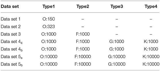
Table 1. The experimental data sets from the LAMOST.

Data set 1 consists of 150 true O-type spectra. The data set is used to train the LCGAN model.

Data set 2 consists of 323 true O-type spectral data.

In Data set 3, a total of 323 true O-type spectra in Data set 2 were up-sampled (duplicated) to obtain 1000 true O-type spectral data. In addition, 1000 spectra of F-types stars were added to Data set 3. Data set 4_a is made up of 4000 spectra, which consists of 1000 generated O-type spectra and real F, G, and K, three classes of 1000 each. The difference between the Data set 4_a and Data set 4_b is that the first O-type spectra are generated by LCGAN, and the second is generated by SGAN.

In the same way, Data set 5_a and Data set 5_b consist of 10000 generated O-type spectra, 10000 F-type spectra, 10000 G-type spectra, and 10000 K-type spectra. We compare our generative model with SGAN (Zheng et al., 2020).

In our experiment, we use two evaluation criteria (GAN-test and GAN-test) in section evaluation to analyze the data augmentation models. This is because GAN-test needs to use real data to train the recognition model, and then use the trained model to test the quality of the generated data. While our real O-type data scale is not enough to train a deep neural network model, so we use the support vector machine (SVM) (Pisner and Schnyer, 2019) as the GAN-train and GAN-test classification model. At the same time, we test the accuracy of the recognition model after data augmentation and without data augmentation.

Results

Experiment Settings

The Keras deep learning framework is used for constructing our LCGAN and O-type spectra recognition model. The CPU we use is Intel E5-2690 v4 (2.60 GHz), the memory is 128G, and the GPU is NVIDIA Tesla K40C/12.00GB.

In the generative model, we used RMSprop with an initial learning rate 0.0001 in the generator, while the learning rate in the discriminator is 0.00015. In the recognition model, we used Adam with an initial learning rate of 0.0001. We use sklearn.svm.NuSVC api to build the SVM model, in which the Gaussian kernel is used as the kernel. The parameter setting of SGAN can be seen in the paper (Zheng et al., 2020).

Experiments on Data Augmentation

In order to calculate the GAN-train and GAN-test, we construct the SVM model for O-type spectra binary recognition (Pisner and Schnyer, 2019). We use Data set 3 to train the SVM model and then test on spectra in Data set 4 to calculate the GAN-test. We use Data set 4 as a training set and then test the SVM model with Data set 2 to calculate GAN-train.

Because the training of the GAN is a dynamic process, different from the general deep neural network, every step of training in the GAN model will change the gradient space (Shmelkov et al., 2018). Meanwhile, the loss of the GAN model cannot prove the quality of data generated by the GAN, so we do not discuss the loss of the GAN. We test the results of multiple rounds of iteration for each model by GAN-test and GAN-train. After analyzing the results of multiple rounds, we get the average value. The final experimental results are as Table 2.

TABLE 2

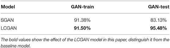
Table 2. The GAN-train and GAN-test results of the SGAN and the LCGAN model.

It can be seen that the scores of the GAN-train and GAN-test of our model are higher than the SGAN model. The GAN-train of LCGAN can reach 91.50% and SGAN can reach 91.38%. The higher the GAN-train, the more likely it is that the data generated by the model will contain more types of real data. It shows the high diversity of the two generative model. The GAN-test of LCGAN can reach 95.48%, which is 12.35% higher than SGAN. It shows that the authenticity of the O-type data generated by LCGAN is better.

Compared with SGAN, LCGAN introduces TTUR to control the confrontation training of generator and discriminator, which can alleviate the problem of mode collapse in the GAN network. So the generator can learn the features of real data and generate more diverse data. Locally connected layers are useful to help the model to generate appropriate spectral features in the different bands. So, the LCGAN can generate more similar spectra.

Experiments on O-type Spectra Recognition Model

The previous experiments show that our data enhancement model has certain advantages in the diversity and authenticity of the generated data. Next, we will build a recognition model and test whether our model can recognize the real O-type spectrum.

We train the O-type spectra recognition model on the generated data set and then test the recognition model's accuracy on the validation set. We use Data set 5, which is composed of O-type spectra generated by two generative models, as the training set of our recognition model. We divide the Data set 5 into the training set and test set according to 7:3. When the test set's loss does not drop after five rounds, we stop the training. We use this method to avoid the recognition model overfitting. At the same time, we use Data set 1 as the O-type data training set to test the accuracy of the recognition model without data augmentation.

To test the performance of the model on real data sets, we take Data set 2 as our validation set to test whether the recognition model can recognize the real O-type spectral data. LCGAN and SGAN have been trained for more than 2,000 iterations, and we sampled them on multiple iterations. In the previous work, we only tested GAN-train and GAN-test on SVM, and the data only had two types: O-type and F-type. When testing the O-type spectra recognition model, we expand the types of data sets and expanded the types of data to O, F, G, and K. We conducted 10 experiments in each group and took the median as the final result. The results can be seen in Figure 7.

FIGURE 7

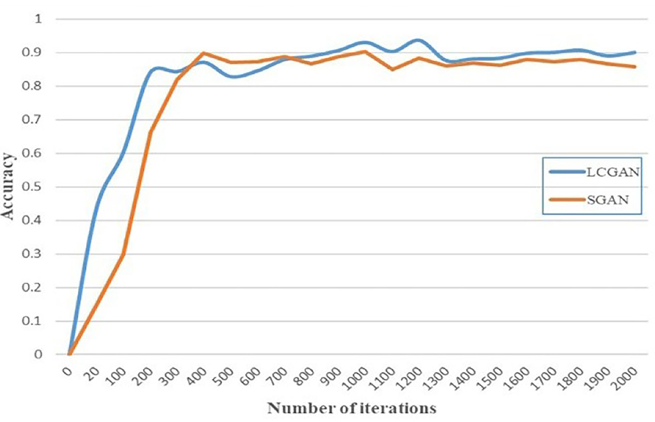
Figure 7. Based on the data generated by the LCGAN and SGAN of different iterations, the accuracy of the O-type spectra recognition model on the validation set.

Because the GAN model has the problem of mode collapse, if the generator repeatedly imitates a piece of data in the real data, the discriminator will always judge it as true. Simultaneously, after reaching the local equilibrium, the dynamic gradient space makes it possible for the model due to more training. It can be seen that the accuracy of the two models will oscillate after reaching the highest accuracy.

The recognition accuracy of the recognition model without data augmentation is 85.1% (Zou et al., 2020). Compared with the recognition model after data augmentation by LCGAN or SGAN, the accuracy of the recognition model without data augmentation is lower. Comparing the two models, the LCGAN model has the following advantages: in terms of the overall effect, the average and highest accuracy rate that LCGAN can achieve is higher than that of SGAN. The accuracy rate of LCGAN can reach 93.67%, which is 3.31% higher than SGAN.

Compared to the LeNet-like architecture classification model used by Zheng et al. (2020), we build the O-type spectra recognition model with the attention mechanism and the residual structure. The attention mechanism helps the recognition model to pay attention to the important spectral band, reducing the influence of invalid information (such as noise). The residual structure helps the recognition model to deepen the depth and improve the representation ability of the network.

The experimental results show that spectra recognition model based on data augmentation can complete the task of O-type spectra recognition.

Conclusion

In this paper, we propose a novel model LCGAN to complete the data augmentation task by introducing a generative adversarial network and locally connected convolution. Then, we extend an O-type spectra recognition model based on residual and attention mechanisms. Base on the LCGAN, the O-type spectra recognition model can learn the features of O-type spectra. The above results show that our O-type spectra recognition model based on data augmentation has some advantages over other models in the task of O-type spectra recognition.

Compared with Zheng et al. (2020), on the one hand, we improve the data augmentation model based on GAN; on the other hand, we introduce attention mechanism and residual structure into the recognition model, which improves the learning ability of the recognition model. Compared with Zou et al. (2020), we pay more attention to the data enhancement of rare stars. The data-driven neural network classification and recognition method cannot deal with the recognition task of rare stars well. Our method has certain feasibility and superiority in dealing with the recognition and classification of these rare stars.

However, our model still has some problems in explaining the features of the generated spectra. This is because the GAN relies on the adversarial training between the generator and the discriminator. GAN generates spectra by reducing the distance between the distribution of generated samples and the distribution of real samples. The model is not enough to explain the features of the generated spectra. In future work, we will focus on the exploration of the generated spectral features.

Data Availability Statement

Publicly available datasets were analyzed in this study. This data can be found at: http://dr7.lamost.org/; http://www.lamost.org/dr8/.

Author Contributions

All authors listed have made a substantial, direct and intellectual contribution to the work, and approved it for publication.

Funding

This work was supported by National Key R&D Program of China (No. 2019YFA0405502) and the National Science Foundation of China (No. U1931209).

Conflict of Interest

The authors declare that the research was conducted in the absence of any commercial or financial relationships that could be construed as a potential conflict of interest.

The reviewer JZ declared a shared affiliation with one of the authors, K-FW, to the handling editor at time of review.

Acknowledgments

The authors would like to acknowledge Guoshoujing Telescope. Guoshoujing Telescope (the Large Sky Area Multi-Object Fiber Spectroscopic Telescope, LAMOST) is a National Major Scientific Project built by the Chinese Academy of Sciences. Funding for the project has been provided by the National Development and Reform Commission. LAMOST is operated and managed by the National Astronomical Observatories, Chinese Academy of Sciences.

Footnotes

1. ^Available online at: http://www.restfmri.net.

References

Ai, Y. L., Wu, X.-B., Yang, J., Yang, Q., Wang, F., Guo, R., et al. (2016). The large sky area multi-object fiber spectroscopic telescope quasar survey: quasar properties from the first data release. Am. Astronom. Soc. J. 151:24. doi: 10.3847/0004-6256/151/2/24

CrossRef Full Text | Google Scholar

Chen, L., Zhang, H., Xiao, J., Nie, L., Shao, J., Liu, W., et al. (2017). “SCA-CNN: spatial and channel-wise attention in convolutional networks for image captioning,” in Proceedings - 30th IEEE Conference on Computer Vision and Pattern Recognition, CVPR 2017 Vol. 1 (Honolulu, HI), 6298–6306. doi: 10.1109/CVPR.2017.667

CrossRef Full Text

Cubuk, E. D., Zoph, B., Mane, D., Vasudevan, V., and Le, Q. V. (2019). “Autoaugment: learning augmentation strategies from data,” in Proceedings of the IEEE Computer Society Conference on Computer Vision and Pattern Recognition (Long Beach, CA), 113–123. doi: 10.1109/CVPR.2019.00020

CrossRef Full Text | Google Scholar

Cui, X. Q., Zhao, Y. H., Chu, Y. Q., Li, G. P., Li, Q., Zhang, L. P., et al. (2012). The large sky area multi-object fiber spectroscopic telescope (LAMOST). Res. Astronom. Astrophys. 12, 1197–1242. doi: 10.1088/1674-4527/12/9/003

CrossRef Full Text | Google Scholar

Gal, Y., and Ghahramani, Z. (2016). “Dropout as a Bayesian approximation: representing model uncertainty in deep learning,” in 33rd International Conference on Machine Learning, ICML 2016, Vol. 48 (New York, NY), 1050−1059.

Google Scholar

Goodfellow, I. J., Pouget-Abadie, J., Mirza, M., Xu, B., Warde-Farley, D., Ozair, S., et al. (2014). “Generative adversarial nets,” in Proceedings of the 27th International Conference on Neural Information Processing Systems, Vol. 2 (Montréal, QC: Palais des Congrès de Montréal), 2672–2680.

Google Scholar

He, K., Zhang, X., Ren, S., and Sun, J. (2016). “Deep residual learning for image recognition,” in Proceedings of the IEEE Computer Society Conference on Computer Vision and Pattern Recognition. Vol. 1 (Las Vegas, NV), 770–778. doi: 10.1109/CVPR.2016.90

PubMed Abstract | CrossRef Full Text | Google Scholar

Heusel, M., Ramsauer, H., Unterthiner, T., Nessler, B., and Hochreiter, S. (2017). “GANs trained by a two time-scale update rule converge to a local Nash equilibrium,” in Proceedings of the 31st International Conference on Neural Information Processing Systems (Red Hook, NY: Curran Associates Inc.), 6629–6640.

Google Scholar

Hong, Y., Hwang, U., Yoo, J., and Yoon, S. (2019). How generative adversarial networks and their variants work: an overview. ACM Comput. Surveys. 52, 1–43. doi: 10.1145/3301282

CrossRef Full Text | Google Scholar

Hou, W., Luo, A., Yang, H., Wei, P., Zhao, Y., Zuo, F., et al. (2015). A large sample of metallic-line star candidates from LAMOST Data Release 1. Monthly Notices Royal Astronom. Soc. 449, 1401–1407. doi: 10.1093/mnras/stv176

CrossRef Full Text | Google Scholar

Huang, G. B., Lee, H., and Learned-Miller, E. (2012). “Learning hierarchical representations for face verification with convolutional deep belief networks,” in Proceedings of the IEEE Computer Society Conference on Computer Vision and Pattern Recognition (Providence, RI), 2518–2525. doi: 10.1109/CVPR.2012.6247968

CrossRef Full Text | Google Scholar

Kong, X., Luo, A. L., Li, X. R., Wang, Y. F., Li, Y. B., and Zhao, J. K. (2018). Spectral feature extraction for DB white dwarfs through machine learning applied to new discoveries in the Sdss DR12 and DR14. Publ. Astronom. Soc. Pacific 130:084203. doi: 10.1088/1538-3873/aac7a8

CrossRef Full Text | Google Scholar

Li, X. R., Liu, Z. T., Hu, Z. Y., Wu, F. C., and Zhao, Y. H. (2007). Celestial spectrum flux standardization for classification. Spectroscopy Spectr. Anal. 27, 1448–1451.

PubMed Abstract | Google Scholar

Li, Y.-B., Luo, A.-L., Du, C.-D., Zuo, F., Wang, M.-X., Zhao, G., et al. (2018). Carbon stars identified from LAMOST DR4 using machine learning. Astrophys. J. Suppl. Ser. 234:31. doi: 10.3847/1538-4365/aaa415

CrossRef Full Text | Google Scholar

Müller, R., Kornblith, S., and Hinton, G. (2019). “When does label smoothing help?” in Advances in Neural Information Processing Systems, Vol. 32. Available online at: https://proceedings.neurips.cc/paper/2019/file/f1748d6b0fd9d439f71450117eba2725-Paper.pdf (accessed June 10, 2020).

Google Scholar

Orhan, A. E., and Pitkow, X. (2018). “Skip connections eliminate singularities,” in 6th International Conference on Learning Representations, Conference Track Proceedings. Available online at: https://openreview.net/forum?id=HkwBEMWCZ (accessed February 21, 2018).

Google Scholar

Perryman, M. A. C., De Boer, K. S., Gilmore, G., Høg, E., Lattanzi, M. G., Lindegren, L., et al. (2001). GAIA: composition, formation and evolution of the Galaxy. Astronom. Astrophys. 369, 339–363. doi: 10.1051/0004-6361:20010085

CrossRef Full Text | Google Scholar

Pisner, D. A., and Schnyer, D. M. (2019). “Support vector machine,” in Machine Learning: Methods and Applications to Brain Disorders (Academic Press), 101–121. doi: 10.1016/B978-0-12-815739-8.00006-7

CrossRef Full Text | Google Scholar

Qin, L., Luo, A.-L., Hou, W., Li, Y.-B., Zhang, S., Wang, R., et al. (2019). Metallic-line stars identified from low-resolution spectra of LAMOST DR5. Astrophys. J. Suppl. Ser. 242:13. doi: 10.3847/1538-4365/ab17d8

CrossRef Full Text | Google Scholar

Radford, A., Metz, L., and Chintala, S. (2016). “Unsupervised representation learning with deep convolutional generative adversarial networks,” in 4th International Conference on Learning Representations, ICLR 2016 - Conference Track Proceedings. Available online at: https://arxiv.org/abs/1511.06434 (accessed January 7, 2016).

Google Scholar

Rumelhart, D. E., Hinton, G. E., and Williams, R. J. (1986). Learning representations by back-propagating errors. Nature 323, 533–536. doi: 10.1038/323533a0

CrossRef Full Text | Google Scholar

Salimans, T., Goodfellow, I., Zaremba, W., Cheung, V., Radford, A., and Chen, X. (2016). “Improved techniques for training GANs,” in Advances in Neural Information Processing Systems, Vol. 29, 2234–2242. doi: 10.5555/3157096.3157346

CrossRef Full Text | Google Scholar

Shmelkov, K., Schmid, C., and Alahari, K. (2018). How good is my GAN? Lecture Notes Eur. Conf. Comp. Vis. 11206, 218–234. doi: 10.1007/978-3-030-01216-8_14

CrossRef Full Text | Google Scholar

Shorten, C., and Khoshgoftaar, T. M. (2019). A survey on image data augmentation for deep learning. J. Big Data. 6, 1–48. doi: 10.1186/s40537-019-0197-0

CrossRef Full Text | Google Scholar

Vaswani, A., Shazeer, N., Parmar, N., Uszkoreit, J., Jones, L., Gomez, A. N., et al. (2017). “Attention is all you need,” in Advances in Neural Information Processing Systems (Long Beach, CA: Curran Associates Inc.), 6000–6010. doi: 10.5555/3295222.3295349

CrossRef Full Text | Google Scholar

Veit, A., Wilber, M., and Belongie, S. (2016). Residual networks behave like ensembles of relatively shallow networks. Adv. Neural Inform. Process. Syst. 29, 550–558. Available online at: https://proceedings.neurips.cc/paper/2016/hash/37bc2f75bf1bcfe8450a1a41c200364c-Abstract.html

Google Scholar

Wang, Q., Wu, B., Zhu, P., Li, P., Zuo, W., and Hu, Q. (2020). “ECA-Net: efficient channel attention for deep convolutional neural networks,” in Proceedings of the IEEE Computer Society Conference on Computer Vision and Pattern Recognition (Seattle, WA), 11531–11539. doi: 10.1109/CVPR42600.2020.01155

CrossRef Full Text

Wang, Y., Yao, Q., Kwok, J. T., and Ni, L. M. (2020). Generalizing from a few examples: a survey on few-shot learning. ACM Comput. Surveys. 53, 1–34. doi: 10.1145/3386252

CrossRef Full Text | Google Scholar

Wulan, N., Wang, W., Sun, P., Wang, K., Xia, Y., and Zhang, H. (2020). Generating electrocardiogram signals by deep learning. Neurocomputing 404, 122–136. doi: 10.1016/j.neucom.2020.04.076

CrossRef Full Text | Google Scholar

York, D. G., Adelman, J., Anderson, J. E. Jr, Anderson, S. F., Annis, J., Bahcall, N. A., et al. (2000). The sloan digital sky survey: technical summary. Astronom. J. 120, 1579–1587. doi: 10.1086/301513

CrossRef Full Text | Google Scholar

Zhao, G., Zhao, Y. H., Chu, Y. Q., Jing, Y. P., and Deng, L. C. (2012). LAMOST spectral survey - an overview. Res. Astronom. Astrophys. 12, 723–734. doi: 10.1088/1674-4527/12/7/002

CrossRef Full Text | Google Scholar

Zhao, H., Jia, J., and Koltun, V. (2020). “Exploring self-attention for image recognition,” in Proceedings of the IEEE Computer Society Conference on Computer Vision and Pattern Recognition (Seattle, WA), 10073–10082. doi: 10.1109/CVPR42600.2020.01009

CrossRef Full Text | Google Scholar

Zheng, Z. P., Qiu, B., Luo, A. L., and Li, Y. B. (2020). Classification for unrecognized spectra in lamost dr6 using generalization of convolutional neural networks. Publ. Astronom. Soc. Pacific 132:024504. doi: 10.1088/1538-3873/ab5ed7

CrossRef Full Text | Google Scholar

Zou, Z., Zhu, T., Xu, L., and Luo, A.-L. (2020). Celestial spectra classification network based on residual and attention mechanisms. Publ. Astronom. Soc. Pacific 132:044503. doi: 10.1088/1538-3873/ab7548

CrossRef Full Text | Google Scholar