Circumbinary Habitable Zones in the Presence of a Giant Planet

1. Introduction

Over the past three decades exoplanet researchers have discovered more than four thousands planets outside our Solar System¹. Improvements in detection techniques have now reached a point where finding planets of similar size to our Earth has become a reality. Four of the planets in the Trappist-1 system (Gillon et al., 2016) or TOI-700d (Gilbert et al., 2020; Rodriguez et al., 2020) are prime examples. Several planets in those systems orbit their host star inside the habitable zone. The habitable zone is the region where a terrestrial planet on a circular orbit about its host star can support liquid water on its surface (Kasting et al., 1993). A number of planets have been found to reside in binary stars systems, some of which even orbit both stars (e.g., Doyle et al., 2011; Welsh et al., 2012; Kostov et al., 2014). We refer to the latter as circumbinary planets. Unresolved questions regarding the formation and dynamical evolution of such systems (Marzari and Thebault, 2019) have motivated a number of studies in recent years, particularly on whether or not such systems could host potentially habitable worlds (Haghighipour and Kaltenegger, 2013; Kane and Hinkel, 2013; Cuntz, 2014, 2015; Forgan, 2014; Jaime et al., 2014; Cukier et al., 2019; Shevchenko et al., 2019; Yadavalli et al., 2020). Some of the challenges in assessing habitability in binary star systems arises from the fact that one has to account for two sources of radiation, possibly of different spectral type. Moreover, the distance of the planet to each star keep changing over time in a non-trivial manner due to gravitational interactions between the planet and the two stars.

The introduction of “dynamically informed habitable zones" allowed Eggl et al. (2012) to study the prospects for habitability of planets orbiting a single star in a binary star system. Dynamically informed habitable zones for systems with a potentially habitable world on a circumbinary orbit were developed in Eggl (2018) and Eggl et al. (2020). In this work, we improve on previous analytic estimates for circumbinary dynamically informed habitable zones and extend the concept to systems that are known to host an additional giant planet. Here we refer to giant planets as bodies with masses ranging from Neptune mass up to a few Jupiter masses.

The structure of this paper is as follows: in the next section we explain the general principles behind dynamically informed habitable zones and construct the required tools to extend the concept to include a giant planet in the system. In section 3 we investigate the potential of binary star systems with known circumbinary planets observed during the Kepler mission (e.g., Doyle et al., 2011; Welsh et al., 2012; Kostov et al., 2014) to host additional potentially habitable worlds. Finally, in section 4 we summarize and discuss the work presented here.

2. Dynamically Informed Habitable Zones

The nearly circular orbit of the Earth around the Sun ensures that the planet receives an almost constant amount of radiation on a permanent basis. That assumption falters for a circumbinary planet, however. The second star provides an additional source of radiation, and more importantly, it is also a source of gravitational perturbations for the planetary orbit. Even if a planet is on an initially circular orbit around the binary, the orbit will become elliptic over time (see e.g., Georgakarakos, 2009; Georgakarakos and Eggl, 2015). As a consequence, the planet experiences time dependent irradiation. Depending on how effectively the climate on the planet can buffer changes in incoming radiation its response to radiative forcing can differ widely (see e.g., Popp and Eggl, 2017; Way and Georgakarakos, 2017; Haqq-Misra et al., 2019; Wolf et al., 2020). In order to capture the various responses defined by a planet's climate inertia, we make use of so-called “dynamically informed habitable zones” (DIHZs) (see e.g., Georgakarakos et al., 2018). DIHZs not only take the orbital evolution of the planet around the binary into account, but they can even trace habitable zone limits for different climate inertia values a planet may have. Climate inertia is defined as the time it takes climate parameters, such as the mean surface temperature, to react to radiative forcing. The faster the mean surface temperature changes, the lower the climate inertia of a planet is.

In order to account for the effect of climate inertia, we follow the general methodology as outlined in (Eggl et al., 2012) and (Georgakarakos et al., 2018) and introduce three different DIHZs: the permanently habitable zone (PHZ), the averaged habitable zone (AHZ), and the extended habitable zone (EHZ). The PHZ is the most conservative region. For a planet to reside in the PHZ means that it stays continuously within habitable insolation limits in spite of orbit-induced variability. In other words, the PHZ is the region where a planet with essentially zero climate inertia could remain habitable on stellar evolution timescales. On the other end of the spectrum is the averaged habitable zone, where a planet is assumed to buffer all variations in irradiation and remains habitable as long as the insolation average stays within habitable limits. This scenario corresponds to a planet with a very high climate inertia.

The extended habitable zone lies between the above extremes by assuming that the planetary climate has limited buffering capabilities. The EHZ is defined as the region where the planet stays on average plus minus one standard deviation within habitable insolation limits. In order to calculate DIHZ borders for circumbinary systems, we need to understand (a) whether or not a configuration is dynamical stable, (b) how the orbital evolution of the system affects the amount of radiation the planet receives, and (c) how the combined quantity and spectral distribution of the star light influences the climate of a potentially habitable world.

2.1. Dynamical Stability

Dynamical stability is a necessary condition for habitability of a circumbinary planet. If a planet is ejected from a system, water that may be present on its surface will ultimately freeze. There are a number of ways to predict whether or not a potentially habitable world is on a stable orbit (e.g., see Georgakarakos, 2008). In this work, we make use of the empirical condition developed in Holman and Wiegert (1999) which provides critical semi-major axis values below which planetary orbits around binary stars become unstable. The critical semi-major axis in a circumbinary system depends on the eccentricity, semi-major axis, and mass ratio of the binary as can be seen from the following equation:

$\begin{array}{l}{a}_c=[(1.60\pm 0.04)+(5.10\pm 0.05)e_b+(-2.22\pm 0.11)e_b^2\\ +(4.12\pm 0.09)\mu +(-4.27\pm 0.17)e_b\mu +(-5.09\pm 0.11){\mu }^2\\ +(4.61\pm 0.36)e_b^2{\mu }^2]a_b,& (1)\end{array}$

where a_b is the semi-major axis of the binary, e_b is the eccentricity of the binary and μ = m₂/(m₁ + m₂); m₁ and m₂ are the masses of the two stars (m₁ > m₂ without loss of generality). A value of planetary semi-major axis below a_c indicates that the planet will escape from the system or collide with one of the stars.

Once we confirm that a potentially habitable planet is on a stable orbit, we can proceed to investigate how much radiation it receives from the two stars. The latter depends on the orbit of the planet which evolves over time. By modeling the evolution of the stellar and planetary orbits we can estimate the actual amount and spectral composition of the radiation the planet receives. To this end we make use of an analytic orbit propagation technique for circumbinary planets developed in Georgakarakos and Eggl (2015).

2.2. The Classical Habitable Zone

For systems consisting of a star and a terrestrial planet on a fixed circular orbit, the limits of the classical habitable zone (CHZ) read

$\begin{array}{ll}{r}_I={\left(\frac{L}{S_I}\right)}^{\frac{1}{2}}\text{ and }{r}_O={\left(\frac{L}{S_O}\right)}^{\frac{1}{2}},& (2)\end{array}$

where r is the distance of the planet to its host star in astronomical units, L is the host star's luminosity in solar luminosities, and S_I and S_O are effective insolation values or “spectral weights" (Kasting et al., 1993). The latter correspond to the number of solar constants that trigger a runaway greenhouse process (subscript I) evaporating surface oceans, or a snowball state (subscript O) freezing oceans on a global scale. Spectral weights are functions of the effective temperature of the host star and, therefore, they take the specific wavelength distribution of a star's light into account. They can be calculated by the expressions below which can be found in Kopparapu et al. (2014):

$\begin{array}{l}{S}_I=1.107+1.332·10^{-4}{T}_c+1.580·10^{-8}{T}_c^2\\ \begin{array}{ll}-& 8.308·10^{-12}{T}_c^3-1.931·10^{-15}{T}_c^4\end{array}& (3)\end{array}$

$\begin{array}{l}{S}_O=0.356+6.171·10^{-5}{T}_c+1.698·10^{-9}{T}_c^2\\ \begin{array}{ll}-& 3.198·10^{-12}{T}_c^3-5.575·10^{-16}{T}_c^4.\end{array}& (4)\end{array}$

T_c = T_eff/1K − 5780, with T_eff being the effective temperature of the star, while the value of 5780 used in the above fit formulae corresponds to the effective temperature T_⊙ of the Sun. The coefficients in Equations (3) and (4) refer to a planet of one Earth mass but similar functions are available for different terrestrial planet masses. In case stellar luminosities have not been observed directly, one can use stellar radii R_* and effective temperatures T_eff instead:

$\begin{array}{l}\frac{L}{L_{\odot }}={\left(\frac{R_{*}}{R_{\odot }}\right)}^2{\left(\frac{T_{eff}}{T_{\odot }}\right)}^4,\end{array}$

where R_⊙ is the radius of the Sun.

2.3. The Permanently Habitable Zone

We will now use the above concepts to determine the permanently habitable zone. In order to find the borders of the region wherein the planet stays always within habitable insolation limits, i.e., the PHZ, we need to find the effective insolation extrema a circumbinary planet is likely to encounter. In hierarchical systems of two stars and a circumbinary planet, the planetary semi-major axis remains practically constant over time. In addition, if a system is coplanar, the time evolution of the eccentricity vectors determines the geometric configuration at any given moment. Assuming furthermore that the gravitational effect of the planet on the stellar binary is negligible, maximum and minimum insolation configurations are determined through the maximum planetary eccentricity $e_p^{max}$. We use the expressions derived in Georgakarakos and Eggl (2015) that allow us to calculate $e_p^{max}$ as a function of initial conditions and system parameters. The apocenter and pericenter distance between the planet and the barycenter of the binary star can in turn be expressed through the maximum eccentricity as well as the semi-major axis of the planetary orbit a_p, i.e., $Q_p=a_p(1+e_p^{max})$ and $q_p=a_p(1-e_p^{max})$. Figure 1 is a schematic representation of our system, meant to help the reader visualize configurations that lead to insolation extrema. The planet receives maximum insolation when it is at pericenter with respect to the binary barycenter and closer to the brighter star, i.e., when the angle ϕ between the line that connects the stars and the line that connects the planet to the binary barycenter is ϕ = 0°. Thus, the three bodies are aligned and the mathematical expression that determines the inner edge of the PHZ is

$\begin{array}{ll}PH{Z}_I:\frac{L_1}{S_{1,I}{(q_p-\mu Q_b)}^2}+\frac{L_2}{S_{2,I}{\left[q_p+(1-\mu )Q_b\right]}^2}\le 1,& (5)\end{array}$

where Q_b= a_b(1+e_b). Note that we have normalized the stellar luminosities with their respective spectral weights in order to account for the effect of each star's individual spectral energy distribution on the planetary climate. The minimum insolation configuration is not as straight forward to determine. If one star is substantially more massive and luminous than the other a minimum can be reached when the brighter star is farthest from the planet and the planet is at apocenter with respect to the barycenter of the binary star. This is the case when ϕ = 180° which corresponds to the following condition for the outer edge of the PHZ

$\begin{array}{ll}PH{Z}_O:\frac{L_1}{S_{1,O}{(Q_p+\mu Q_b)}^2}+\frac{L_2}{S_{2,O}{[Q_p-(1-\mu )Q_b]}^2}\ge 1,& (6)\end{array}$

If we have two stars of equal mass, then the minimum radiation configuration is reached when ϕ = 90°. Hence, the minimum insolation condition in this case is

$\begin{array}{ll}PH{Z}_O:\frac{1}{Q_p^2+0.5Q_b^2}\left(\frac{L_1}{S_{1,O}}+\frac{L_2}{S_{2,O}}\right)\ge 1.& (7)\end{array}$

When the mass ratio of the binary is close to–but not exactly–equal to one (with m₁ > m₂) and the planet is located at a suitable distance, the minimum insolation geometry occurs between ϕ = 90° and ϕ = 180°. Figure 2 illustrates this behavior for a variety of binary mass ratios. We note, however that the difference in insolation received by the planet between said configurations is small (~10%). We limit our approach to comparing the perpendicular and straight line configurations and use the one that provides the smallest value. Consequently the minimum insolation condition for the outer border of the PHZ reads

$\begin{array}{l}PH{Z}_O:min\{\frac{L_1}{S_{1,O}{(Q_p+\mu Q_b)}^2}+\frac{L_2}{S_{2,O}{[Q_p-(1-\mu )Q_b]}^2},\\ \frac{L_1}{S_{1,O}(Q_p^2+{\mu }^2{Q}_b^2)}+\frac{L_2}{S_{2,O}[Q_p^2+{(1-\mu )}^2{Q}_b^2]}\}\ge 1.& (8)\end{array}$

One can find the numeric values for the borders of the PHZ by solving Equations (5) through (8) for a_p.

FIGURE 1

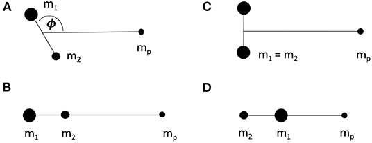
Figure 1. A schematic representation of possible binary star - planet geometries representing irradiation minima: (A–C) and maxima (D) for various mass ratios of the binary star (m₂/m₁). A standard mass-luminosity relation for main sequence stars is assumed. The more massive star is m₁, the less massive star is m₂, and the planet is represented by m_p.

FIGURE 2

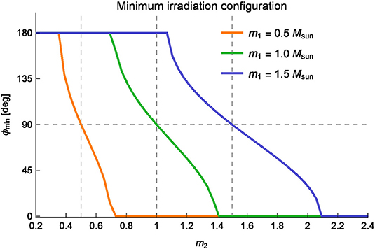
Figure 2. Angle ϕ_min for the minimum planetary insolation configuration against the mass of the secondary star m₂ for various masses of the primary star m₁. We assume a planet on a circular orbit at a distance of 2.37au from the binary barycenter, while the binary stars are evolved on a circular orbit with a semi-major axis of 1au.

We would like to point out here that for all the above insolation extrema configurations we have assumed that the stars are point masses. In reality, however, the stars have finite sizes. Depending on the distance between the two stars and on the distance between the planet and the binary, it is possible that when the three bodies are aligned the planet may receive reduced insolation due to the eclipsed star. In such a scenario, the minimum insolation configuration (Figure 1C) will still be valid. On the other hand, the maximum insolation configuration (Figure 1D) would provide a smaller insolation value. Wolf et al. (2020) have shown, however, that eclipses have little effect on the overall stability of the climate. But even if the insolation change is considerable, as soon as the three bodies get out of alignment, the planet will then receive near maximum insolation. Hence, Equation (5) constitutes a reasonable approximation for our purposes.

2.4. The Averaged Habitable Zone

The averaged habitable zone is the region around a binary star where a planet remains habitable inspite of variations in irradiation. That is, as long as the insolation average is compatible with habitable limits a planet with a high climate inertia can remain potentially habitable. The averaged over time radiation that a planet receives when orbiting a single star is

$\begin{array}{ll}\langle S\rangle =\frac{1}{P}{\displaystyle {\int }_0^P}\frac{L}{r_p^2(t)}dt=\frac{n_p}{2\pi }{\displaystyle {\int }_0^{2\pi }}\frac{Ld{f}_p}{n_p{a}_p^2\sqrt{1-e_p^2}}=\frac{L}{a_p^2\sqrt{1-e_p^2}},& (9)\end{array}$

where L is the stellar luminosity, P the period of the planetary motion, n_p is the mean motion of the planet, f_p is its true anomaly, and r_p the distance between the source of radiation and the planet; we made use of the well-known relation $r_p^{2}d{f}_p/dt=n_p{a}_p^2\sqrt{1-e_p^2}$. We can now extend this simple relation to circumbinary orbits. Assuming that the distance between the two stars is small compared to the distance between the planet and the binary star barycenter, i.e., the orbital period of the binary pair is much smaller than that of the planet, we can approximate the average over time insolation around the binary by placing the two stars at their barycenter and make use of Equation (9). In other words we approximate the three body system as a two-body problem with a central “hybrid star” that has the combined mass, luminosity, and spectral energy distribution of the stellar binary. This leads to

$\begin{array}{ll}\langle S\rangle =\frac{L_1+L_2}{a_p^2\sqrt{1-\langle e_p^2\rangle }},& (10)\end{array}$

where $\langle e_p^2\rangle$ is the averaged square planetary eccentricity over time and initial angles as given in Georgakarakos and Eggl (2015). Under those assumptions the borders of the AHZ are defined through the following inequalities

$\begin{array}{ll}AH{Z}_I:\frac{L_1/S_{1,I}+L_2/S_{2,I}}{a_p^2\sqrt{1-\langle e_p^2\rangle }}\le 1& (11)\end{array}$

and

$\begin{array}{ll}AH{Z}_O:\frac{L_1/S_{1,O}+L_2/S_{2,O}}{a_p^2\sqrt{1-\langle e_p^2\rangle }}\ge 1.& (12)\end{array}$

Note that $\langle e_p^2\rangle$ generally depends on a_p in a non-trivial way. The full expression for $\langle e_p^2\rangle$ along with the expression for $e_p^{max}$ is provided in the Appendix. Once more, solving Equations (11) and (12) for a_p yields the numeric values for the borders of the AHZ.

2.5. The Extended Habitable Zone

The definition of the extended habitable zone in section 2 translates into the following equations:

$\begin{array}{ll}\langle S\rangle +\sigma =S_I\text{ and }\langle S\rangle -\sigma =S_O.& (13)\end{array}$

The standard deviation σ can be found via the insolation variance

$\begin{array}{ll}{\sigma }^2=\langle S^2\rangle -{\langle S\rangle }^2.& (14)\end{array}$

We already have an expression for 〈S〉 from Equation (10), but we are yet to find 〈S²〉. For a planet around a single star, 〈S²〉 is

$\begin{array}{l}\langle S^2\rangle =\frac{1}{P}{\displaystyle {\int }_0^P}\frac{L^2}{r_p^4(t)}dt=\frac{n_p}{2\pi }{\displaystyle {\int }_0^{2\pi }}\frac{{(1+e_p\text{ cos }{f}_p)}^2}{a_p^2{(1-e_p^2)}^2}\\ \begin{array}{l}\frac{L^{2}d{f}_p}{n_p{a}_p^2\sqrt{1-e_p^2}}=\frac{L^2(1+e_p^2/2)}{a_p^4{(1-e_p^2)}^{5/2}}.\end{array}& (15)\end{array}$

Using the same approach that lead to Equation (10), namely combining the stellar binary into a “hybrid star” we can construct a closed analytic expression for 〈S²〉 of a circumbinary planet, namely

$\begin{array}{ll}\langle S^2\rangle =\frac{{(L_1+L_2)}^2(1+\langle e_p^2\rangle /2)}{a_p^4{(1-\langle e_p^2\rangle )}^{5/2}}.& (16)\end{array}$

Combining Equations (10) and (16) and normalizing the individual stellar contributions with the respective spectral weights X_i ∈ {S_i,I, S_i,O}, where i is the index of the respective star, yields:

$\begin{array}{ll}{\sigma }_X^2={\left(\frac{L_1}{X_1}+\frac{L_2}{X_2}\right)}^2\frac{1}{a_p^4(1-\langle e_p^2\rangle )}\left[\frac{1+\langle e_p^2\rangle /2}{{(1-\langle e_p^2\rangle )}^{3/2}}-1\right].& (17)\end{array}$

The inner border of the EHZ is then defined through

$\begin{array}{l}EH{Z}_I:\left(\frac{L_1}{S_{1,I}}+\frac{L_2}{S_{2,I}}\right)\frac{1}{a_p^2\sqrt{1-\langle e_p^2\rangle }}\\ \begin{array}{l}\left\{1+\sqrt{\left[\frac{1+\langle e_p^2\rangle /2}{{(1-\langle e_p^2\rangle )}^{3/2}}-1\right]}\right\}\le 1,\end{array}& (18)\end{array}$

while the outer border is defined via

$\begin{array}{l}EH{Z}_O:\left(\frac{L_1}{S_{1,O}}+\frac{L_2}{S_{2,O}}\right)\frac{1}{a_p^2\sqrt{1-\langle e_p^2\rangle }}\\ \begin{array}{l}\left\{1-\sqrt{\left[\frac{1+\langle e_p^2\rangle /2}{{(1-\langle e_p^2\rangle )}^{3/2}}-1\right]}\right\}\ge 1\end{array}& (19)\end{array}$

Numerical values for the inner and outer EHZ borders can be found via solving the above equations for a_p.

3. Application to Kepler Systems With Known Circumbinary Planets

In order to demonstrate the merit of dynamically informed habitable zones, we apply our method to the Kepler circumbinary planets. For that purpose we select Kepler-16 (Doyle et al., 2011), Kepler-34 and Kepler-35 (Welsh et al., 2012), Kepler-38 (Orosz et al., 2012), Kepler-64 (Schwamb et al., 2013), Kepler-413 (Kostov et al., 2014), Kepler-453 (Welsh et al., 2015), Kepler-1647 (Kostov et al., 2016), and Kepler-1661 (Socia et al., 2020). Kepler-47 (Orosz et al., 2019) has three planets and is, therefore, beyond the limits of our model. The masses of Kepler-38b, Kepler-64b, Kepler-453b are not well-defined. For those cases, we have decided to use the upper limit provided in the relevant publications. The necessary for our calculations parameters of the selected systems can be found in Table 1 (binary star) and Table 2 (planet).

TABLE 1

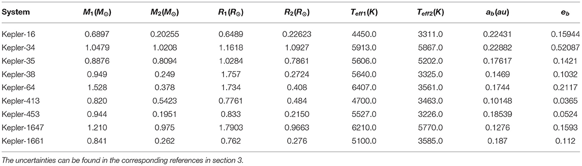
Table 1. Mean physical parameters and orbital elements for the Kepler-16(AB), Kepler-34(AB), Kepler-35(AB), Kepler-38(AB), Kepler-64(AB), Kepler-413(AB), Kepler-453(AB), Kepler-1647(AB), and Kepler-1661(AB) stellar binaries.

TABLE 2

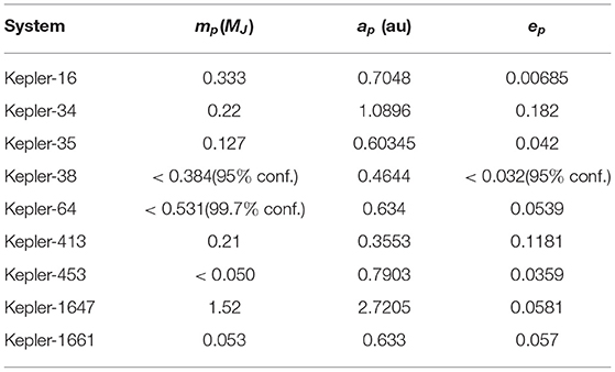
Table 2. Mean mass, semi-major axis, and eccentricity for Kepler-16b, Kepler-34b, Kepler-35b, Kepler-38b, Kepler-64b, Kepler-413b, Kepler-453b, Kepler-1647b, and Kepler-1661b. The uncertainties can be found in the corresponding references in section 3.

First, we calculate all dynamically informed habitable zones assuming no giant planets are present in the systems. That provides us with a first idea of the location of the habitable zones and how the presence of the second star affects the location and extent of the various habitable zones. Then we include the existing giant planet in our model and examine its effect on the habitability of an additional hypothetical terrestrial planet. In both stages, we allowed the eccentricities of the binary and the existing planet to vary. That way we get a better picture of the effect of orbital eccentricity, an important quantity that regulates distances between bodies, on the extent of habitable zones in the system. In order to simplify the complex dynamics in the presence of the giant planet, we acknowledge the double hierarchical structure of the problem that allows us to consider the binary as one massive body located at the barycenter. The two stars at their barycenter are considered as one body of mass m_b = m₁ + m₂, therefore reducing the four-body problem to a three-body one. To describe the dynamical evolution of such a system we made use of the relevant equations in Georgakarakos and Eggl (2015) when a_gp < a_p and Eggl et al. (2012) and Georgakarakos (2003, 2005) when a_gp > a_p, where a_gp is the semi-major axis of the orbit of the giant planet. The stability of that particular kind of triple system was assessed using the criterion developed in Petrovich (2015). The corresponding empirical formula is based on numerical simulations of a star and two planets. The planet-star mass ratios investigated in Petrovich (2015) ranged from 10⁻⁴ to 10⁻², the ratio of the planetary semi-major axes was in the interval [3, 10], while the planetary eccentricities took values in the interval [0, 0.9].

A terrestrial planet on an initially circular orbit in a star-planet-planet system is stable against either ejections or collisions with the central object when

$\begin{array}{ll}\frac{a_p}{a_{gp}(1+e_{gp})}>2.4{\left(\frac{m_{gp}}{m_1+m_2}\right)}^{1/3}{\left(\frac{a_p}{a_{gp}}\right)}^{1/2}.& (20)\end{array}$

Here, m_gp is the mass of the giant planet and e_gp its orbital eccentricity. The above expression is valid when the giant planet is closer to the binary than the terrestrial planet. If the giant planet orbits externally to the terrestrial planet, then the criterion becomes

$\begin{array}{ll}\frac{a_{gp}(1-e_{gp})}{a_p}>2.4{\left(\frac{m_{gp}}{m_1+m_2}\right)}^{1/3}{\left(\frac{a_{gp}}{a_p}\right)}^{1/2}.& (21)\end{array}$

Strictly speaking, the planetary systems investigated here do not fall in the planet-star mass ratios investigated in Petrovich (2015). The planet to planet mass ratio, however, remains within those limits which is ultimately more important for the validity of the stability criterion at hand. This hypothesis can be supported by the reasonable agreement between the stability estimates given by Equations (20) and (21) and those in Georgakarakos (2013), where hierarchical triple systems with a wide range of masses and on initially circular orbits where integrated numerically and their stability limit was determined.

We now proceed to calculating habitable zones for the aforementioned Kepler systems. In a first step, we ignore the presence of residing giant planets in the respective systems. Considering a potential terrestrial planet orbiting the stellar binary, we can determine the borders of the classical and dynamically informed habitable zones for all the Kepler systems under investigation. As we can see from the left column plots of Figures 3–5, all systems but one have well-defined habitable zones and would be capable of hosting a broad range of potentially habitable worlds. The only exception to that is Kepler-16, where more than half of the habitable zone is truncated due to dynamical instability arising from the gravitational perturbations of the stellar binary. A terrestrial planet could only survive near the outer border of the habitable zone with the additional requirement that it does not have a low climate inertia since the PHZ has been completely eliminated.

FIGURE 3

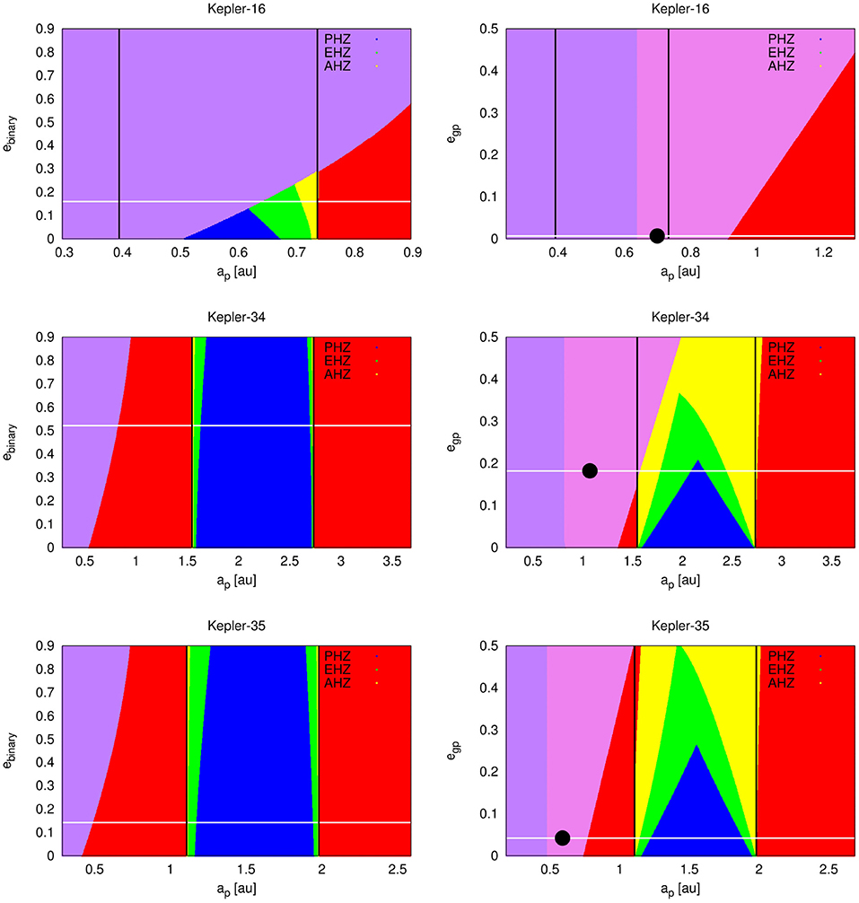
Figure 3. Dynamically informed habitable zones for the Kepler-16, Kepler-34, and Kepler-35 systems. Plots in the left column show the different types of habitable zones without the presence of the known giant planets. The right column includes the influence of the known giant planets. Red colored regions correspond to uninhabitable areas, blue, green, yellow, and purple colors denote the PHZ, the EHZ, the AHZ, and unstable areas according to Holman and Wiegert (1999) stability criterion, respectively. Violet colored areas mark regions of dynamical instability caused by the giant planet in the system (Petrovich, 2015 dynamical stability criterion). The vertical black lines denote the classical habitable zone limits, while the horizontal white line in the left column plots marks the current eccentricity of the binary star orbit. In the right column graphs, the white line marks the current eccentricity of the giant planet orbit. Finally, the black dot in the right column plots shows the position of the giant planet in the presented parameter space.

FIGURE 4

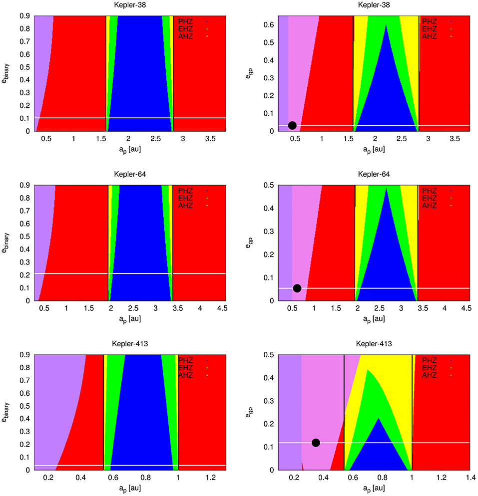
Figure 4. Same as Figure 3 for Kepler-38, Kepler-64, and Kepler-413.

FIGURE 5

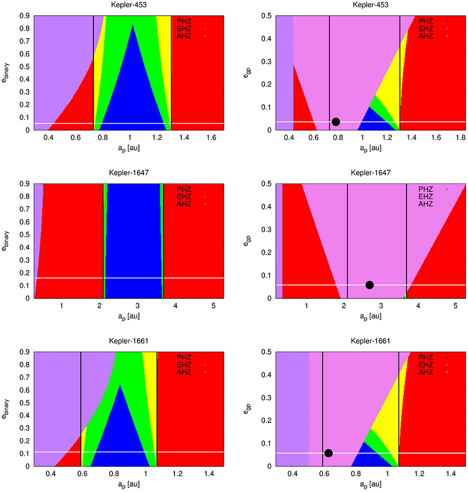
Figure 5. Same as Figure 3 for Kepler-453, Kepler-1647, and Kepler-1661.

When we add the giant planet in our model (right column plots of Figures 3–5), we notice that in Kepler-16 and Kepler-1647 the added gravitational effect of the giant planet renders the entire habitable zone dynamically unstable. Regarding Kepler-16, this is in agreement with other studies such as Quarles et al. (2012); Liu et al. (2013). Note that these results do not exclude the presence of potentially habitable moons around Kepler-16b. In the Kepler-1647 system, the giant planet is located near the middle of the habitable zone. Although Kepler-453b and Kepler-1661b are located inside the classical habitable zones like the other two giant planets mentioned above, they allow a terrestrial planet to exist near the outer border of the habitable zone and they may even allow that planet to have a partial PHZ. This is because of the relatively small masses (Neptune mass) and eccentricities of those planets. In contrast, Kepler-1647b is 1.5M_J and resides near the center of the habitable zone.

Regarding the remaining systems, the entire classical habitable zone is essentially dynamically stable. The difference between dynamically informed habitable zones with and without the giant planet perturbers shows, however, that the influence of giant planets goes beyond dynamical instability. In Kepler-34, potentially habitable worlds with low climate inertia could only remain habitable in a tiny region centered around 2.17 au. This can be seen from a comparison between the extent of the PHZ and the black vertical lines in the middle row right panel of Figure 3. Relatively dry planets with a low concentration of greenhouse gases would fall into this category. On the other hand, Kepler-35, Kepler-38, and Kepler-64 could host potentially habitable worlds with low climate inertia over a significant fraction (more than 75%) of their classical habitable zone (Figures 4, 5). Finally, the extent of the PHZ of Kepler-413 is around 40% of its classical habitable zone. While not prohibitive, the presence of giant planets in Kepler-34, Kepler-413, Kepler-453, and Kepler-1661 requires additional terrestrial worlds to buffer significant variations in irradiation in order to remain habitable.

For comparison, some results from Haghighipour and Kaltenegger (2013), Cuntz (2014), Cuntz (2015), and Wang and Cuntz (2019) are also provided. Our results seem to be in good agreement with those of Cuntz (2014, 2015) and Wang and Cuntz (2019), with our classical habitable zone being a bit wider. In order to compare with Haghighipour and Kaltenegger (2013), we use Kopparapu et al. (2013) to calculate our classical habitable zone as that specific climate model was used by Haghighipour and Kaltenegger (2013) for their habitable zone calculations. In this case, however, it is more difficult to make a direct comparison as Haghighipour and Kaltenegger (2013) used time variable habitable zones centered at the primary star. Habitable zones borders for the Kepler systems under investigation are presented in Table 3.

TABLE 3

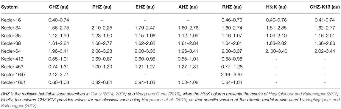
Table 3. Habitable zone limits for Kepler-16, Kepler-34, Kepler-35, Kepler-38, Kepler-64, Kepler-413, Kepler-453, Kepler-1647, and Kepler-1661.

4. Discussion and summary

We present an analytical approach to determine dynamically informed habitable zones in binary star systems with a circumbinary giant planet. The method takes into consideration the orbital evolution of the giant and terrestrial planet as well as different responses of planetary climates to variations in the quantity and spectral energy distribution of incoming radiation. It does not apply, however, during the planet formation stage, when we can have planets migrating due to interactions with the protoplanetary disk or planet-planet scattering events during late stage formation. In addition, we do not consider systems where there is significant tidal interaction between the two stars which may lead to changes in the orbit and rotation rates of the stars, as well as to changes in the emission of XUV radiation that can affect the atmosphere of a planet within the habitable zone (e.g., Sanz-Forcada et al., 2014; Johnstone et al., 2019).

As the method mainly relies on analytical equations, it can provide a quick assessment of the capability of terrestrial circumbinary planets in complex dynamical environments to retain liquid water on their surface. The construction and comparison of dynamically informed habitable zones, i.e., the PHZ, the EHZ and the AHZ allows us to better understand where potentially habitable worlds with different climate characteristics can exist in binary star systems. The method presented here is very versatile as it has been constructed in such a way that it does not depend on the dynamical model and the insolation limits.

In this work, we investigated the effects of stellar binarity and circumbinary giant planets on the habitable zones of nine systems observed by the Kepler mission. We confirm earlier studies that suggest Kepler-16 is not suitable for hosting a terrestrial planet within its classical habitable zone. The situation is similar for Kepler-1647. In contrast, Kepler-34, Kepler-35, Kepler-38, Kepler-64, and Kepler-413 seemed more promising with Kepler-38 being the best candidate in this respect. Kepler-453 and Kepler-1661 stand between the previous two categories of systems. We find that nearly equal binary mass ratios and small eccentricities of the perturbing bodies provide favorable, from the orbital evolution point of view, conditions for an Earth-like planet to exist in the habitable zone. We show, furthermore, that the presence of a giant planet can have a significant effect on the potential habitability of terrestrial worlds in the same system. We, thus, recommend gravitational perturbations of known giant planets to be taken into account in future studies regarding habitability in binary star systems.

Data Availability Statement

The original contributions presented in the study are included in the article/supplementary material, further inquiries can be directed to the corresponding author/s.

Author Contributions

NG and SE: conceptualization, methodology, investigation, resources, and writing–original draft preparation-revised version. NG: software and data curation. NG, SE, and ID-D: validation. All authors have read and agreed to the published version of the manuscript.

Conflict of Interest

The authors declare that the research was conducted in the absence of any commercial or financial relationships that could be construed as a potential conflict of interest.

Acknowledgments

SE acknowledges support from the DIRAC Institute in the Department of Astronomy at the University of Washington. The DIRAC Institute is supported through generous gifts from the Charles and Lisa Simonyi Fund for Arts and Sciences, and the Washington Research Foundation. The results reported herein benefited from collaborations and/or information exchange within NASA's Nexus for Exoplanet System Science (NExSS) research coordination network sponsored by NASA's Science Mission Directorate. This research has made use of the NASA Exoplanet Archive, which is operated by the California Institute of Technology, under contract with the National Aeronautics and Space Administration under the Exoplanet Exploration Program.

Footnotes

1. ^https://exoplanetarchive.ipac.caltech.edu/

References

Cukier, W., Kopparapu, R. K., Kane, S. R., Welsh, W., Wolf, E., Kostov, V., et al. (2019). Habitable zone boundaries for circumbinary planets. Publ. Astron. Soc. Pac. 131:124402. doi: 10.1088/1538-3873/ab50cb

PubMed Abstract | CrossRef Full Text | Google Scholar

Cuntz, M. (2014). S-type and P-type habitability in stellar binary systems: a comprehensive approach. I. Method and applications. Astrophys. J. 780:14. doi: 10.1088/0004-637X/780/1/14

CrossRef Full Text | Google Scholar

Cuntz, M. (2015). S-type and P-type habitability in stellar binary systems: a comprehensive approach. II. Elliptical orbits. Astrophys. J. 798:101. doi: 10.1088/0004-637X/798/2/101

CrossRef Full Text | Google Scholar

Doyle, L. R., Carter, J. A., Fabrycky, D. C., Slawson, R. W., Howell, S. B., Winn, J. N., et al. (2011). Kepler-16: a transiting circumbinary planet. Science 333:1602. doi: 10.1126/science.1210923

CrossRef Full Text | Google Scholar

Eggl, S. (2018). “Habitability of Planets in Binary Star Systems,” in Handbook of Exoplanets, eds H. J. Deeg and J. A. Belmonte (Springer International Publishing), 61.

Google Scholar

Eggl, S., Georgakarakos, N., and Pilat-Lohinger, E. (2020). Habitable zones in binary star systems: a zoology. Galaxies 8:65. doi: 10.3390/galaxies8030065

CrossRef Full Text | Google Scholar

Eggl, S., Pilat-Lohinger, E., Georgakarakos, N., Gyergyovits, M., and Funk, B. (2012). An analytic method to determine habitable zones for S-type planetary orbits in binary star systems. Astrophys. J. 752:74. doi: 10.1088/0004-637X/752/1/74

CrossRef Full Text | Google Scholar

Forgan, D. (2014). Assessing circumbinary habitable zones using latitudinal energy balance modelling. Mon. Not. R. Astron. Soc. 437, 1352–1361. doi: 10.1093/mnras/stt1964

CrossRef Full Text | Google Scholar

Georgakarakos, N. (2003). Eccentricity evolution in hierarchical triple systems with eccentric outer binaries. Mon. Not. R. Astron. Soc. 345, 340–348. doi: 10.1046/j.1365-8711.2003.06942.x

CrossRef Full Text | Google Scholar

Georgakarakos, N. (2005). Erratum: eccentricity evolution in hierarchical triple systems with eccentric outer binaries. Mon. Not. R. Astron. Soc. 362:748. doi: 10.1111/j.1365-2966.2005.09441.x

CrossRef Full Text | Google Scholar

Georgakarakos, N. (2008). Stability criteria for hierarchical triple systems. Celest. Mech. Dynam. Astron. 100, 151–168. doi: 10.1007/s10569-007-9109-2

CrossRef Full Text | Google Scholar

Georgakarakos, N. (2009). Improved equations for eccentricity generation in hierarchical triple systems. Mon. Not. R. Astron. Soc. 392, 1253–1263. doi: 10.1111/j.1365-2966.2008.14143.x

CrossRef Full Text | Google Scholar

Georgakarakos, N. (2013). The dependence of the stability of hierarchical triple systems on the orbital inclination. New Astron. 23, 41–48. doi: 10.1016/j.newast.2013.02.004

CrossRef Full Text | Google Scholar

Georgakarakos, N., and Eggl, S. (2015). Analytic orbit propagation for transiting circumbinary planets. Astrophys. J. 802:94. doi: 10.1088/0004-637X/802/2/94

CrossRef Full Text | Google Scholar

Georgakarakos, N., Eggl, S., and Dobbs-Dixon, I. (2018). Giant planets: good neighbors for habitable worlds? Astrophys. J. 856:155. doi: 10.3847/1538-4357/aaaf72

CrossRef Full Text | Google Scholar

Gilbert, E. A., Barclay, T., Schlieder, J. E., Quintana, E. V., Hord, B. J., Kostov, V. B., et al. (2020). The First Habitable-zone Earth-sized Planet from TESS. I. Validation of the TOI-700 System. Astron. J. 160:116. doi: 10.3847/1538-3881/aba4b2

CrossRef Full Text | Google Scholar

Gillon, M., Jehin, E., Lederer, S. M., Delrez, L., de Wit, J., Burdanov, A., et al. (2016). Temperate Earth-sized planets transiting a nearby ultracool dwarf star. Nature 533, 221–224. doi: 10.1038/nature17448

PubMed Abstract | CrossRef Full Text | Google Scholar

Haghighipour, N., and Kaltenegger, L. (2013). Calculating the habitable zone of binary star systems. II. P-type binaries. Astrophys. J. 777:166. doi: 10.1088/0004-637X/777/2/166

CrossRef Full Text | Google Scholar

Haqq-Misra, J., Wolf, E. T., Welsh, W. F., Kopparapu, R. K., Kostov, V., and Kane, S. R. (2019). Constraining the magnitude of climate extremes from time-varying instellation on a circumbinary terrestrial planet. J. Geophys. Res. 124, 3231–3243. doi: 10.1029/2019JE006222

CrossRef Full Text | Google Scholar

Holman, M. J., and Wiegert, P. A. (1999). Long-term stability of planets in binary systems. Astron. J. 117, 621–628. doi: 10.1086/300695

CrossRef Full Text | Google Scholar

Jaime, L. G., Aguilar, L., and Pichardo, B. (2014). Habitable zones with stable orbits for planets around binary systems. Mon. Not. R. Astron. Soc. 443, 260–274. doi: 10.1093/mnras/stu1052

CrossRef Full Text | Google Scholar

Johnstone, C. P., Pilat-Lohinger, E., Lüftinger, T., Güdel, M., and Stökl, A. (2019). Stellar activity and planetary atmosphere evolution in tight binary star systems. Astron. Astrophys. 626:A22. doi: 10.1051/0004-6361/201832805

CrossRef Full Text | Google Scholar

Kane, S. R., and Hinkel, N. R. (2013). On the habitable zones of circumbinary planetary systems. Astrophys. J. 762:7. doi: 10.1088/0004-637X/762/1/7

CrossRef Full Text | Google Scholar

Kasting, J. F., Whitmire, D. P., and Reynolds, R. T. (1993). Habitable zones around main sequence stars. Icarus 101, 108–128. doi: 10.1006/icar.1993.1010

PubMed Abstract | CrossRef Full Text | Google Scholar

Kopparapu, R. K., Ramirez, R., Kasting, J. F., Eymet, V., Robinson, T. D., Mahadevan, S., et al. (2013). Erratum: “habitable zones around main-sequence stars: new estimates” (2013, ApJ, 765, 131) </A>. Astrophys. J. 770:82. doi: 10.1088/0004-637X/770/1/82

CrossRef Full Text | Google Scholar

Kopparapu, R. K., Ramirez, R. M., SchottelKotte, J., Kasting, J. F., Domagal-Goldman, S., and Eymet, V. (2014). Habitable zones around main-sequence stars: dependence on planetary mass. Astrophys. J. Lett. 787:L29. doi: 10.1088/2041-8205/787/2/L29

CrossRef Full Text | Google Scholar

Kostov, V. B., McCullough, P. R., Carter, J. A., Deleuil, M., Díaz, R. F., Fabrycky, D. C., et al. (2014). Kepler-413b: a slightly misaligned, neptune-size transiting circumbinary planet. Astrophys. J. 784:14. doi: 10.1088/0004-637X/784/1/14

CrossRef Full Text | Google Scholar

Kostov, V. B., Orosz, J. A., Welsh, W. F., Doyle, L. R., Fabrycky, D. C., Haghighipour, N., et al. (2016). Kepler-1647b: the largest and longest-period kepler transiting circumbinary planet. Astrophys. J. 827:86. doi: 10.3847/0004-637X/827/1/86

CrossRef Full Text | Google Scholar

Liu, H.-G., Zhang, H., and Zhou, J.-L. (2013). Where to find habitable “Earths” in circumbinary systems. Astrophys. J. Lett. 767:L38. doi: 10.1088/2041-8205/767/2/L38

CrossRef Full Text | Google Scholar

Marzari, F., and Thebault, P. (2019). Planets in binaries: formation and dynamical evolution. Galaxies 7:84. doi: 10.3390/galaxies7040084

CrossRef Full Text | Google Scholar

Orosz, J. A., Welsh, W. F., Carter, J. A., Brugamyer, E., Buchhave, L. A., Cochran, W. D., et al. (2012). The neptune-sized circumbinary planet Kepler-38b. Astrophys. J. 758:87. doi: 10.1088/0004-637X/758/2/87

CrossRef Full Text | Google Scholar

Orosz, J. A., Welsh, W. F., Haghighipour, N., Quarles, B., Short, D. R., Mills, S. M., et al. (2019). Discovery of a third transiting planet in the Kepler-47 circumbinary system. Astron. J. 157:174. doi: 10.3847/1538-3881/ab0ca0

CrossRef Full Text | Google Scholar

Petrovich, C. (2015). The stability and fates of hierarchical two-planet systems. Astrophys. J. 808:120. doi: 10.1088/0004-637X/808/2/120

CrossRef Full Text | Google Scholar

Popp, M., and Eggl, S. (2017). Climate variations on Earth-like circumbinary planets. Nat. Commun. 8:14957. doi: 10.1038/ncomms14957

PubMed Abstract | CrossRef Full Text | Google Scholar

Quarles, B., Musielak, Z. E., and Cuntz, M. (2012). Habitability of Earth-mass planets and moons in the Kepler-16 system. Astrophys. J. 750:14. doi: 10.1088/0004-637X/750/1/14

CrossRef Full Text | Google Scholar

Rodriguez, J. E., Vanderburg, A., Zieba, S., Kreidberg, L., Morley, C. V., Eastman, J. D., et al. (2020). The first habitable-zone Earth-sized planet from TESS. II. Spitzer confirms TOI-700 d. Astron. J. 160:117. doi: 10.3847/1538-3881/aba4b3

CrossRef Full Text | Google Scholar

Sanz-Forcada, J., Desidera, S., and Micela, G. (2014). Effects of X-ray and extreme UV radiation on circumbinary planets. Astron. Astrophys. 570:A50. doi: 10.1051/0004-6361/201323231

CrossRef Full Text | Google Scholar

Schwamb, M. E., Orosz, J. A., Carter, J. A., Welsh, W. F., Fischer, D. A., Torres, G., et al. (2013). Planet hunters: a transiting circumbinary planet in a quadruple star system. Astrophys. J. 768:127. doi: 10.1088/0004-637X/768/2/127

CrossRef Full Text | Google Scholar

Shevchenko, I. I., Melnikov, A. V., Popova, E. A., Bobylev, V. V., and Karelin, G. M. (2019). Circumbinary planetary systems in the solar neighborhood: stability and habitability. Astron. Lett. 45, 620–626. doi: 10.1134/S1063773719080097

CrossRef Full Text | Google Scholar

Socia, Q. J., Welsh, W. F., Orosz, J. A., Cochran, W. D., Endl, M., Quarles, B., et al. (2020). Kepler-1661 b: a neptune-sized kepler transiting circumbinary planet around a grazing eclipsing binary. Astron. J. 159:94. doi: 10.3847/1538-3881/ab665b

CrossRef Full Text | Google Scholar

Wang, Z., and Cuntz, M. (2019). S-type and P-type habitability in stellar binary systems: a comprehensive approach. III. Results for Mars, Earth, and Super-Earth Planets. Astrophys. J. 873:113. doi: 10.3847/1538-4357/ab0377

CrossRef Full Text | Google Scholar

Way, M. J., and Georgakarakos, N. (2017). Effects of variable eccentricity on the climate of an Earth-like world. Astrophys. J. Lett. 835:L1. doi: 10.3847/2041-8213/835/1/L1

CrossRef Full Text | Google Scholar

Welsh, W. F., Orosz, J. A., Carter, J. A., Fabrycky, D. C., Ford, E. B., Lissauer, J. J., et al. (2012). Transiting circumbinary planets Kepler-34 b and Kepler-35 b. Nature 481, 475–479. doi: 10.1038/nature10768

PubMed Abstract | CrossRef Full Text | Google Scholar

Welsh, W. F., Orosz, J. A., Short, D. R., Cochran, W. D., Endl, M., Brugamyer, E., et al. (2015). Kepler 453 b - The 10th kepler transiting circumbinary planet. Astrophys. J. 809:26. doi: 10.1088/0004-637X/809/1/26

CrossRef Full Text | Google Scholar

Wolf, E. T., Haqq-Misra, J., Kopparapu, R., Fauchez, T. J., Welsh, W. F., Kane, S. R., et al. (2020). The resilience of habitable climates around circumbinary stars. J. Geophys. Res. 125:e06576. doi: 10.1029/2020JE006576

CrossRef Full Text | Google Scholar

Yadavalli, S. K., Quarles, B., Li, G., and Haghighipour, N. (2020). Effects of flux variation on the surface temperatures of Earth-analog circumbinary planets. Mon. Not. R. Astron. Soc. 499, 1506–1521. doi: 10.1093/mnras/staa2980

CrossRef Full Text | Google Scholar

Appendix

Planetary Eccentricity Equations

We follow Georgakarakos and Eggl (2015) to calculate the maximum orbital eccentricity $e_p^{max}$ and average squared eccentricity $\langle e_p^2\rangle$ for a circumbinary planet:

$\begin{array}{l}{e}_p^{max}=\frac{m_1{m}_2}{{(m_1+m_2)}^{\frac{4}{3}}{M}^{\frac{2}{3}}}\frac{1}{X^{\frac{4}{3}}}\\ \left[\frac{3}{2}+\frac{17}{2}{e}_b^2+\frac{1}{X}\left(3+19e_b+\frac{21}{8}{e}_b^2-\frac{3}{2}{e}_b^3\right)\right]\\ \begin{array}{l}+2\left|\frac{K_2}{K_1-K_3}\right|\end{array}& (22)\end{array}$

and

$\begin{array}{l}\langle e_p^2\rangle =\frac{m_1^2{m}_2^2}{{(m_1+m_2)}^{\frac{8}{3}}{M}^{\frac{4}{3}}}\frac{1}{X^{\frac{8}{3}}}[\frac{9}{8}+\frac{27}{8}{e}_b^2+\frac{887}{64}{e}_b^4\\ -\frac{975}{64}\frac{1}{X}{e}_b^4\sqrt{1-e_b^2}++\frac{1}{X^2}(\frac{225}{64}+\frac{6619}{64}{e}_b^2-\frac{26309}{512}{e}_b^4\\ -\frac{393}{64}{e}_b^6)]+2{(\frac{K_2}{K_1-K_3})}^2,& (23)\end{array}$

where

$\begin{array}{ll}M=m_1+m_2+m_p& (24)\end{array}$

$\begin{array}{ll}X=\sqrt{\frac{m_1+m_2}{M}}{\left(\frac{a_p}{a_b}\right)}^{\frac{3}{2}}& (25)\end{array}$

$\begin{array}{ll}{K}_1=\frac{3}{8}\frac{\sqrt{{G}M}{m}_1{m}_2{a}_b^2}{{(m_1+m_2)}^2{a}_p^{\frac{7}{2}}}(2+3e_b^2)& (26)\end{array}$

$\begin{array}{ll}{K}_2=\frac{15}{64}\frac{\sqrt{{G}M}{m}_1{m}_2(m_1-m_2)a_b^3}{{(m_1+m_2)}^3{a}_p^{\frac{9}{2}}}{e}_b(4+3e_b^2)& (27)\end{array}$

$\begin{array}{ll}{K}_3=\frac{3}{4}\frac{\sqrt{{G}}{m}_p{a}_b^{\frac{3}{2}}\sqrt{1-e_b^2}}{{(m_1+m_2)}^{\frac{1}{2}}{a}_p^3},& (28)\end{array}$

and ${G}$ is the gravitational constant.

Equations (22) and (23) were also used when we added the giant planet to our model and the orbit of the giant planet was interior to that of the terrestrial planet. In order to use the above equations in that respect, we replace m₁ with m_b = m₁ + m₂, m₂ with m_gp, a_b with a_gp, e_b with e_gp and M = m_b + m_gp + m_p.

When the orbit of the giant planet was exterior to that of the terrestrial planet, we used the below equations from Eggl et al. (2012) and Georgakarakos (2003, 2005) (with the notation of this work):

$\begin{array}{l}{e}_p^{max}=\frac{m_{gp}}{M{X}^{5/3}}[\frac{15}{64}\frac{m_1-m_p}{{(m_1+m_p)}^{2/3}{M}^{1/3}}\frac{(4+11e_{gp}^2)}{{(1-e_{gp}^2)}^{5/2}}+\frac{3}{4}+\\ +\frac{11}{4}\frac{1}{X^{1/3}}\frac{{(1+e_{gp})}^3}{{(1-e_{gp}^2)}^3}\frac{1}{X^{4/3}}\frac{{(1+e_{gp})}^4(6+11e_{gp})}{{(1-e_{gp}^2)}^{9/2}}]\\ +2\frac{C}{B-A},& (29)\end{array}$

and

$\begin{array}{l}\langle e_p^2\rangle =\frac{m_{gp}^2}{M^2}\frac{1}{X^4{(1-e_{gp}^2)}^{\frac{9}{2}}}\{\frac{43}{8}+\frac{129}{8}{e}_{gp}^2+\frac{129}{64}{e}_{gp}^4\\ +\frac{1}{{(1-e_{gp}^2)}^{\frac{3}{2}}}\left(\frac{43}{8}+\frac{645}{16}{e}_{gp}^2+\frac{1935}{64}{e}_{gp}^4++\frac{215}{128}{e}_{gp}^6\right)\\ +\frac{1}{X^2{(1-e_{gp}^2)}^3}[\frac{365}{18}+\frac{44327}{144}{e}_{gp}^2+\frac{119435}{192}{e}_{gp}^4\\ +\frac{256105}{1152}{e}_{gp}^6+\frac{68335}{9216}{e}_{gp}^8++\frac{1}{{(1-e_{gp}^2)}^{\frac{3}{2}}}(\frac{365}{18}+\\ \frac{7683}{16}{e}_{gp}^2+\frac{28231}{16}{e}_{gp}^4+\frac{295715}{192}{e}_{gp}^6+\frac{2415}{8}{e}_{gp}^8\\ +\frac{12901}{2048}{e}_{gp}^{10})]++\frac{1}{X{(1-e_{gp}^2)}^{\frac{3}{2}}}[\frac{61}{3}+\frac{305}{2}{e}_{gp}^2\\ +\frac{915}{8}{e}_{gp}^4+\frac{305}{48}{e}_{gp}^6+\frac{1}{{(1-e_{gp}^2)}^{\frac{3}{2}}}(\frac{61}{3}+\frac{854}{3}{e}_{gp}^2+\\ +\frac{2135}{4}{e}_{gp}^4+\frac{2135}{12}{e}_{gp}^6+\frac{2135}{384}{e}_{gp}^8)]+m_{*}^2{X}^{\frac{2}{3}}(1-e_{gp}^2)\\ [\frac{225}{256}+\frac{3375}{1024}{e}_{gp}^2+\frac{7625}{2048}{e}_{gp}^4+\\ +\frac{29225}{8192}{e}_{gp}^6+\frac{48425}{16384}{e}_{gp}^8+\frac{825}{2048}{e}_{gp}^{10}+\frac{1}{{(1-e_{gp}^2)}^{\frac{3}{2}}}\\ \left(\frac{225}{256}+\frac{2925}{1024}{e}_{gp}^2+\frac{775}{256}{e}_{gp}^4++\frac{2225}{8192}{e}_{gp}^6+\frac{25}{512}{e}_{gp}^8\right)]\\ +m_{*}^2\frac{1}{X^{\frac{4}{3}}{(1-e_{gp}^2)}^2}[\frac{8361}{4096}+\frac{125415}{8192}{e}_{gp}^2+\frac{376245}{32768}{e}_{gp}^4+\\ +\frac{41805}{65536}{e}_{gp}^6+\frac{1}{{(1-e_{gp}^2)}^{\frac{3}{2}}}(\frac{8361}{4096}+\frac{58527}{2048}{e}_{gp}^2\\ +\frac{877905}{16384}{e}_{gp}^4+\frac{292635}{16384}{e}_{gp}^6\\ +\frac{292635}{524288}{e}_{gp}^8)]\}+2{(\frac{C}{B-A})}^2,& (30)\end{array}$

where

$\begin{array}{ll}M=m_b+m_p+m_{gp}& (31)\end{array}$

$\begin{array}{ll}{m}_{*}=\frac{m_p-m_b}{{(m_b+m_p)}^{2/3}{M}^{1/3}}& (32)\end{array}$

$\begin{array}{ll}X=\sqrt{\frac{m_b+m_p}{M}}{\left(\frac{a_{gp}}{a_p}\right)}^{\frac{3}{2}}& (33)\end{array}$

$\begin{array}{ll}C=\frac{5}{4}\frac{(m_b-m_p)e_{gp}{a}_p}{(m_b+m_p){(1-e_{gp}^2)}^{5/2}{a}_{gp}}& (34)\end{array}$

$\begin{array}{ll}B=\frac{1}{{(1-e_{gp}^2)}^{3/2}}& (35)\end{array}$

$\begin{array}{ll}A=\frac{m_b{m}_p{M}^{1/2}}{m_{gp}{(m_b+m_p)}^{3/2}}\frac{1}{{(1-e_{gp})}^2}{\left(\frac{a_p}{a_{gp}}\right)}^{1/2}.& (36)\end{array}$

The above equations can be used for nearly coplanar systems and systems that are not close to mean motion resonances. Also, the equations become less reliable as the maximum planetary eccentricity gets larger than 0.2–0.25.