Geoeffectiveness Prediction of CMEs

1 Introduction

Forecasting if a coronal mass ejection (CME) is geoeffective (i.e., capable of causing a geomagnetic disturbance) is a subject of increasing interest during the last decade, because of the high impact these eruptive events may have on the technological system in orbit or on Earth. Each model must take into consideration some approximation and, thus, no model can currently predict with a 100% accuracy the impact of a CME.

1.1 Geoeffectiveness of CMEs

It is known that the CMEs reaching Earth’s magnetosphere can produce large perturbations in the geomagnetic field known as geomagnetic storms. The first indication of a geomagnetic storm is shown by a decrease of the Dst index, with storms being classified as small if −50 nT $<$ Dst $\mathrm{⩽}$ −30 nT, moderate (−50 nT $\mathrm{⩾}$ Dst $>$ −100 nT), and intense (Dst $\mathrm{⩽}$ −100 nT) (Gonzalez et al., 1994).

The geoeffective CMEs predominantly originate from sources near the central meridian, mostly from the western hemisphere (Srivastava and Venkatakrishnan, 2004; Zhang et al., 2007). The most geoeffective tend to be the energetic frontside halo CMEs, which are associated with strong soft X-ray flares (Gopalswamy et al., 2007).

The geoeffectiveness of the CME will also depend on its particular evolution, which is related to both internal CME properties (kinematic, geometric and magnetic), and (external) solar wind plasma properties (see e.g., the review by Manchester et al., 2017).

It was shown that interacting CMEs in the heliosphere amplify the geomagnetic response (Scolini et al., 2020). This amplification could be due to shock compression inside interplanetary CMEs (ICMEs) (see e.g., Shen et al., 2018; Xu et al., 2019), due to the generation of high energy protons (see e.g., Joshi et al., 2013) or due to the heights above the photosphere at which the shocks are formed (see e.g., Gopalswamy et al., 2013).

1.2 Solar Cycle Dependence

Correlations between CMEs, ICMEs and the sunspot number have been intensively studied (Gopalswamy et al., 2010; Webb and Howard, 2012; Lamy et al., 2019) to conclude that the CME rate usually follows the solar activity indices (Möstl et al., 2020). Chi et al. (2016) confirmed that the yearly ICME rate follows the sunspot number. This implies that during maximum of solar activity more CMEs arrive at Earth compared with the minimum solar activity period.

Comparing the last two solar cycles, the 23rd one has been more geoeffective than the 24th one (Bhatt and Chandra, 2020). Solar cycle 24 was characterized by low flare activity and the main contribution to geoeffective events was made by CMEs (Bruevich and Yakunina, 2020).

The present study covers the solar cycle 24 and it takes into consideration the possibility that there is a model simple enough, based only on CME parameters derived close to the Sun, which could predict that a CME will reach the Earth and it will produce a geomagnetic storm.

The model is based on an updated logistic regression method (Srivastava, 2005; Besliu-Ionescu et al., 2019), that attempts to forecast if a CME will arrive at the Earth and if it will trigger a geomagnetic storm. The model is run for a selection of CMEs listed in the LASCO catalogue (Yashiro et al., 2004) from January 2008 to May 2020.

The model takes into consideration the full-chain of events CMEs-ICMEs-Geomagnetic Storms and outputs the probability of a CME being geoeffective or not.

The paper is structured as follows: Section 2 presents the method used in this study, Section 3 describes the results of the non-linear logistic regression model, Section 4 discusses the main findings of this study and proposes future research.

2 Nonlinear Logistic Regression

2.1 Data Selection

In order to select our events we looked in the LASCO CME catalogue (https://cdaw.gsfc.nasa.gov/CME_list/) in the period between January 2008 and May 2020.

In this period there were approximately 17,000 CMEs detected. We excluded CMEs catalogued with “poor events” and “very poor events,” which amounted to more than 12,500 CMEs, i.e., about 73% of the total CMEs observed by LASCO in the studied period. The classification of events is linked to the quality index (0–5) for the tracking feature (leading edge) of each CME: very poor, poor, fair, typical, good, and excellent. Very poor event (quality index 0) means a CME with an ill-defined leading edge and poor event (quality index 1) is a CME where the leading edge is not clear and sharp enough to be accurately tracked in different frames (see e.g., Yashiro et al., 2004). The poor events were excluded in order to have a consistent list where one can measure with accuracy different characteristics of the CMEs (speed, angular width, etc.). This selection criteria left us with a database of 4,576 CMEs.

We further excluded the CMEs that have an angular width smaller than 60°, leaving us with 2,794 CMEs to study. This second selection criteria is justified since, in order for a CME to arrive at the Earth and to produce a geomagnetic storm it should have a large angular extent (e.g., Schwenn, 2006; Zhang et al., 2007).

In general, full halo (apparent angular width of 360°) and partial halo (apparent angular width larger than 120°) CMEs in LASCO images are considered as potential candidates to impact the Earth (if their source region is on the Earth-facing solar disk). A normal CME, seen above the limb with an angular width of around 60°, will appear as a halo CME or partial halo CME when oriented along the Sun-Earth-line (both: towards to or away from Earth) or some 40° off that line, respectively (e.g., Schwenn, 2006).

However, it was also demonstrated that narrow CMEs (AW $\mathrm{⩽}$ 20$°$) can arrive at Earth and exhibit clear in-situ signatures (e.g., Kilpua et al., 2014). Still, none of these narrow CMEs that arrived at Earth were detected by LASCO. Many studies consider eruptions below 10$°$ angular width as being jets and not CMEs (e.g., Paraschiv et al., 2010) (review of Raouafi et al., 2016, etc.). The averaged angular width of the CMEs wider than 30$°$ is around 60$°$ (e.g., the review of Webb and Howard, 2012) which also contributed to our selection criteria. We decided to re-include two CMEs that were poor events, but have reached the interplanetary space, such as listed by the ICME catalogue (Richardson and Cane, 2010). Thus, the database for the current study has 2,796 events.

The association of our events with the interplanetary disturbances was extracted from the ICME Catalogue (Richardson and Cane, 2010) which is available online at http://www.srl.caltech.edu/ACE/ASC/DATA/level3/icmetable2.htm. There where 49 CMEs that have reached the Earth during the selected period. CME-ICME association method, described by Cane and Richardson (2003), is based on studying the proton temperature from the solar wind for periods of abnormally low values. Then the ratio of the observed vs. the expected proton temperature is evaluated and the magnetic observations are added. An ICME interval could be inferred from reduced fluctuations and some degree of organization in the magnetic field and will be bounded by distinct magnetic field discontinuities which may be accompanied by abrupt changes in plasma parameters (Cane and Richardson, 2003).

Out of these 49 ICMEs, 16 did not produce any geomagnetic disturbances (i.e., Dst_min was larger than −30 nT), four were associated with minor geomagnetic storms (Dst_min between −30 and −50 nT) and 29 were followed by moderate or intense geomagnetic storms (Dst_min$\mathrm{⩽}$ −50 nT).

The Dst_min is the minimum value of the Dst index recorded during the geomagnetic storm marking the end of its main phase, value which is used when cataloging the intensity of the storm.

The location of the CME on the solar disk was derived by checking each event individually. We looked for signatures like dimmings, waves, eruptive prominences. We looked at the combined EUV (SOHO/EIT or SDO/AIA) and white-light (LASCO) movies as given in the catalogue. If nothing was seen in running difference images, we checked EUV normal movies (for e.g., sdoa193_c2rdf.html in Java Movie) to better see the dimmings and the waves. For dimmings we also checked the Solar Demon catalogue (Kraaikamp and Verbeeck, 2015): http://solardemon.oma.be/science/dimmings.php?days=0&dimming_threshold=0&dimming_location=1&science=1. For erupting prominences we checked the AIA prominence catalogue (Yashiro et al., 2020): https://cdaw.gsfc.nasa.gov/CME_list/autope/.

2.2 Method

Predictive models are used in almost every scientific field. Given a set of independent variables, the output of such a model will compute the probability that the dependant variable will have a certain behavior when the combination of the independent variables is the “right-one.”

The logistic regression is a class of regression that needs an independent variable or a set of independent variables to predict a dependent one. Therefore, besides the five independent variables (CME speed at 20 solar radii, its angular width, measured position angle, the acceleration and a binary variable for position), the model needs a dependent one. For this we have chosen a binary variable defined by 0 if the Dst_min value was $>$ −30 nT (i.e., no geomagnetic storm detected), and 1 for Dst_min$\mathrm{⩽}$ −30 nT (i.e., a storm was identified), identical to the binary one used by Besliu-Ionescu et al. (2019).

The solar wind sometimes completes accelerating before 20 solar radii (Nakagawa et al., 2006). Thus, the speed at 20 solar radii better represents the state of the CME after escaping the solar corona.

The model used in this study is a modified version of Srivastava (2005) and has been applied in Besliu-Ionescu et al. (2019) in a modified version.

The equation used in the model is:

${\mathrm{\Pi }}_i=\frac{1}{1+e^{\left(-Z_i\right)}}(1)$

where $Z_i$ is

$Z_i=b_0+{\displaystyle \sum }_{j=1}^5{b}_j\times x_j(2)$

$\text{Π}$ represents the probability of the occurrence of a geomagnetic storm given the ith observation of the CME. $Z_i$ is a linear function of the observations estimated as a natural logarithm of the odds of the occurrence of the geomagnetic storm (Srivastava, 2005). $x_i$ represents the CME observations (CME speed at 20 solar radii, CME angular width, measured position angle, acceleration and a binary variable for its position).

The initial Srivastava (2005) model used a database of 55 geoeffective events that were defined as full chains CME–ICME–geomagnetic storms (intense and super intense). They used a set of seven independent variables describing the CME: its width, speed, its association with flare and its location; and the interplanetary conditions: the magnetic field intensity, the southern component of the interplanetary magnetic field and the ram pressure. The goal of the model was to predict the occurrence of a geomagnetic storm according to the properties of the selected events, used as independent variables, by defining a binary dependant variable with 0, for intense geomagnetic storms, and 1, for super-intense ones. The dataset was divided in training (46 events) and validation (9) sets and the obtained success rates for that model were 85 and 77.7% for the training, respectively, validation sets.

Besliu-Ionescu et al. (2019) had a slightly different approach than Srivastava (2005) as they used only CME solar parameters and excluded any ICMEs measurements. The parameters (independent variables in the model) used by Besliu-Ionescu et al. (2019) were the measured position angle of the CME, its angular width, linear speed, the acceleration, the latitude and longitude of its source, the association with a flare (binary variable to be 1 for the events where there was a flare associated with the CME, and 0 otherwise), the flare importance index (Maris et al., 2002), the magnetic active region type (a scaled value between 0 and 1 as a function of the magnetic classification of the active region) and the orientation of the neutral line (a number describing the direction of the neutral line – NS, EW, NW-SW and NE-SW). The computed proportions of correctness (PC), the ratio of total number of correct forecasts and the total number of forecasts, were over 0.95.

In this study we use a similar approach to Besliu-Ionescu et al. (2019), that we applied to a different set of independent variables.

The software used was selected from the IMSL package of the Interactive Data Language (IDL). IMSL_nonlinregress is a function that fits a nonlinear regression model using least squares. All the details about its programming notes, usage and output can be found at https://www.l3harrisgeospatial.com/docs/IMSL_NONLINREGRESS.html.

Figure 1 represents a schematic chart for the method flow as described above.

FIGURE 1

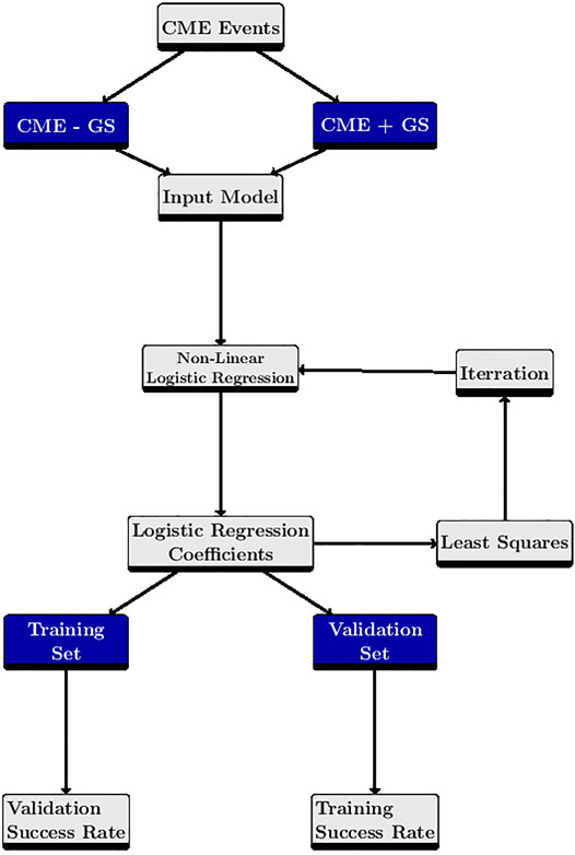
FIGURE 1. A.I. flow.

2.3 Selection of Independent Variables

We studied all the properties listed in the LASCO catalogue linear speed, second order speed at final height, second order speed at 20 solar radii, the central and measured position angle, the angular width, the acceleration, the mass and energy of the CME.

We eliminated variables that correlated amongst them. The full correlation tables of all CME parameters can be found in Besliu-Ionescu et al. (2019). We selected parameters with small correlation coefficients such that the non-linear logistic regression is correctly applied. We decided to exclude the linear speed as there is supporting evidence (Verma et al., 2013) that the correlation between the linear speed of the CME and the Dst index is weak. There were two classes of variables that were correlated: the three types of CME velocities ($V_{lin}$, $V_{20R}$ and $V_{2f}$) and the two angles–measured and central position angles (MPA and CPA). We chose one per each class. The speed at 20 solar radii better represents the state of the CME after escaping the solar corona. Then, we eliminated the mass and energy of the CME because of the large uncertainties due to poor measurements.

Hence, in this study the new set of independent variables consisted of: the speed of the CME at 20 solar radii, its angular width, measured position angle, acceleration and the location of the source region. The location bin variable was set to be 0 if the source was on the backside of the Sun, and 1 if the source was on the frontside, disregarding its exact latitude and longitude. Thus our dataset of 2,796 CMES consists of 1,647 frontside CMEs and 1,149 backside ones.

The measurements that were not binary variables defined (speed at 20 solar radii, measured position angle and angular width) were normalized to unity in order to minimize the possible numerical errors or discrepancies due to the variable ranges.

We also used a set of standardized data computed by removing the mean and dividing by the standard deviation (e.g., Gelman, 2008) (denoted by *ST in Table 1).

TABLE 1

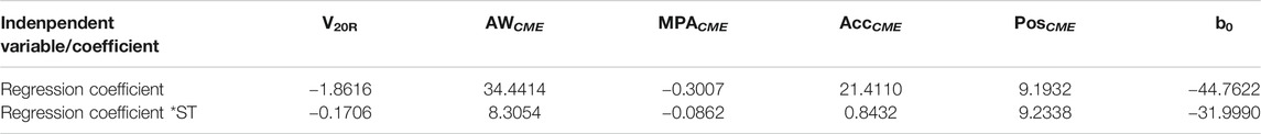
TABLE 1. The resulting logistic regression coefficients following the non-linear logistic regression model for normalized values (first row) and for standardized values (second row).

3 Results

The output after running the non-linear logistic regression model are the six coefficients, b₀ … b₅ (see Eqs 2–4) which are also displayed in Table1.

$\begin{array}{c}{Z}_i=-44.7622-1.8616\times V_{20R}+34.4414\times A{W}_{CME}\\ -0.3007\times MP{A}_{CME}+9.1932\times PO{S}_{CME}\end{array}(3)$

$\begin{array}{c}{Z}_i(\ast ST)=31.9990-0.1706\times V_{20R}+8.3054\times A{W}_{CME}\\ -0.0862\times MP{A}_{CME}+9.2338\times PO{S}_{CME}\end{array}(4)$

Choosing standardized input data puts all predictors on a common scale (Gelman, 2008) allowing us to compare the resulting logistic regression coefficients. The classification of coefficients as response given by predictors between the two methods of preparing the data is very similar. The difference between them consists in the order of the first three predictors–the source position, the acceleration and the angular width.

Choosing the normalization method of data preparation suggest that the CME angular width is the most important predictor, while choosing the standardization method, the most important one is the CME source position.

The other predictors have the same importance in both methods. The residual sum of squares for both methods has the same value.

The presented set of independent variables was selected because it had the smallest residual sum of squares value. The residual sum of squares was calculated by IDL and stored into the SSE variable.

Other sets that we have tried were: [$Vli{n}_{CME}$, $CP{A}_{CME}$, $A{W}_{CME}$, $Ac{c}_{CME}$, $RSSn$], [$V2f_{CME}$, $CP{A}_{CME}$, $A{W}_{CME}$, $A{W}_{CME}$, $RSSn$], [$V20R_{CME}$, $CP{A}_{CME}$, $A{W}_{CME}$, $Ac{c}_{CME}$, $RSSn$], [$V2f_{CME}$, $MP{A}_{CME}$, $A{W}_{CME}$, $A{W}_{CME}$, $RSSn$] [$V2f_{CME}$, $MP{A}_{CME}$, $A{W}_{CME}$, $A{W}_{CME}$, $RSSn$], [$V2f_{CME}$, $MP{A}_{CME}$, $A{W}_{CME}$, $A{W}_{CME}$, $RSSn$]. In this notations, $V_{lin}$ is the linear speed of the CME, $V2f_{CME}$ second order speed at final height, $RSSn$ the smoothed sunspot number.

3.1 Training Set

As already mentioned, we divided the events into the two categories needed for running the model, training and validation, three fourths for the training one, and the remaining one fourth for the validation one.

Thus, the training set contained 2,097 events, with 33 positive events included. By positive event we define a CME that reached the Earth and that was associated with a geomagnetic storm (i.e., a minimum Dst value $\mathrm{⩽}$ −30 nT). The vast majority of the events (2,763) were negative events, meaning that CMEs never reached the Earth, or they were not associated with a geomagnetic storm.

Using the coefficients displayed in Table 1 we have computed the probability that a geomagnetic storm is produced (Formula 1) for each considered event using the regression model.

$\text{Π}$ is the probability of the occurrence of a geomagnetic storm (Dst $\mathrm{⩽}$ −30 nT). If $\text{Π}$ is bigger than 50% then we considered that a geomagnetic storm was forecasted by the model and if $\text{Π}$ is smaller than 50% then there was no geomagnetic storm. A correct forecast will mean a probability bigger than 50% for a positive event and a probability less than 50% for a negative event. Hence, the success rate was computed as the number of correct forecasts divided by the total number of events. The general success rate (considering both positive and negative events) was 0.986, and 0.987, respectively for the normalized and standardized set. During training, the model did not successfully predict any of the 27 positive events.

3.2 Validation Set

The validation set contained 699 events with six positive events included. For this set the success rate was 0.989 and 0.989, respectively for the normalized and standardized set. The validation set din not correctly forecasted any of the six CMEs that were associated with geomagnetic storms.

4 Discussion

4.1 CME Activity During SC24

In order to study the geoeffectiveness of our 2,796 CMEs during SC24, we have attempted a statistical analysis of the CME evolution with the solar cycle. Figure 2 shows in the left panel the annual number of detected CMEs in blue bars and the yearly smoothed sunspot number in a black line.

FIGURE 2

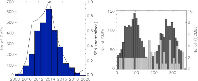
FIGURE 2. (A): Total number of CMEs per year (blue histograms) and yearly smoothed sunspot number (black line). (B): The measured position angle for all CMEs studied here during 2008–2020 (black histograms) and for CMEs that have reached the interplanetary space (gray histograms).

Every aspect of the solar activity varies during the 11-years solar cycle. Taking the sunspot number as the most significant indicator of the cycle’s activity, this would mean that coronal mass ejections will also vary with the sunspot number, either in correlation or anticorrelation. Figure 2 shows a good correlation between the number of detected CMEs and the sunspot number.

Solar cycle 24 began on January 1, 2007 with its ascending phase lasting fifteen months until April 1, 2010. Solar cycle’s maximum phase started on July 1, 2011 and ended on March 31, 2015. It had two maxima on October 2013 and February 2014. The descending phase ended on July 31, 2017. The maximum number of detected CMEs coincides with the year of the maximum monthly smoothed sunspot number. In another study, no significant correlation between the phases of solar cycle and yearly occurrence of intense and great storms has been found (Rathore and Parashar, 2011).

Generally, the yearly number of detected CMEs follows the yearly smoothed sunspot number as seen in Figure 2. It is clearly observable that there are less CMEs detected during the descending phase of SC24 by comparison with its ascending phase.

We have observed that 68% of the CMEs were detected during the maximum phase of the solar cycle and that the descending phase had the least events–only 10%. Similarly, high speed CMEs (the speed at 20 solar radii exceeding 1,000 km/s) were significantly more during the maximum phase of the cycle (129), while the descending phase had the smallest number (20).

Considering CMEs from the point of view of the MPA, there are more CMEs measured in the northern hemisphere–with $\sim$8% more than the sourthern one. The explicit division as a function of the MPA is 28% in the NE quadrant, 26% NW quadrant, 24 and 22%, respectively for the southern ones (SE/SW). This difference is considered to be too small to be motivated by a certain preference.

The right panel of Figure 2 shows a histogram that represents in dark gray the total number of CMEs and in light gray the CMEs which arrived at the Earth (ICMEs) as a function of their measured position angle. This histogram is constructed in bins of 10 degrees for all CMEs studied here and shows a preference for 80–120$°$ and 260–300$°$ latitudinal bands.

The slight preference for the northern hemisphere is not reproduced for the CMEs that were detected near Earth. There were 15 CMEs coming from regions near the poles ($\pm$30$°$) that reached the Earth, and only nine have produced geomagnetic storms.

Nine out of these 15 ICMEs were detected during the maximum phase of SC24, which is contrary to the fact that most of the ICMEs were detected during the descending phase (29 ICMEs out of the 49 included in our set). 21 were followed by geomagnetic storms. Halo CMEs are most geoeffective between the maximum and descending phases of SC23 (Shrivastava, 2011). Zhang et al. (2008) found similar results for CIRs during the descending phase of SC23.

Gopalswamy et al. (2020) analyzed 44 and 38 limb halo CMEs in cycles 23 and 24, respectively, in order to quantify the effect of the heliospheric influence on CME properties. Their study reveals the effect of the reduced total pressure in the heliosphere that allows cycle 24 CMEs to expand more and become halos sooner than those from cycle 23. They also found similar results regarding the CME activity during the solar cycle, more specifically, that the maximum number of detected CMEs coincides with the maximum value of the relative sunspot number, which can easily be confirmed from Figure 2.

A better understanding of the linkage between CMEs and solar activity cycle should improve our understanding about their geoeffectiveness. Some studies (e.g., Wang et al., 2002; Echer et al., 2008; Rathore and Parashar, 2011; Verma et al., 2013) show that there are more geomagnetic storms related to eruptive phenomena during the descending phase of a solar cycle.

A classification of CMEs by their linear speed into three categories (v $<$ 250, 250 $\mathrm{⩽}$ v $<$ 1,000, v $\mathrm{⩽}$ 1,000 km/s, respectively) led Miteva et al. (2017) to see the same coincidence between the number of CMEs and the sunspot number. They also confirm that SC24 was low in 25–50 MeV proton events, X-to-C class solar flares and faster than 1,000 km/s CMEs, all these phenomena being reduced by 30–45% with respect to SC23.

Our study has 1,352 CMEs coming from the western hemisphere and 1,444 from the eastern one. Out of these, there were 23 ICMEs and 26, respectively. Cycle 24 lacks in events driving extreme geomagnetic storms compared to past solar cycles. Out of the 49 ICMEs included in our study, 33 have been followed by geomagnetic storms.

For solar cycle 24 Hess and Zhang (2017) have identified 70 Earth-affecting interplanetary coronal mass ejections (ICMEs). They found that Earth-affecting CMEs in the first half of Cycle 24 are more likely to come from the northern hemisphere, but after April 2012, it reverses. They also found that in past solar cycles, CMEs from the western hemisphere were more likely to reach Earth.

Only around 50% of the ICMEs were generating GSs during the years 1996–2017. Out of these, around 23% generated intense GSs (with Dst $\mathrm{⩽}$ −100 nT) and the probability for severe storms (Dst $\mathrm{⩽}$ −200 nT) was 4% (Alexakis and Mavromichalaki, 2019). Similar results were found also by Richardson and Cane (2011) for the time period 1995–2009. For our selected events the percentage of ICMEs followed by geomagnetic storms, including minor ones, is $\sim$67%.

In our dataset containing 49 ICMEs there are nine intense geomagnetic storms associated with them, and only one severe storm (Dst_min = −223 nT). This means that $\sim$ 59% of ICMEs were followed by geomagnetic storms.

Using a Spearman rank correlation coefficient between Dst index and CME speed for 33 halo CMEs from the beginning of the past solar cycle (2009–2013). Bisht et al. (2017) showed that high speed CMEs and big flares are not the effective and significant parameters for the geoeffectiveness of these selected halo events. This supported our decision for eliminating the parameter related to the flare-CME association.

In our study, out of the 2,796 CMEs, there were 276 halo ones, out of which 24 were associated with geomagnetic storms, having velocities ranging from 143 to 3,163 km/s. This resulted in a 0.08 Spearman coefficient between the linear speed and the Dst index.

In a propagation through the interplanetary space analysis of 53 fast Earth-directed halo CMEs observed by the LASCO instrument during the period January 2009–September 2015 Scolini et al. (2018) found that 82% of the CMEs arrived at Earth in the next 4 days. The events were propagated to 1AU by means of the WSA-ENLIL +Cone model and almost all of them triggered geomagnetic storms. The average time delay in the case of our geoeffective CMEs was $\sim$3 days.

No other statistics of the measured CME properties have shown a noticeable dependence of the solar cycle evolution.

4.2 Concluding Remarks

We have applied a non-linear logistic regression model to a selected set of CMEs detected by LASCO in order to evaluate their geoeffectiveness such as defined by their association to a geomagnetic storm. The selected CMEs excluded “poor” and “very poor” events and CMEs with angular width less than 60$°$, thus obtaining a database of 2,796 events. These CMEs were divided into training (three quarters) and validation (one quarter) sets. Using a set of five independent variables (V_20R, AW_CME, MPA_CME, Acc_CME, Pos_CME), the correlation to ICMEs and geomagnetic storms according to the ICME catalogue (Richardson and Cane, 2011), we have computed the probability that a CME will be associated with a geomagnetic storm. We normalized and standardized the input data such that we minimize the numerical errors. We have obtained greater than 0.98 success rates for all categories. However, there were no positive events correctly forecasted.

Besides CME-CME interaction there is now an increasing concern that stealth CMEs are also important from the space weather perspective (e.g., Nitta and Mulligan, 2017; Mishra and Srivastava, 2019). The stealth CMEs lack any low coronal signatures (see e.g., Robbrecht et al., 2009; D’Huys et al., 2014) which is why they are more difficult to forecast if they erupt from the visible part of the Sun and if they arrive at Earth. Such CMEs have an important physical concern for other planetary magnetospheres as well (see e.g., Thampi et al., 2021). Our model forecasted that stealth CMEs will not have any impact on the Earth, as their location was originating from the backside.

As the stealth CMEs are lacking low-coronal signatures, their source regions could not be identified. In consequence, these CMEs were considered as originating from the backside of the Sun (location variable was set to 0). This implies that our model will not forecast that stealth CMEs will have any impact on the Earth.

During their journey from the Sun to the Earth, CMEs can accelerate/decelerate, deflect, rotate and deform (see e.g., Manchester et al., 2014; Manchester et al., 2017). Syed Ibrahim et al. (2019) found that the ICME transit-time decreases with the increase in the CME initial speed, although a broad range of transit times were observed for a given CME speed. For slow CMEs ($<$400 km/s), the energy is transferred from the solar wind to the CMEs, while faster events ($\mathrm{⩾}$400 km/s) tend to lose their energy to the ambient medium (e.g., Soni et al., 2019).

The paragraphs above reveal the limitation of our model by using only the CME parameters as input for the model. A possible improvement might be the addition of some weighting coefficients to increase the significance of the positive events in the training process. For a more robust analysis one also needs to take into consideration the interaction between the CMEs and the ambient solar wind during their journey to the Earth. Throughout their propagation, the CME parameters like speed, shape, etc. change considerably and this has a big impact on their geoeffective response.

However, we consider this model to be a sustainable one for the purpose of predicting the association of a geomagnetic storm to a CME which arrived at Earth, based solely on the measurements of the CME’s properties.

Another improvement of this model could be the addition of the tilt angle of the CME to the dataset, in order to better estimate the direction of the CME propagation, even though it will not take into consideration the interplanetary interactions.

Data Availability Statement

The raw data supporting the conclusions of this article will be made available by the authors, without undue reservation.

Author Contributions

DB-I contributed to construction of database, running the model, main writer of the text. MM contributed to construction of database, writing and reviewing text and software.

Funding

Part of DB-I’s work was supported by a grant of the Romanian Ministery of Research and Innovation, CCCDI - UEFISCDI, project number PN-III-P1-1.2-PCCDI-2017-0226/16PCCDI/2018, within PNCDI III.

Conflict of Interest

The authors declare that the research was conducted in the absence of any commercial or financial relationships that could be construed as a potential conflict of interest.

Acknowledgments

The CME LASCO catalog is generated and maintained at the CDAW Data Center by NASA and The Catholic University of America in cooperation with the Naval Research Laboratory. SOHO is a project of international cooperation between ESA and NASA.

References

Alexakis, P., and Mavromichalaki, H. (2019). Statistical Analysis of Interplanetary Coronal Mass Ejections and Their Geoeffectiveness During the Solar Cycles 23 and 24. Astrophys. Space Sci. 364, 187. doi:10.1007/s10509-019-3677-y

CrossRef Full Text | Google Scholar

Besliu-Ionescu, D., Talpeanu, D.-C., Mierla, M., and Muntean, G. M. (2019). On the Prediction of Geoeffectiveness of CMEs During the Ascending Phase of SC24 Using a Logistic Regression Method. J. Atmos. Solar-Terrestrial Phys. 193, 105036. doi:10.1016/j.jastp.2019.04.017

CrossRef Full Text | Google Scholar

Bhatt, B., and Chandra, H. (2020). Relationship Between Rising Phase of Solar Cycle 23rd and 24th With Respect to Geoeffectiveness. Adv. Sci. Engng Med. 12, 70–74. doi:10.1166/asem.2020.2518

CrossRef Full Text | Google Scholar

Bisht, H., Pande, B., Chandra, R., and Pande, S. (2017). Geoeffectiveness of Solar Eruptions During the Rising Phase of Solar Cycle 24. New Astron. 51, 74–85. doi:10.1016/j.newast.2016.08.014

CrossRef Full Text | Google Scholar

Bruevich, E. A., and Yakunina, G. V. (2020). 24th Cycle of Solar Activity: Geoefficiency of Flares. Geomagn. Aeron. 60, 876–880. doi:10.1134/S0016793220070087

CrossRef Full Text | Google Scholar

Cane, H. V., and Richardson, I. G. (2003). Interplanetary Coronal Mass Ejections in the Near-Earth Solar Wind During 1996–2002. J. Geophys. Res. 108, 1156. doi:10.1029/2002JA009817

CrossRef Full Text | Google Scholar

Chi, Y., Shen, C., Wang, Y., Xu, M., Ye, P., and Wang, S. (2016). Statistical Study of the Interplanetary Coronal Mass Ejections from 1995 to 2015. Sol. Phys. 291, 2419–2439. doi:10.1007/s11207-016-0971-5

CrossRef Full Text | Google Scholar

D’Huys, E., Seaton, D. B., Poedts, S., and Berghmans, D. (2014). Observational Characteristics of Coronal Mass Ejections Without Low-Coronal Signatures. Astrophysical J. 795, 49. doi:10.1088/0004-637X/795/1/49

CrossRef Full Text | Google Scholar

Echer, E., Gonzalez, W. D., Tsurutani, B. T., and Gonzalez, A. L. C. (2008). Interplanetary Conditions Causing Intense Geomagnetic Storms (Dst ≤ −100 nT) During Solar Cycle 23 (1996–2006). J. Geophys. Res. 113, A05221. doi:10.1029/2007JA012744

CrossRef Full Text | Google Scholar

Gelman, A. (2008). Scaling Regression Inputs by Dividing by Two Standard Deviations. Statist. Med. 27, 2865–2873. doi:10.1002/sim.3107

CrossRef Full Text | Google Scholar

Gonzalez, W. D., Joselyn, J. A., Kamide, Y., Kroehl, H. W., Rostoker, G., Tsurutani, B. T., et al. (1994). What is a Geomagnetic Storm? J. Geophys. Res. 99, 5771–5792. doi:10.1029/93JA02867

CrossRef Full Text | Google Scholar

Gopalswamy, N., Akiyama, S., Yashiro, S., and Makela, P. (2010). Coronal Mass Ejections from Sunspot and Non-Sunspot Regions. Astrophy. Space Sci. Proc. 19, 289–307. doi:10.1007/978-3-642-02859-5_24

CrossRef Full Text | Google Scholar

Gopalswamy, N., Yashiro, S., and Akiyama, S. (2007). Geoeffectiveness of Halo Coronal Mass Ejections. J. Geophys. Res. 112, A06112. doi:10.1029/2006JA012149

CrossRef Full Text | Google Scholar

Gopalswamy, N., Mäkelä, P., Xie, H., and Yashiro, S. (2013). Testing the Empirical Shock Arrival Model Using Quadrature Observations. Space Weather 11, 661–669. doi:10.1002/2013SW000945

CrossRef Full Text | Google Scholar

Gopalswamy, N., Akiyama, S., and Yashiro, S. (2020). The State of the Heliosphere Revealed by Limb-Halo Coronal Mass Ejections in Solar Cycles 23 and 24. Astrophys. J., Lett. 897, L1. doi:10.3847/2041-8213/ab9b7b

CrossRef Full Text | Google Scholar

Hess, P., and Zhang, J. (2017). A Study of the Earth-Affecting CMEs of Solar Cycle 24. Sol. Phys. 292, 80. doi:10.1007/s11207-017-1099-y

CrossRef Full Text | Google Scholar

Joshi, N. C., Uddin, W., Srivastava, A. K., Chandra, R., Gopalswamy, N., Manoharan, P. K., et al. (2013). A Multiwavelength Study of Eruptive Events on January 23, 2012 Associated With a Major Solar Energetic Particle Event. Adv. Space Res. 52, 1–14. doi:10.1016/j.asr.2013.03.009

CrossRef Full Text | Google Scholar

Kilpua, E. K. J., Mierla, M., Zhukov, A. N., Rodriguez, L., Vourlidas, A., and Wood, B. (2014). Solar Sources of Interplanetary Coronal Mass Ejections During the Solar Cycle 23/24 Minimum. Sol. Phys. 289, 3773–3797. doi:10.1007/s11207-014-0552-4

CrossRef Full Text | Google Scholar

Kraaikamp, E., and Verbeeck, C. (2015). Solar Demon - an Approach to Detecting Flares, Dimmings, and euv Waves on sdo/aia Images. J. Space Weather Space Clim. 5, A18. doi:10.1051/swsc/2015019

CrossRef Full Text | Google Scholar

Lamy, P. L., Floyd, O., Boclet, B., Wojak, J., Gilardy, H., and Barlyaeva, T. (2019). Coronal Mass Ejections over Solar Cycles 23 and 24. Space Sci. Rev. 215, 39. doi:10.1007/s11214-019-0605-y

CrossRef Full Text | Google Scholar

Manchester, W., Kilpua, E. K. J., Liu, Y. D., Lugaz, N., Riley, P., Török, T., et al. (2017). The Physical Processes of CME/ICME Evolution. Space Sci. Rev. 212, 1159–1219. doi:10.1007/s11214-017-0394-0

CrossRef Full Text | Google Scholar

Manchester, W. B., van der Holst, B., and Lavraud, B. (2014). Flux Rope Evolution in Interplanetary Coronal Mass Ejections: the 13 May 2005 Event. Plasma Phys. Control Fusion 56, 064006. doi:10.1088/0741-3335/56/6/064006

CrossRef Full Text | Google Scholar

Maris, G., Popescu, M.-D., and Mierla, M. (2002). “Geomagnetic Consequences of the Solar Flares During the Last Hale Solar Cycle (II),”. in Solspa 2001, Proceedings of the Second Solar Cycle and Space Weather Euroconference, Vico Equense, Italy, September 24–29, 2001. Editor H. Sawaya-Lacoste (Noordwijk, Netherlands: ESA Special Publication), 477, 451–454.

Google Scholar

Mishra, S. K., and Srivastava, A. K. (2019). Linkage of Geoeffective Stealth CMEs Associated With the Eruption of Coronal Plasma Channel and Jet-Like Structure. Sol. Phys. 294, 169. doi:10.1007/s11207-019-1560-1

CrossRef Full Text | Google Scholar

Miteva, R., Samwel, S. W., Costa-Duarte, M. V., and Malandraki, O. E. (2017). Solar Cycle Dependence of Wind/EPACT Protons, Solar Flares and Coronal Mass Ejections. Sun Geosphere 12, 11–19.

Google Scholar

Möstl, C., Weiss, A. J., Bailey, R. L., Reiss, M. A., Amerstorfer, T., Hinterreiter, J., et al. (2020). Prediction of the In Situ Coronal Mass Ejection Rate for Solar Cycle 25: Implications for Parker Solar Probe In Situ Observations. Astrophys. J. 903, 92. doi:10.3847/1538-4357/abb9a1

CrossRef Full Text | Google Scholar

Nakagawa, T., Gopalswamy, N., and Yashiro, S. (2006). Solar Wind Speed Within 20RSof the Sun Estimated from Limb Coronal Mass Ejections. J. Geophys. Res. 111, A01108. doi:10.1029/2005JA011249

CrossRef Full Text | Google Scholar

Nitta, N. V., and Mulligan, T. (2017). Earth-Affecting Coronal Mass Ejections Without Obvious Low Coronal Signatures. Sol. Phys. 292, 125. doi:10.1007/s11207-017-1147-7

CrossRef Full Text | Google Scholar

Paraschiv, A. R., Lacatus, D. A., Badescu, T., Lupu, M. G., Simon, S., Sandu, S. G., et al. (2010). Study of Coronal Jets During Solar Minimum Based on STEREO/SECCHI Observations. Sol. Phys. 264, 365–375. doi:10.1007/s11207-010-9584-6

CrossRef Full Text | Google Scholar

Raouafi, N. E., Patsourakos, S., Pariat, E., Young, P. R., Sterling, A. C., Savcheva, A., et al. (2016). Solar Coronal Jets: Observations, Theory, and Modeling. Space Sci. Rev. 201, 1–53. doi:10.1007/s11214-016-0260-5

PubMed Abstract | CrossRef Full Text | Google Scholar

Rathore, B. S., Kaushik, S. C., Parashar, K., Bhadoria, R. S., and Kapil, P. (2011). Statistical Study of Geomagnetic Storms and Their Classification During Solar Cycle-23. Int. J. Phys. Appl. 3, 91–96.

Google Scholar

Richardson, I. G., and Cane, H. V. (2010). Near-Earth Interplanetary Coronal Mass Ejections During Solar Cycle 23 (1996–2009): Catalog and Summary of Properties. Sol. Phys. 264, 189–237. doi:10.1007/s11207-010-9568-6

CrossRef Full Text | Google Scholar

Richardson, I. G., and Cane, H. V. (2011). Geoeffectiveness (Dst and Kp) of Interplanetary Coronal Mass Ejections During 1995–2009 and Implications for Storm Forecasting. Space Weather 9, S07005. doi:10.1029/2011SW000670

CrossRef Full Text | Google Scholar

Robbrecht, E., Patsourakos, S., and Vourlidas, A. (2009). No Trace Left Behind: Stereo Observation of a Coronal Mass Ejection Without Low Coronal Signatures. Astrophys. J. 701, 283–291. doi:10.1088/0004-637X/701/1/283

CrossRef Full Text | Google Scholar

Schwenn, R. (2006). Space Weather: The Solar Perspective. Living Rev. Solar Phys. 3, 2. doi:10.12942/lrsp-2006-2

CrossRef Full Text | Google Scholar

Scolini, C., Chané, E., Temmer, M., Kilpua, E. K. J., Dissauer, K., Veronig, A. M., et al. (2020). CME-CME Interactions as Sources of CME Geoeffectiveness: The Formation of the Complex Ejecta and Intense Geomagnetic Storm in 2017 Early September. Astrophys. J. Supple. Ser. 247, 21. doi:10.3847/1538-4365/ab6216

CrossRef Full Text | Google Scholar

Scolini, C., Messerotti, M., Poedts, S., and Rodriguez, L. (2018). Halo Coronal Mass Ejections during Solar Cycle 24: Reconstruction of the Global Scenario and Geoeffectiveness. J. Space Weather Space Clim. 8, A09. doi:10.1051/swsc/2017046

CrossRef Full Text | Google Scholar

Shen, C., Xu, M., Wang, Y., Chi, Y., and Luo, B. (2018). Why the Shock-ICME Complex Structure is Important: Learning From the Early 2017 September CMEs. Astrophys. J. 861, 28. doi:10.3847/1538-4357/aac204

CrossRef Full Text | Google Scholar

Shrivastava, P. K., and Mishra, B. K. (2011). Geoeffectiveness of Halo CMEs During Different Phases of Solar Activity Cycle 23. Int. Cosmic Ray Conf. 11, 280. doi:10.7529/ICRC2011/V11/0070

CrossRef Full Text | Google Scholar

Soni, S. L., Singh, P. R., Nigam, B., Gupta, R. S., and Shrivastava, P. K. (2019). The Analysis of Interplanetary Shocks Associated with Six Major Geo-Effective Coronal Mass Ejections during Solar Cycle 24. Int. J. Astron. Astrophys. 09, 191–199. doi:10.4236/ijaa.2019.93014

CrossRef Full Text | Google Scholar

Srivastava, N. (2005). A Logistic Regression Model for Predicting the Occurrence of Intense Geomagnetic Storms. Ann. Geophys. 23, 2969–2974. doi:10.5194/angeo-23-2969-2005

CrossRef Full Text | Google Scholar

Srivastava, N., and Venkatakrishnan, P. (2004). Solar and Interplanetary Sources of Major Geomagnetic Storms during 1996–2002. J. Geophys. Res. 109, A10103. doi:10.1029/2003JA010175

CrossRef Full Text | Google Scholar

Syed Ibrahim, M., Joshi, B., Cho, K.-S., Kim, R.-S., and Moon, Y.-J. (2019). Interplanetary Coronal Mass Ejections During Solar Cycles 23 and 24: Sun-Earth Propagation Characteristics and Consequences at the Near-Earth Region. Sol. Phys. 294, 54. doi:10.1007/s11207-019-1443-5

CrossRef Full Text | Google Scholar

Thampi, S. V., Krishnaprasad, C., Nampoothiri, G. G., and Pant, T. K. (2021). The Impact of a Stealth CME on the Martian Topside Ionosphere. Monthly Notices R. Astronom. Soc. 503, 625–632. doi:10.1093/mnras/stab494

CrossRef Full Text | Google Scholar

Verma, R., Kumar, S., and Dubey, S. (2013). Coronal Mass Ejection, Magnetic Cloud and Their Geoeffectiveness During 1996–2009. Int. J. Sci. Res. 5, 1832–1836.

Google Scholar

Wang, Y. M., Ye, P. Z., Wang, S., Zhou, G. P., and Wang, J. X. (2002). A Statistical Study on the Geoeffectiveness of Earth-Directed Coronal Mass Ejections from March 1997 to December 2000. J. Geophys. Res. 107, 1340. doi:10.1029/2002JA009244

CrossRef Full Text | Google Scholar

Webb, D. F., and Howard, T. A. (2012). Coronal Mass Ejections: Observations. Living Rev. Solar Phys. 9, 3. doi:10.12942/lrsp-2012-3

CrossRef Full Text | Google Scholar

Xu, M., Shen, C., Wang, Y., Luo, B., and Chi, Y. (2019). Importance of Shock Compression in Enhancing ICME's Geoeffectiveness. Astrophys. J. Lett. 884, L30. doi:10.3847/2041-8213/ab4717

CrossRef Full Text | Google Scholar

Yashiro, S., Gopalswamy, N., Akiyama, S., and Mӓkelӓ, P. A. (2020). A Catalog of Prominence Eruptions Detected Automatically in the SDO/AIA 304 Å Images. J. Atmos. Solar-Terrestrial Phys. 205, 105324. doi:10.1016/j.jastp.2020.105324

CrossRef Full Text | Google Scholar

Yashiro, S., Gopalswamy, N., Michalek, G., Cyr, St. O. C., Plunkett, S. P., Rich, N. B., et al. (2004). A Catalog of White Light Coronal Mass Ejections Observed by the SOHO Spacecraft. J. Geophys. Res. 109, A07105. doi:10.1029/2003JA010282

CrossRef Full Text | Google Scholar

Zhang, J., Richardson, I. G., Webb, D. F., Gopalswamy, N., Huttunen, E., Kasper, J. C., et al. (2007). Solar and Interplanetary Sources of Major Geomagnetic Storms (Dst≤ −100 nT) During 1996–2005. J. Geophys. Res. 112, A10102. doi:10.1029/2007JA012321

CrossRef Full Text | Google Scholar

Zhang, Y., Sun, W., Feng, X. S., Deehr, C. S., Fry, C. D., and Dryer, M. (2008). Statistical Analysis of Corotating Interaction Regions and Their Geoeffectiveness during Solar Cycle 23. J. Geophys. Res. 113, A08106. doi:10.1029/2008JA013095

CrossRef Full Text | Google Scholar