 Sabrina Guastavino
 Francesco Marchetti
 Federico Benvenuto1
 Cristina Campi
 Michele Piana
- 1MIDA, Dipartimento di Matematica, Università di Genova, Genova, Italy
- 2Dipartimento di Matematica “Tullio Levi Civita”, Università di Padova, Padova, Italy
- 3INAF–Osservatorio Astrofisico di Torino, Torino, Italy
Operational flare forecasting aims at providing predictions that can be used to make decisions, typically on a daily scale, about the space weather impacts of flare occurrence. This study shows that video-based deep learning can be used for operational purposes when the training and validation sets used for network optimization are generated while accounting for the periodicity of the solar cycle. Specifically, this article describes an algorithm that can be applied to build up sets of active regions that are balanced according to the flare class rates associated to a specific cycle phase. These sets are used to train and validate a long-term recurrent convolutional network made of a combination of a convolutional neural network and a long short-term memory network. The reliability of this approach is assessed in the case of two prediction windows containing the solar storms of March 2015, June 2015, and September 2017.
1 Introduction
Solar flare prediction is an important task in the context of space weather research as it addresses open problems in both solar physics and operational forecasting (Schwenn, 2006; McAteer et al., 2010). Although it is well established that solar flares are a consequence of reconnection and reconfiguration of magnetic field lines high in the solar corona (Shibata, 1996; Sui et al., 2004; Su et al., 2013), there is still no agreement about the physical model that better explains the sudden magnetic energy release and the resulting acceleration mechanisms (Shibata, 1996; Sui et al., 2004; Aschwanden, 2008; Su et al., 2013). Furthermore, solar flares are the main trigger of other space weather phenomena, and it is a challenging forecasting issue to predict the chain of events leading from solar flares to possible significant impacts on both in-orbit and on-Earth assets (Crown, 2012; Murray et al., 2017).
Flare forecasting relies on both statistical (Song et al., 2009; Mason and Hoeksema, 2010; Bloomfield et al., 2012; Barnes et al., 2016) and deterministic (Strugarek and Charbonneau, 2014; Petrakou, 2018) methods. In the last decade, interest in machine and deep learning algorithms has grown, thanks to flexible algorithms that can take as input the point-in-time feature sets extracted from magnetograms, time series of features, point-in-time images of active regions, and videos whose frames are made of magnetograms (Bobra and Couvidat, 2015; Liu et al., 2017; Florios et al., 2018; Nishizuka et al., 2018; Campi et al., 2019; Liu et al., 2019; Li et al., 2020; Nishizuka et al., 2020, 2021; Georgoulis et al., 2021; Guastavino et al., 2022a; Pandey et al., 2022; Sun et al., 2022). However, Guastavino et al.(2022a) have pointed out that the prediction performances of these supervised approaches are characterized by a notable degree of heterogeneity, which is probably related to significant differences in the way data sets are generated for training and validation. This study introduced an original procedure for the generation of well-balanced training and validation sets and discussed its performances by means of a video-based deep learning approach that combined a convolutional neural network (CNN) with a long short-term memory (LSTM) network (Hochreiter and Schmidhuber, 1997).
The aim of our study is to show how that procedure can be used to build up an operational flare forecasting system that accounts for the periodicity of the solar activity. Specifically, applications are concerned with two temporal windows of the descent phase of Solar Cycle 24, comprising the “San Patrick’s Storm” that occurred in March 2015 (Astafyeva et al., 2015; Nayak et al., 2016; Wu et al., 2016), the storm in June 2015 (Joshi et al., 2018; Vemareddy, 2017), and the September 2017 storm (Guastavino et al., 2019; Qian et al., 2019; Benvenuto et al., 2020). Furthermore, we assessed the prediction accuracy by using both standard skill scores like the true skill statistic (TSS), the Heidke Skill Score (HSS), and the value-weighted skill scores introduced by Guastavino et al. (2022b), which better account for the intrinsic dynamic nature of forecasting problems (Guastavino et al., 2021; Hu et al., 2022). The results indicate that
• the construction of training and validation data sets whose composition reflects the flare occurrence rates of the test temporal window brings some benefits in terms of predictive accuracy, and
• the use of the value-weighted version of the TSS leads to predictions whose accuracy is comparable or higher than the ones provided by the standard TSS.
The plan of the article is as follows: Section 2 describes the data used for the analysis, the design of the neural network applied for the prediction, and the way operational flare forecasting is realized to account for solar cyclicity. Section 3 shows the results of the study. Our conclusions are offered in Section 4.
2 Material and methods
2.1 The data set
The archive of the Helioseismic and Magnetic Imager (HMI) (Scherrer et al., 2012) on board the Solar Dynamics Observatory (SDO) (Pesnell et al., 2011) contains two-dimensional magnetograms of continuous intensity, of the full three-component magnetic field vector and of the line-of-sight magnetic field. In our study, we considered the near-real-time Space Weather HMI Archive Patch (SHARP) data products that Bobra et al. (2014) associated to the line-of-sight components. Regarding an active region (AR), a sample associated to its history is a 24-hour-long video made of 40 SHARP images of an AR, with 36 min cadence and where each image has been resized to a 128 × 128 pixel dimension following a similar procedure used in Huang et al. (2018), Li et al. (2020), and Guastavino et al. (2022a) based on bilinear interpolation.
As in Guastavino et al. (2022a), we defined seven different types of videos. Denoting the X1+, M1+, and C1+, the classes of flares with class X1 or above, M1 or above, and C1 or above, respectively, we have that
• X-class samples are made of videos of ARs that originated from X1+ flares in the 24 h after the sample time.
• M-class samples are made of videos of ARs that, in the 24 h after the sample time, generated flares with M1+-class but below X-class.
• C-class samples are made of videos of ARs that, in the 24 h after the sample time, generate flares with C1+-class but below M-class.
• NO1 class samples are made of videos of ARs that never originated from a C1+ flare.
• NO2-class samples contain videos of ARs that originated a C1+ flare neither in the past nor in the 24 h after the sample time, but did originate in the future.
• NO3-class samples contain videos of ARs that did not originate a C1+ flare in the 24 h after the sample time, but originated a C1+ flare in the 48 h before the sample time [this definition accounts for the fact that relevant features like the flare index and flare past refer to the past 24 h window (Campi et al., 2019)].
• NO4-class samples contain videos of ARs that originated neither a C1+ flare in the 24 h after the sample nor a C1+ flare in the 48 h before the sample time, but originate a C1+ flare prior to 48 h before the sample time.
The first three types of samples describe the ability of ARs to generate flares of a given intensity in the following 24 h (which is the prediction time interval), whereas the last four types of videos are associated to ARs that did not generate significant flares in the same prediction interval. However, samples labeled with 0 may not represent a quiescent situation: for instance, NO3-class samples are associated to ARs that generated intense flares during the observation period. Therefore, it is considerably difficult to distinguish these types of NO samples from positive samples, which motivates the fact that they are often excluded from the analysis (Sun et al., 2022).
2.2 Neural network architecture
We used a deep neural network (DNN) which is appropriate for video classification. The DNN is called Long-term Recurrent Convolutional Network (LRCN) (Donahue et al., 2017); it is the combination of a convolutional neural network (CNN) and a recurrent neural network known as long short-term memory (LSTM) network. The architecture is the same as that used in Guastavino et al. (2022a) and is summarized in Table 1. Specifically, the CNN is characterized by the first four convolutional blocks with the number of nodes, kernel size, height and width strides, and activation function as the input parameters. Each convolutional layer is L2 regularized with the regularization level equal to 0.1. The output of the last max-pooling layer is flattened and given as the input to a fully connected layer of 64 units, where the dropout is applied with a fraction of 0.1 input units dropped. Therefore, the output of the CNNs is a time series of 64 features, which are then passed to the LSTM which consists of 50 units and where the dropout is applied with a fraction of 0.5 active units. Finally, the output of the LSTM layer is fed into the last fully connected layer, and the sigmoid activation function is applied to generate the probability distribution of the positive class in order to perform binary classification. The LRCN is trained over 100 epochs using the Adam Optimizer (Kingma and Ba, 2015), and the mini-batch size is equal to 128.
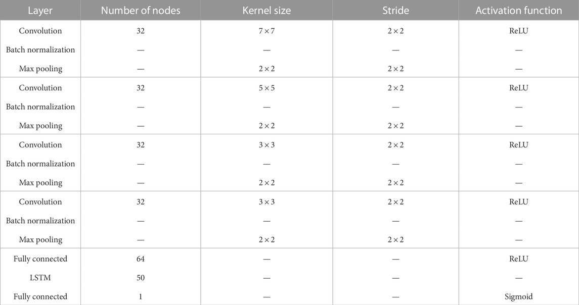
TABLE 1. Details of the LRCN architecture. The parameters of each layer, i.e., the number of filters, kernel size, height and width strides, and activation functions are shown.
2.3 Loss functions and skill scores
Loss functions and skill scores are intertwined concepts. On the one hand, in the training phase, loss functions should be chosen according to the learning task (Rosasco et al., 2004); on the other hand, in the validation/testing phase, skill scores should account for the properties of the training set and the overall nature of the learning problem. In the classification setting, skill scores are usually derived from the elements of the so-called confusion matrix (CM)
where the entries are the classical True Negative (TN), True Positive (TP), False Positive (FP), and False Negative (FN) elements. Score-Oriented Loss (SOL) functions were proposed in Marchetti et al. (2022) and applied in Guastavino et al. (2022a) for flare classification tasks. The concept at the basis of an SOL function is that it is defined starting from the definition of a skill score in such a way that the network optimization realized by means of that SOL function leads to the maximization of the corresponding skill score.
SOL functions are constructed by considering a probabilistic version
In the space weather community, true skill statistics (TSS) is a relevant score, which is defined as
and is appropriate in classifying problems characterized by class imbalance (TSS ranges in [ −1, 1] and is optimal when it is equal to 1). The SOL function associated to TSS is defined as
which is a differentiable function with respect to the weights of the network and is therefore eligible for use in the training phase.
In the applications considered in this study, the prediction accuracy has been assessed by means of both TSS and the Heidke Skill Score (HSS)
where P = TP + FN and N = TN + FP. The HSS measures the improvement of forecast over random forecast, ranges in (−∞, 1], and is optimal when it is equal to 1. Furthermore, we considered the value-weighted skill scores introduced in Guastavino et al. (2022b). These scores are based on a definition of the confusion matrix that assigns different weights to FPs (denoted by wFPs) and FNs (denoted by wFNs) in such a way that it accounts for the distribution of predictions along time with respect to the actual occurrences. By denoting the value-weighted confusion matrix as
predictions are assessed by computing the value-weighted TSS (wTSS) and value-weighted HSS (wHSS) defined as
The weights in the definitions of wFPs and wFNs allow mitigating errors such as false positives that precede the occurrence of an actual positive event and false negatives that are preceded by positive predictions.
They are defined as follows: let n be the number of samples, ordered on time, which are associated to a given AR. Moreover, let
where w ◦ t indicates the element-wise product. Then, wFP and wFN are defined as (cf. 2)
where
2.4 Operational flare forecasting
Machine learning theory (Vapnik, 1998) points out that training, validation, and test sets should be generated with samples drawn by means of the same probability distribution. However, in the case of flare forecasting, this requirement should account for the fact that solar periodicity introduces a bias in chronological splitting. Guastavino et al. (2022a) introduced an algorithm for the generation of training and validation sets based on proportionality (i.e., training set, validation set, and test set must have the same rate of samples for each sample type described in Section 2.1) and parsimony (i.e., each subset of samples must be provided by as few ARs as possible). This algorithm can be exploited in an operational setting if utilized, for example, as follows:
1) The current solar cycle is divided into three phases, in which the solar activity increases, reaches its maximum, and decreases, in that order.
2) Given a time point in the current solar cycle, the corresponding phase is identified.
3) For the same phase in the previous solar cycle, the algorithm computes the rates of the different sample types.
4) The training and validation sets are generated according to the sample rates from the whole data archive at disposal.
Then, the machine/deep learning method is trained by means of the generated training set, and the optimal epochs are chosen by means of the generated validation set. When the data set corresponding to the given time point is fed into the trained and validated neural network, flare prediction is performed for the following time point.
3 Results
3.1 Prediction for a test window
We considered two experiments, both concerning events occurred during Solar Cycle 24, involving
• the test window A: March–December 2015 (Nayak et al., 2016) and
• the test window B: January–September 2017 (Qian et al., 2019).
Both test windows are in the descent phase of Solar Cycle 24, therefore the approach discussed inSection 2.4 suggests computing the sample rates on a suitable window in the descent phase of the solar cycle. In order to comment on the effectiveness of the proposed setting, we compared such an approach with a different strategy where the sample rates were computed on a different phase of the solar cycle.
3.1.1 Same phase
The sample rates are computed on a tailored window in the descent phase of the solar cycle and before the test window was considered. Specifically,
• for the test window A, the rates of the video samples refer to the period from 30-04-2014 to 28-02-2015 and are pX ≈ 0.35%, pM ≈ 2.81%, pC ≈ 20.53%, pNO1 ≈ 33.25%, pNO2 ≈ 4.56%, pNO3 ≈ 17.89%, and pNO4 ≈ 20.61% (where pX denotes the rate of the X-class samples, pM denotes the rate of the M-class samples, and so on);
• for the test window B, the rates of the video samples refer to the period from 30-04-2014 to 28-12-2016 and are pX ≈ 0.16%, pM ≈ 3.18%, pC ≈ 16.82%, pNO1 ≈ 38.35%, pNO2 ≈ 5.49%, pNO3 ≈ 15.82%, and pNO4 ≈ 20.19%.
3.1.2 Different phases
The sample rates are computed on a window in the maximum phase of the solar cycle. Since the maximum phase is before both the two test windows A and B, we used the following unique period for the computation of sample rates: the rates of the video samples refer to the period from 30-04-2012 to 28-02-2015 and are pX ≈ 0.43%, pM ≈ 3.71%, pC ≈ 20.1%, pNO1 ≈ 30.55%, pNO2 ≈ 7.6%, pNO3 ≈ 16.77%, and pNO4 ≈ 20.86%.
The training and validation sets are generated as shown in Guastavino et al. (2022a) by randomly selecting ARs in a temporal training interval before the test window and by accounting for the rates computed in the previous step. In detail,
• for test window A, the ARs in the training and validation sets are taken from 14-09-2012 to 28-02-2015;
• for test window B, the ARs in the training and validation sets are taken from 14-09-2012 to 28-12-2016.
In the case of prediction of C1+ flares, we labeled the X-class, M-class, and C-class samples with 1 and the other ones with 0; in the case of prediction of M1+ flares, we labeled the X-class and M-class samples with 1 and the other ones with 0. The validation step was realized by selecting the epochs that provided the highest TSS and wTSS values. In the case of test window A, we found that the maximization of the two scores was obtained with the same epoch when the rates were computed on the same phase, leading to the same confusion matrix and the same skill score values on the test window (see column “Same phase rates” of Tables 2, 3). On the other hand, with regard to test window B, the epochs corresponding to the highest TSS and wTSS values were different, and the skill score values on the test window obtained by considering the wTSS were significantly higher (see column “Same phase rates” of Tables 4, 5). Furthermore, we noticed that for the test window A, the TSS and wTSS were higher when the sample rates were computed, referring to the same phase (see Tables 2, 3), whereas for the test window B, both skill scores and value-weighted skill scores were particularly high, independently of the chosen phase. This may be due to the fact that the year 2017 was characterized by a high percentage of X-class samples and NO1 samples, which are the easiest classes to be distinguished by a forecasting method. To facilitate the interpretation of the results at a glance, in each line of all tables, the best score is given in bold and the second-best score is underlined.
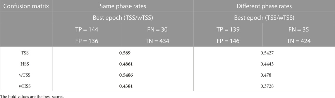
TABLE 2. Results on test window A for the prediction of C1+ flares. The epochs maximizing TSS and wTSS in the validation set are the same. The predictive model is defined with respect to this epoch.
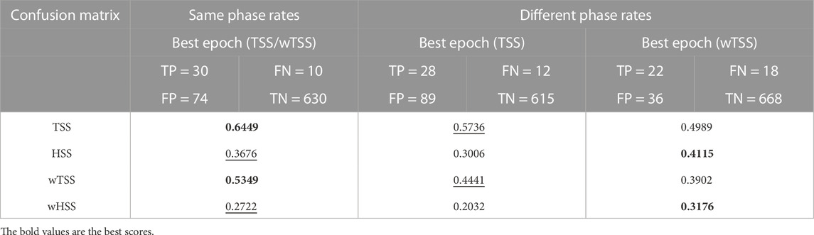
TABLE 3. Results on test window A for the prediction of M1+ flares. The epochs maximizing TSS and wTSS in the validation set are not the same in the different phase case.

TABLE 4. Results on test window B for the prediction of C1+ flares. In this case, the epochs maximizing TSS and wTSS in the validation set are different. The predictive models are defined with respect to these epochs, separately.
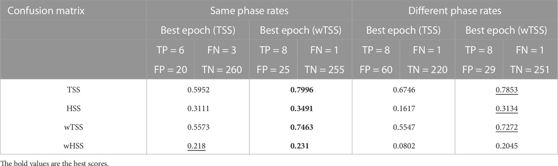
TABLE 5. Results on test window B for the prediction of M1+ flares. In this case, the epochs maximizing TSS and wTSS in the validation set are different. The predictive models are defined with respect to these epochs, separately.
3.2 A focus on storms
We consider three solar storms that occurred during test windows A and B. As far as the former is concerned, two storms associated to AR 12297 and AR 12371 occurred in March and June 2015, respectively (Astafyeva et al., 2015). Regarding test window B, in September 2017, a storm was linked to AR 12673 (Benvenuto et al., 2020). We finally focused on the prediction of these events by employing the same model constructed in the same phase case for the previous experiments. In all cases, the epochs corresponding to the highest TSS and wTSS lead to the same predictions.
Figure 1 shows the prediction enrolled over time associated to AR 12297. When the AR started generating C1+ flares, it is out from the field of view of the HMI, so the first prediction is made on 09-03-2015 00:00 for the next 24 h and the last prediction is made on 19-03-2015 for the next 24 h (after that date, the AR was out of the field of view of the HMI). The samples to predict associated to this AR are 1 X-, 8 M-, and 2 C-class samples. The algorithm correctly sent warnings of the C1+ flares from 09-03-2015 to 19-03-2015 and of the M1+ flares from 09-03-2015 to 17-03-2015. The M1+ flare warning given on 18-03-2015 is a false positive, but as the figure shows, a M1-class flare had just occurred (the peak time was on 17 March 2015, at 23:34). In Table 6, the confusion matrices are reported for C1+ and M1+ flare prediction.
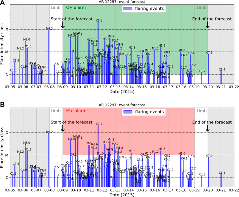
FIGURE 1. Predictions enrolled over time for the solar storm generated by AR 12297. The actual flaring events recorded by GOES, together with the corresponding GOES flare classes, are reported. The gray regions correspond to temporal windows out of the field of view of the HMI. (A) Warnings of C1+ flares are in green. (B) Warnings of M1+ flares are in red.

TABLE 6. Predictions of the solar storm associated to AR 12297. The first prediction was made on 3 March 2015, and the last one was on 19 March 2015.
Figure 2 shows the prediction enrolled over time associated to AR 12371. When the AR started generating C1+ flares, it is out from the field of view of the HMI, so the first prediction is made on 18-06-2015 00:00 for the next 24 h and the last prediction is made on 26-06-2015 for the next 24 h (after that date, the AR was out the field of view of the HMI). The samples to predict that are associated to this AR are 5 M-class and 9°C-class samples. The algorithm correctly predicted all the C-class samples, whereas we observed some false positives for M1+ flare predictions; we point out that such misclassifications belong to NO3-class samples. In Table 7, the confusion matrices are reported for the C1+ and M1+ flare prediction.
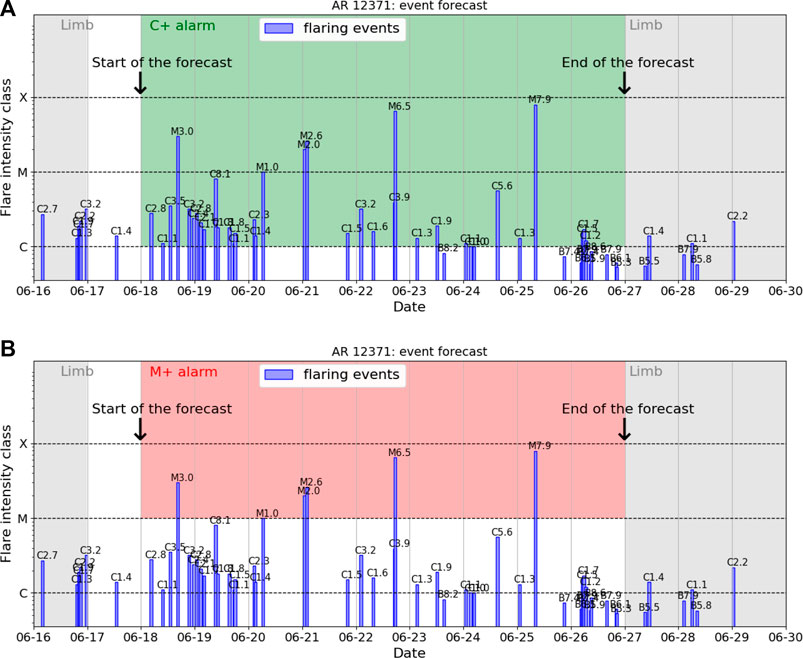
FIGURE 2. Predictions enrolled over time for the solar storm generated by AR 12371. The actual flaring events recorded by GOES, together with the corresponding GOES flare classes, are reported. The gray regions correspond to temporal windows out of the field of view of the HMI. (A) Warnings of C1+ flares are in green. (B) Warnings of M1+ flares are in red.

TABLE 7. Predictions of the solar storm associated to AR 12371. The first prediction was made on 18 June 2015, and the last one was on 26 June 2015.
Figure 3 shows the prediction enrolled over time associated to AR 12673. The first prediction is made on 31-08-2017 00:00 for the next 24 h and the last prediction is made on 09-09-2017 for the next 24 h, since after that date, the AR was out from the field of view of the HMI. The samples to predict are 2 X-, 4 M-, 1 C-, and 3 NO2-class samples. The first 3 NO2-class samples are correctly predicted as negative samples. The algorithm correctly sent warnings of C1+ flares from 04-09-2017 to 20-03-2015, but it missed the C-class sample associated to the time range between 03-09-2017 00:00 UT and 03-09-2017 23:59 UT (the figure shows that this C-class sample is associated to the occurrence of a C1.1-class flare which has the peak time at 20:50). For the prediction of M1+ flares, the algorithm missed the first M-class sample associated to the time range between 04-08-09-2017 00:00 and 04-09-2017 23:59 UT, and then from 05-09-2017 00:00 UT, it correctly sent warnings until 10-09-2017. In Table 8, the confusion matrices are reported for the C1+ and M1+ flare predictions.
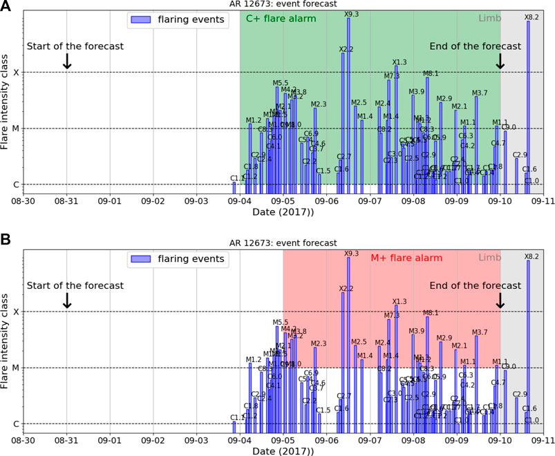
FIGURE 3. Predictions enrolled over time for the solar storm generated by AR 12673. The actual flaring events recorded by GOES, together with the corresponding GOES flare classes, are reported. The gray regions correspond to temporal windows out of the field of view of the HMI. (A) Warnings of C1+ flares are in green. (B) Warnings of M1+ flares are in red.

TABLE 8. Predictions of the solar storm associated to AR 12673. The first prediction was made on 30 August 2017, and the last one was on 9 September 2017.
4 Conclusion
This study shows that the video-based deep learning strategy for flare forecasting introduced in Guastavino et al. (2022a) can be exploited in an operational setting. This approach populates the training and validation sets for supervised algorithm accounting for the rates of the flare types associated to the specific temporal window of the solar cycle. The effectiveness of the proposed setting is proved by comparing the results obtained, considering both the same and a different solar phase with respect to the test window. The prediction algorithm is an LRCN that takes videos of line-of-sight magnetograms as input and provides a binary prediction of the flare occurrence as output. The innovative flavor of this approach is strengthened by the use of SOL functions in the optimization step and of value-weighted skill scores in the validation and test phases. Moreover, the results concerning the three solar storms show that this approach can be used as an operational warning machine for flare forecasting on a daily scale. As far as future work is concerned, the proposed approach for the construction of training and validation data sets may be further improved by taking into account additional features, trends, and recurrences that affect the behavior of solar cycles on an extended timescale.
Data availability statement
The data used for this study named Space-weather HMI Active Region Patches (SHARP) Bobra et al. (2014) are provided by the SDO/HMI team, publicly available at the Joint Science Operations Center. They can be found at the following software repository https://github.com/mbobra/SHARPs.
Author contributions
SG and FM worked on the implementation of the computational strategy. MP, FB, and CC contributed to the formulation of the method and the design of the experiments. SG, FM, and MP drafted the manuscript. All authors collaborated in conceiving the general scientific ideas at the basis of the study.
Funding
SG and FM acknowledge the financial support of the Programma Operativo Nazionale (PON) “Ricerca e Innovazione” 2014–2020. This research was made possible by the financial support from the agreement ASI-INAF n.2018-16-HH.0.
Acknowledgments
The authors enjoyed fruitful discussions with Dr. Manolis Georgoulis, who is kindly acknowledged.
Conflict of interest
The authors declare that the research was conducted in the absence of any commercial or financial relationships that could be construed as a potential conflict of interest.
Publisher’s note
All claims expressed in this article are solely those of the authors and do not necessarily represent those of their affiliated organizations, or those of the publisher, editors, and reviewers. Any product that may be evaluated in this article, or claim that may be made by its manufacturer, is not guaranteed or endorsed by the publisher.
References
Aschwanden, M. J. (2008). Keynote address: Outstanding problems in solar physics. J. Astrophys. Astron. 29, 3–16. doi:10.1007/s12036-008-0002-5
Astafyeva, E., Zakharenkova, I., and Förster, M. (2015). Ionospheric response to the 2015 st. patrick’s day storm: A global multi-instrumental overview. J. Geophys. Res. Space Phys. 120, 9023–9037. doi:10.1002/2015ja021629
Barnes, G., Leka, K. D., Schrijver, C. J., Colak, T., Qahwaji, R., Ashamari, O. W., et al. (2016). A comparison of flare forecasting methods. I. Results from the “all-clear” workshop. Astrophys. J. 829, 89. doi:10.3847/0004-637x/829/2/89
Benvenuto, F., Campi, C., Massone, A. M., and Piana, M. (2020). Machine learning as a flaring storm warning machine: Was a warning machine for the 2017 september solar flaring storm possible? Astrophysical J. Lett. 904, L7. doi:10.3847/2041-8213/abc5b7
Bloomfield, D. S., Higgins, P. A., McAteer, R. J., and Gallagher, P. T. (2012). Toward reliable benchmarking of solar flare forecasting methods. Astrophys. J. 747, L41. doi:10.1088/2041-8205/747/2/l41
Bobra, M. G., and Couvidat, S. (2015). Solar flare prediction using sdo/hmi vector magnetic field data with a machine-learning algorithm. Astrophys. J. 798, 135. doi:10.1088/0004-637x/798/2/135
Bobra, M. G., Sun, X., Hoeksema, J. T., Turmon, M., Liu, Y., Hayashi, K., et al. (2014). The helioseismic and magnetic imager (hmi) vector magnetic field pipeline: Sharps–space-weather hmi active region patches. Sol. Phys. 289, 3549–3578. doi:10.1007/s11207-014-0529-3
Campi, C., Benvenuto, F., Massone, A. M., Bloomfield, D. S., Georgoulis, M. K., and Piana, M. (2019). Feature ranking of active region source properties in solar flare forecasting and the uncompromised stochasticity of flare occurrence. Astrophys. J. 883, 150. doi:10.3847/1538-4357/ab3c26
Crown, M. D. (2012). Validation of the noaa space weather prediction center’s solar flare forecasting look-up table and forecaster-issued probabilities. Space weather. 10. doi:10.1029/2011sw000760
Donahue, J., Hendricks, L. A., Rohrbach, M., Venugopalan, S., Guadarrama, S., Saenko, K., et al. (2017). Long-term recurrent convolutional networks for visual recognition and description. IEEE Trans. Pattern Anal. Mach. Intell. 39, 677–691. doi:10.1109/TPAMI.2016.2599174
Florios, K., Kontogiannis, I., Park, S.-H., Guerra, J. A., Benvenuto, F., Bloomfield, D. S., et al. (2018). Forecasting solar flares using magnetogram-based predictors and machine learning. Sol. Phys. 293, 28–42. doi:10.1007/s11207-018-1250-4
Georgoulis, M. K., Bloomfield, D. S., Piana, M., Massone, A. M., Soldati, M., Gallagher, P. T., et al. (2021). The flare likelihood and region eruption forecasting (FLARECAST) project: Flare forecasting in the big data & machine learning era. J. Space Weather Space Clim. 11, 39. doi:10.1051/swsc/2021023
Guastavino, S., Marchetti, F., Benvenuto, F., Campi, C., and Piana, M. (2022a). Implementation paradigm for supervised flare forecasting studies: A deep learning application with video data. Astron. Astrophys. 662, A105. doi:10.1051/0004-6361/202243617
Guastavino, S., Piana, M., and Benvenuto, F. (2022b). Bad and good errors: Value-weighted skill scores in deep ensemble learning. IEEE Trans. Neural Netw. Learn. Syst., 1–10. doi:10.1109/tnnls.2022.3186068
Guastavino, S., Piana, M., Massone, A. M., Schwartz, R., and Benvenuto, F. (2019). Desaturating sdo/aia observations of solar flaring storms. Astrophys. J. 882, 109. doi:10.3847/1538-4357/ab35d8
Guastavino, S., Piana, M., Tizzi, M., Cassola, F., Iengo, A., Sacchetti, D., et al. (2021). Prediction of severe thunderstorm events with ensemble deep learning and radar data.
Hochreiter, S., and Schmidhuber, J. (1997). Long short-term memory. Neural Comput. 9, 1735–1780. doi:10.1162/neco.1997.9.8.1735
Hu, A., Shneider, C., Tiwari, A., and Camporeale, E. (2022). Probabilistic prediction of dst storms one-day-ahead using full-disk soho images. Space weather.
Huang, X., Wang, H., Xu, L., Liu, J., Li, R., and Dai, X. (2018). Deep learning based solar flare forecasting model. i. results for line-of-sight magnetograms. Astrophys. J. 856, 7. doi:10.3847/1538-4357/aaae00
Joshi, B., Ibrahim, M. S., Shanmugaraju, A., and Chakrabarty, D. (2018). A major geoeffective cme from noaa 12371: Initiation, cme–cme interactions, and interplanetary consequences. Sol. Phys. 293, 107–120. doi:10.1007/s11207-018-1325-2
Kingma, D. P., and Ba, J. (2015). “Adam: A method for stochastic optimization,” in 3rd International Conference on Learning Representations, ICLR 2015, San Diego, CA, USA, May 7-9, 2015. Editors Y. Bengio, and Y. LeCun
Li, X., Zheng, Y., Wang, X., and Wang, L. (2020). Predicting solar flares using a novel deep convolutional neural network. Astrophys. J. 891, 10. doi:10.3847/1538-4357/ab6d04
Liu, C., Deng, N., Wang, J. T., and Wang, H. (2017). Predicting solar flares using sdo/hmi vector magnetic data products and the random forest algorithm. Astrophys. J. 843, 104. doi:10.3847/1538-4357/aa789b
Liu, H., Liu, C., Wang, J. T., and Wang, H. (2019). Predicting solar flares using a long short-term memory network. Astrophys. J. 877, 121. doi:10.3847/1538-4357/ab1b3c
Marchetti, F., Guastavino, S., Piana, M., and Campi, C. (2022). Score-oriented loss (SOL) functions. Pattern Recognit. 132, 108913. doi:10.1016/j.patcog.2022.108913
Mason, J. P., and Hoeksema, J. T. (2010). Testing automated solar flare forecasting with 13 years of michelson Doppler imager magnetograms. Astrophys. J. 723, 634–640. doi:10.1088/0004-637X/723/1/634
McAteer, R. T. J., Gallagher, P. T., and Conlon, P. A. (2010). Turbulence, complexity, and solar flares. Adv. Space Res. 45, 1067–1074. doi:10.1016/j.asr.2009.08.026
Murray, S. A., Bingham, S., Sharpe, M., and Jackson, D. R. (2017). Flare forecasting at the met office space weather operations centre. Space weather. 15, 577–588. doi:10.1002/2016sw001579
Nayak, C., Tsai, L.-C., Su, S.-Y., Galkin, I., Tan, A. T. K., Nofri, E., et al. (2016). Peculiar features of the low-latitude and midlatitude ionospheric response to the st. patrick’s day geomagnetic storm of 17 march 2015. J. Geophys. Res. Space Phys. 121, 7941–7960. doi:10.1002/2016ja022489
Nishizuka, N., Kubo, Y., Sugiura, K., Den, M., and Ishii, M. (2021). Operational solar flare prediction model using Deep Flare Net. Earth Planets Space 73, 64. doi:10.1186/s40623-021-01381-9
Nishizuka, N., Kubo, Y., Sugiura, K., Den, M., and Ishii, M. (2020). Reliable probability forecast of solar flares: Deep flare net-reliable (DeFN-R). Astrophys. J. 899, 150. doi:10.3847/1538-4357/aba2f2
Nishizuka, N., Sugiura, K., Kubo, Y., Den, M., and Ishii, M. (2018). Deep flare net (defn) model for solar flare prediction. Astrophys. J. 858, 113. doi:10.3847/1538-4357/aab9a7
Pandey, C., Ji, A., Angryk, R. A., Georgoulis, M. K., and Aydin, B. (2022). Towards coupling full-disk and active region-based flare prediction for operational space weather forecasting. Front. Astron. Space Sci. 9, 897301. doi:10.3389/fspas.2022.897301
Pesnell, W. D., Thompson, B. J., and Chamberlin, P. (2011). “The solar dynamics observatory (sdo),” in The solar dynamics observatory (Berlin: Springer), 3–15.
Petrakou, E. (2018). A deterministic model for forecasting long-term solar activity. J. Atmos. Solar-Terrestrial Phys. 175, 18–23. doi:10.1016/j.jastp.2018.04.009
Qian, L., Wang, W., Burns, A. G., Chamberlin, P. C., Coster, A., Zhang, S.-R., et al. (2019). Solar flare and geomagnetic storm effects on the thermosphere and ionosphere during 6–11 september 2017. JGR. Space Phys. 124, 2298–2311. doi:10.1029/2018ja026175
Rosasco, L., De Vito, E., Caponnetto, A., Piana, M., and Verri, A. (2004). Are loss functions all the same? Neural Comput. 16, 1063–1076. doi:10.1162/089976604773135104
Scherrer, P. H., Schou, J., Bush, R., Kosovichev, A., Bogart, R., Hoeksema, J., et al. (2012). The helioseismic and magnetic imager (hmi) investigation for the solar dynamics observatory (sdo). Sol. Phys. 275, 207–227. doi:10.1007/s11207-011-9834-2
Schwenn, R. (2006). Space weather: The solar perspective. Living Rev. Sol. Phys. 3, 1–72. doi:10.12942/lrsp-2006-2
Shibata, K. (1996). New observational facts about solar flares from yohkoh studies—Evidence of magnetic reconnection and a unified model of flares. Adv. Space Res. 17, 9–18. doi:10.1016/0273-1177(95)00534-l
Song, H., Tan, C., Jing, J., Wang, H., Yurchyshyn, V., and Abramenko, V. (2009). Statistical assessment of photospheric magnetic features in imminent solar flare predictions. Sol. Phys. 254, 101–125. doi:10.1007/s11207-008-9288-3
Strugarek, A., and Charbonneau, P. (2014). Predictive capabilities of avalanche models for solar flares. Sol. Phys. 289, 4137–4150. doi:10.1007/s11207-014-0570-2
Su, Y., Veronig, A. M., Holman, G. D., Dennis, B. R., Wang, T., Temmer, M., et al. (2013). Imaging coronal magnetic-field reconnection in a solar flare. Nat. Phys. 9, 489–493. doi:10.1038/nphys2675
Sui, L., Holman, G. D., and Dennis, B. R. (2004). Evidence for magnetic reconnection in three homologous solar flares observed by rhessi. Astrophys. J. 612, 546–556. doi:10.1086/422515
Sun, Z., Bobra, M. G., Wang, X., Wang, Y., Sun, H., Gombosi, T., et al. (2022). Predicting solar flares using CNN and LSTM on two solar cycles of active region data. Astrophys. J. 931, 163. doi:10.3847/1538-4357/ac64a6
Vemareddy, P. (2017). Successive homologous coronal mass ejections driven by shearing and converging motions in solar active region noaa 12371. Astrophys. J. 845, 59. doi:10.3847/1538-4357/aa7ff4
Keywords: solar flares, deep learning, evaluation metrics, operational forecasting, machine learning
Citation: Guastavino S, Marchetti F, Benvenuto F, Campi C and Piana M (2023) Operational solar flare forecasting via video-based deep learning. Front. Astron. Space Sci. 9:1039805. doi: 10.3389/fspas.2022.1039805
Received: 08 September 2022; Accepted: 21 November 2022;
Published: 07 March 2023.
Edited by:
Enrico Camporeale, University of Colorado Boulder, United StatesReviewed by:
Alexey A. Kuznetsov, Institute of Solar-Terrestrial Physics (RAS), RussiaP. Vemareddy, Indian Institute of Astrophysics, India
Copyright © 2023 Guastavino, Marchetti, Benvenuto, Campi and Piana. This is an open-access article distributed under the terms of the Creative Commons Attribution License (CC BY). The use, distribution or reproduction in other forums is permitted, provided the original author(s) and the copyright owner(s) are credited and that the original publication in this journal is cited, in accordance with accepted academic practice. No use, distribution or reproduction is permitted which does not comply with these terms.
*Correspondence: Sabrina Guastavino, Z3Vhc3Rhdmlub0BkaW1hLnVuaWdlLml0