Ionospheric response modeling under eclipse conditions: Evaluation of 14 December 2020, total solar eclipse prediction over the South American sector

1 Introduction

Among the multiple phenomena that impact and modify the ionosphere state, solar eclipses have been extensively studied thanks to the high predictive accuracy of the solar irradiation reduction and its posterior increase generated by the Moon blockage (Beynon, 1955; Rishbeth, 1968; Jose et al., 2020). Early studies prior to the discovery of the ionosphere already suggested that the origin of the ionization of the upper atmospheric layers is solar radiation (Rishbeth, 1968). Indeed, solar EUV and X-ray emissions are some of the main sources of ionospheric plasma. In addition, variations of solar irradiance, in their multiple scales (i.e., daily, seasonal, and solar periods) and in particular space weather events (e.g., solar flares), directly impact the ionospheric formation and dynamics. Therefore, the irradiation reduction generated by the solar obscuration greatly impacts the ionization of the different layers of the ionosphere (e.g., Beynon, 1955; Rishbeth, 1968; Goncharenko et al., 2018). For this reason, eclipses have long been considered large-scale ionospheric experiments and their effects have been measured using multiple instruments, providing extremely relevant information on the characteristics of the different layers of the ionosphere (for a detailed review of the historical usage of eclipses to study the ionosphere see Appendix A of Bravo et al., 2020).

Nevertheless, the Sun is a non-uniform source of ionization and the ionosphere does not behave as a perfect irradiation detector (Rishbeth, 1968). Hence, the different layers of the ionosphere suffer different effects during the eclipse obscuration. The lower ionosphere (E and F1 layers) presents large density depletions due to the predominance of recombination among photoionization processes at these altitudes. Moreover, during the eclipse totality, coronal emissions are not completely blocked by the Moon, providing approximately 2% of the total solar photoionization rate which generates ionization at altitudes below 200 km, mainly impacting the production of the F1 layer (Reinisch et al., 2018). On the other hand, a large diversity of eclipse impacts have been reported at higher altitudes (i.e., F2 layer). At these altitudes, diffusion and transport plasma processes generally dominate the ionospheric behavior, making the ionospheric response to the eclipse highly dependent on different latitudinal effects (Le et al., 2009). In particular, multiple studies have demonstrated that the ionospheric response to eclipses at equatorial and low latitudes is dominated by the fountain effect and the Equatorial Ionization Anomaly (EIA; e.g., Martínez-Ledesma et al., 2020; Bravo et al., 2020; Jonah et al., 2020; Jose et al., 2020; Adekoya & Chukwuma, 2016; Cheng et al., 1992; Le et al., 2009). Furthermore, the multiple coupling processes that interact in the magnetosphere-ionosphere-thermosphere system and the internal ionospheric processes provide large variability to the ionospheric state (Sarris, 2019). These different interactions and processes interplay between them during an eclipse and generate a large diversity of possible response scenarios, being particularly challenging to accurately determine the ionospheric impacts of eclipses at equatorial and low latitudes. Then, not only multiple instrumental measurements are required to study and identify the different eclipse impacts on the ionosphere, but also ionospheric models with an accurate representation of the different processes occurring at these latitudes are needed. More significantly, the direct comparison of simulations and measurements of the ionospheric response to eclipses can be used as a testbed of the ionospheric model reproducibility, helping quantify the accuracy of the simulation results and also our state of knowledge in the physics of the different ionospheric processes observed.

In this study, the ionospheric response to the 14 December 2020, solar eclipse measured over South America is compared to the SUPIM-INPE model prediction made by Martínez-Ledesma et al. (2020). Here, we evaluate the response along the South-American continent, covering a wide range of geomagnetic latitudes, from the Equator (e.g., Jicamarca) to mid-latitude sectors (e.g., Bahía Blanca). Measurements of multiple ground-based instruments along the continent (i.e., ionosonde stations, an Incoherent Scatter Radar, and GNSS receiver networks) and satellites (i.e., Swarm-A) are used to evaluate the accuracy of simulation results, providing a testbed scenario to determine the accuracy of the ionospheric prediction model under total eclipse conditions. In addition, the results of this evaluation are compared to the ionospheric response to the 2 July 2019, solar eclipse that occurred in the same geographical area (Bravo et al., 2020; Jonah et al., 2020; Maurya et al., 2020) and previous studies that evaluated the ionospheric response to the 14 December 2020, solar eclipse (e.g., Gómez, 2021; Meza et al., 2021; Shrivastava et al., 2021; de Haro Barbás et al., 2022; Resende et al., 2022).

2 Materials and methods

2.1 Ionospheric model

The prediction of the ionospheric impact of the 14 December 2020, eclipse done by Martínez-Ledesma et al. (2020) was determined using the Sheffield University Plasmasphere Ionosphere Model (Bailey & Sellek, 1990; Bailey et al., 1993) adapted at the Instituto Nacional de Pesquisas Espaciais, under the name SUPIM-INPE (Souza et al., 2010, 2013; Santos et al., 2016). In SUPIM, time-dependent equations of continuity, momentum, and energy balance that describe the chemical and physical processes of the Earth’s mid-and low-latitude ionosphere and plasmasphere, are solved along closed dipole magnetic field lines from altitudes of 90 km in conjugate hemispheres to give values for the densities, field-aligned velocities, and temperatures of the O+, H+, He+, N2+, O2+, NO+, N+ ions, and electrons.

The principal chemical and physical processes considered within the model include ion production due to solar EUV radiation, ion production and loss due to chemical reactions between the constituent ions and with the neutral gasses, ambipolar and thermal diffusion, ion-ion and ion-neutral collisions, thermospheric winds, electrodynamic drift, thermal conduction, photoelectron heating, frictional heating, and a host of local heating and cooling mechanisms (Bailey et al., 1997).

SUPIM-INPE uses geomagnetic coordinates of the International Geomagnetic Reference Field (IGRF 13th Generation); the neutral densities from the NRLMSISE-00 model (Picone et al., 2002); the neutral wind from HWM93 model (Hedin et al., 1996); the E x B vertical drift from Jicamarca Incoherent Scatter Radar measurements, or from the model of Fejer et al. (2008) in the absence of these; and the EUV irradiances from the model of Richards et al. (2010) based on the Solar EUV Experiment (SEE) measurements (Woods et al., 2005) for wavelengths greater than 27 nm and from the HEUVAC model (Richards et al., 2006) for wavelengths smaller than 27 nm.

In the case of the eclipse prediction of Martínez-Ledesma et al. (2020), SUPIM-INPE was modified to model the solar obscuration effect on the ionosphere, in low and middle magnetic latitudes. To do so, the solar input radiation (I_R) of the model during the eclipse for a given wavelength (λ) was assumed as

$I_R=I_{NT}+I_{R0}^{\lambda <30.4}\left(1-0.7\times ObsMask\right)+I_{R0}^{\lambda ⩾30.4}\left(1-ObsMask\right)(1)$

where I_NT is the nighttime radiation, I_R0^λ<30.4 and I_R0^{λ≥ 30.4} are the ionizing radiations for λ < 30.4 nm (coronal range) and λ ≥ 30.4 nm (chromospherical range), respectively, and ObscMask is the normalized value of the obscuration mask. In this study, the authors assumed that during the eclipse totality, a 30% of the coronal radiation remains, similarly as in previous studies (Reinisch et al., 2018; Bravo et al., 2020).

Although a C4-class solar flare was detected on the day of the eclipse, no significant ionospheric impact was observed during this day, as indicated in previous studies of this event (Gómez, 2021; de Haro Barbás et al., 2022). Therefore, in this study, we consider that no significant contribution modified the overall ionospheric response to the eclipse, allowing a direct comparison to the model prediction results. In addition, the geomagnetic conditions during the day of the eclipse are quiet, presenting a daily index Ap = 3, with a maximum Kp index of 2^-.

2.2 Measurement instruments

Regarding the data used for the model validation, the following ionospheric stations were analyzed: Jicamarca (12.0° S, 76.8° W), Tucumán (26.9° S, 65.4° W), Chillán (36.6° S, 72.0° W) and Bahía Blanca (38.7° S, 62.3° W). Figure 1 shows the geographical location of these stations. Jicamarca and Tucumán stations barely reached 17% and 49% obscuration percentages at 300 km height during the eclipse, respectively. Alternatively, both Chillan and Bahía Blanca stations reached 95% and their measurements were previously analyzed in a recent study by de Haro Barbás et al. (2022). Jicamarca’s ionograms are obtained from a Digital Ionospheric Goniometric Ionosonde (DIGISONDE, https://www.digisonde.com) and are available in the Digital Ionogram Data Base (DIDBase), Global Ionosphere Radio Observatory (GIRO, https://giro.uml.edu).

FIGURE 1

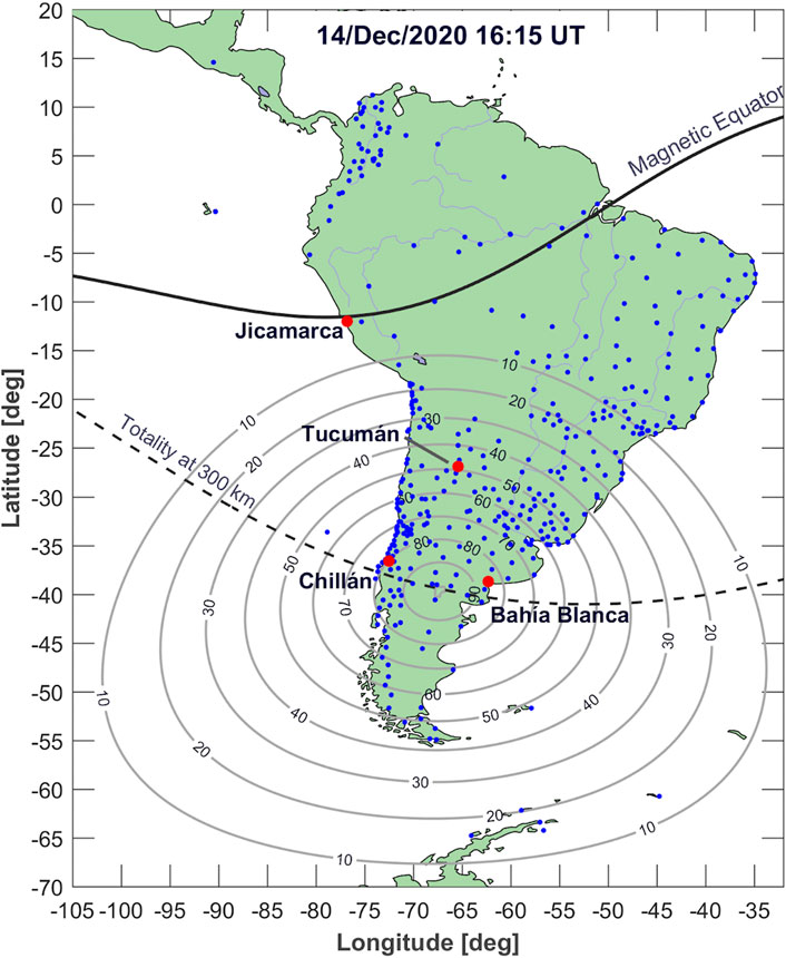
FIGURE 1. Geographical locations of the ionosondes (red circles), GNSS receivers (blue dots), and eclipse obscuration mask at 300 km height at 16.12 UT (continuous gray curves). Totality path at 300 km (dashed gray line).

Tucumán (low latitude) and Bahía Blanca (mid-latitude) stations have ionospheric sounders with similar AIS-INGV systems (Zuccheretti et al., 2003). Both stations are operated by the Tucumán Space Weather Center (https://spaceweather.facet.unt.edu.ar/), a research program of Facultad de Ciencias Exactas y Tecnología (FACET), Universidad Nacional de Tucumán, (UNT) Tucumán, Argentina. In these instruments, the vertical sounding technique is used to estimate the virtual height in the ionosphere, using a frequency ranging between 2 and 20 MHz. Both systems are usually configured to perform a complete sounding with a 10 min resolution, obtaining the so-called ionograms (Zuccheretti et al., 2003; Molina et al., 2013). Additionally, each ionogram is automatically scaled using the Autoscala software (Pezzopane et al., 2010) to obtain different ionospheric parameters such as foF2 or foF1, among others. Nevertheless, the foE parameter is not obtained automatically, therefore, it is necessary to do it manually. In the case of foF1 and foF2, in addition to the automatic result, it is often corrected manually to improve the data quality. In particular for this eclipse measurement campaign, both stations were configured with a sounding resolution of 5 min with the aim of capturing rapid changes in the ionospheric layers due to the eclipse path and also a manual validation was performed.

The Chillán station in Chile has an ionosonde from the Australian Ionospheric Prediction Service (IPS-42) produced by KEL Aerospace Pty Ltd. in 1979 (Wilkinson et al., 2018). Currently it is operated by the Centro Interuniversitario de Física de la Alta Atmósfera (Interuniversity Center for High Atmosphere Physics, CInFAA in Spanish). Previously, it was located at La Serena station (29.9° S, 71.3° W) where it was operational for the study of the solar eclipse that occurred on 2 July 2019 (Bravo et al., 2020) and was later transferred to the Universidad Adventista of Chile (UnACh). The ionograms of this ionosonde were processed manually using the Digital Ionogram Scaling Software (DISS; Urra, 2019), which also includes the POLAN software for estimating the full profile of electron density (Titheridge, 1985). In this software, the electron density values over the peak of maximum density (hmF2) are modeled based on the assumption of a constant scale height and shaped by an ɑ-Chapman function (Huang & Reinisch, 2001).

Additionally, measurements were done using the Jicamarca Incoherent Scatter Radar (ISR). This instrument is a phased array antenna of 288 m × 288 m formed by 18432 elements located in the Jicamarca Radio Observatory (JRO; 12.0° S, 76.8° W), Perú which operates by emitting high-power pulses of high-frequency signals (49.92 MHz) that traverse the ionosphere (Bowles et al., 1962). Faint backscatter signals generated by the Thompson scatter effect on the free electrons are received as echo responses to each pulse emission at different altitudes. The received signal intensity depends on the concentration of electrons, providing an initial estimate of the electron density profile that can reach ranges well above the maximum density peak altitude (hmF2). In addition, the frequency response of the backscatter signal provides information on the line-of-sight ion drift velocities (due to the Doppler effect) and the temperature of the ions and electrons present (Evans, 1969). The multi-parameter estimation capability of this instrument makes it of extreme relevance for understanding the overall dynamics of the ionospheric profile at the magnetic equator.

We also analyzed Total Electron Content (TEC), derived from Global Navigation Satellite System (GNSS) receivers. We used receivers available in the Chilean network set up by the National Seismological Center (CSN in Spanish, www.sismologia.cl), in the International GNSS Service network (IGS, www.igs.org; Dow et al., 2009), in the Low-Latitude Ionospheric Sensor Network (LISN, http://lisn.igp.gob.pe/), in the Argentine network (RAMSAC, www.ign.gob.ar; Piñón et al., 2018), in the Brazilian network (RBMC, ww2. ibge.gov.br), in the Uruguayan network (REGNA, ftp://pp.igm.gub.uy), and the Colombian network (MAGNA, https://geoportal.igac.gov.co). The sizable composite receiver network is shown in Figure 1 as blue dots.

Measurements of the Swarm mission of the European Space Agency (Friis-Christensen et al., 2008) were also evaluated. This mission contains three identical satellites in an approximately circular orbit of inclination of 87.75°. Swarm satellites are equipped with Langmuir probes on the Electric Field Instrument (EFI) to study the plasma environment around Earth (Knudsen et al., 2017). In situ data of the satellite Swarm-Alpha (A), which orbits the Earth at altitudes about 450 km, was evaluated to determine the eclipse impacts at high altitudes (https://earth.esa.int/web/guest/swarm/data-access, last accessed on 29 July 2022).

2.3 Data analysis

For each ionospheric station measurement, a reference curve was obtained as the average variation of the 5 geomagnetically quietest days of the interval measured by the stations simultaneously (04–17 of December 2020), as done in de Haro Barbás et al. (2022). The five quietest days selected are 04, 17, 07, 15, and 16 of December, sorted by calmest. These days present daily index Ap ≤ 2, with a maximum kp of 1⁺. It is worth mentioning that the five quietest days strategy to estimate the reference curve has been selected due to data availability at each of the stations and to avoid large data gaps when other periods are considered.

A measurement campaign was specifically carried out by the Jicamarca ISR to capture the eclipse and its impacts between the dates of 10th to 16th of December. Therefore, only these measurement days for which data were available have been considered as the reference curve. To accurately describe the eclipse induced effects measured by the ISR, only the electron density (N) data with estimated errors smaller than 7×10¹⁰ m⁻³, and electron and ion temperatures (Te and Ti, respectively) with estimated error smaller than 250 K were selected to be analysed. Furthermore, both the reference and eclipse-day data were filtered by using a temporal second-order Savitzky-Golay smoothing filter with a 2-h timeframe to eliminate non-eclipse related variabilities and the possible influence of Traveling Ionospheric Disturbances, TIDs (similarly as in the 21 August 2017 eclipse analysis of the Millstone Hill ISR made by Goncharenko et al., 2018).

It is a well known fact that different techniques for retrieving TEC from GNSS data obtain different TEC estimates (Pignalberi et al., 2021). Therefore, to provide a much more complete representation of the ionospheric impacts of the eclipse, we compared three different TEC analysis techniques. In these techniques, only TEC values corresponding to satellite elevation angles ≥15° were selected to minimize possible errors. In the same way as for the parameters of the ionosonde, the reference value is considered to be the median of 5 geomagnetically quietest days (similarly as in de Haro Barbás et al., 2022). Additionally, the data has been averaged between 2° of latitude and 2° of longitude over a 5 min time interval.

In a first instance, GPS-TEC analysis software version 2.9.5 (Seemala and Valladares, 2011; http://seemala.blogspot.com/) was used. This software calculates the slant TEC (sTEC) from pseudorange measurements from Receiver Independent Exchange Format (RINEX) files of each GPS receiver. The clock errors and tropospheric effects are minimized using the phase and code values for the transmitted L1 and L2 GPS frequencies. Differential satellite biases and receiver bias are included in determining the absolute values of sTEC. In the calculation of vertical TEC (vTEC) from sTEC, the satellite elevation and azimuth angles are used.

Another code used is PYTEC (https://github.com/sylvathle/PYTEC). Similarly as does the previous code, PYTEC computes the TEC from the dual frequencies of GPS satellites stored in RINEX format. This code is intended to respond to the need of an open-source code that calculates the TEC among the scientific community. This is the reason why PYTEC is implemented in Python and is expected to be encoded as a python module in future versions. In its current state, it uses satellites from the GPS constellation and requires the bias of the satellite clock as input. Following the method proposed by (Arikan et al., 2008), the bias of the receiver clock is compensated by minimizing the standard deviation of the sTEC time series available during 1 day obtained from all the satellites that could be reached. Also, an algorithm reconstructs most cycle-slips found in the signal.

Finally, GNSS RINEX files obtained at each station from GPS and GLONASS constellations were calibrated using the so-called Ciraolo method (Ciraolo et al., 2007). This technique derives TEC from carrier phase measurements for both GPS or GPS + GLONASS satellite systems. The ionospheric delay from the raw carrier phase observations can be modeled as the slant TEC (sTEC) plus the arc-offset. The contribution of each receiver and satellite biases and the contribution of any non-zero averaged errors over an arc of observation are considered. After obtaining the sTEC, the vTEC is estimated considering a two-dimensional thin shell model at 350 km. This method has been chosen due to its ability of calibrating GPS and GLONASS observations providing better resolution at each station.

To compare the eclipse impacts on the in situ electron density and temperature measurements made by the Swarm-A Lagmuir probes, the data evaluated has been obtained from the eclipse day and the geomagnetically quiet days previously selected. Additionally, due to the possible disparity of ionospheric perturbations observed at different geographic locations and times, we have chosen the seven Swarm satellite orbit transects that best fit the eclipse region and eclipse time window. Therefore, the comparison of the latitudinal density and temperature profiles of the day of the eclipse have been done with the two closest trajectories to the eclipse longitudinally and temporally. The trajectories selected on the 4th and 16th of December have differences of ∼7° of longitude over the geographic equator and ∼10 min.

2.4 Model-measurement comparison method

With the purpose of evaluating the performance of the model, a comparative statistical analysis was done calculating both the Pearson (r) and the Spearman (ρ) correlation coefficients with a confidence level of 95% between the prediction of SUPIM-INPE and measured values. The Pearson correlation coefficient evaluates the linear association between two continuous variables normally distributed. On the other hand, the Spearman correlation coefficient allows us to evaluate monotonic relationships between variables that do not require to be normally distributed. Moreover, the Spearman coefficient is more robust to possible data outliers. The comparison of the two coefficients provides a more robust indication of the correlation relationship between the model prediction and the measured data. Additionally, as the correlation only speaks of the similarity of the two time series, the normalized root-mean-square error (NRMSE) has been calculated to provide a direct comparison of the accuracy of the model prediction. The mathematical expression of the NRMSE used (normalized by the mean value of the measurements) is given by:

$NRMSE\left(\%\right)=100\frac{\sqrt{\frac{\sum _{i=1}^n{\left|x_i-m_i\right|}^2}{n}}}{\frac{\sum _{i=1}^n{x}_i}{n}}(2)$

where x_i and m_i are the measured and modeled values, respectively.

The study of Chukwuma & Adekoya (2016) has already used together both r and RMSE to evaluate the ionospheric response to the 20 March 2015 solar eclipse. Moreover, the study of Prietrella et al. (2016) used the RMSE metric to compare the performance of different ionospheric models in this same eclipse. Additionally, both the RMSE and NRMSE metrics are commonly used to evaluate ionospheric model studies (e.g., Araujo-Pradere & Fuller-Rowell, 2002; Matsuo & Araujo-Pradere, 2011; Pignalberi et al., 2021; Kosary et al., 2022).

Furthermore, to provide further statistical methods for the comparison of the empirical data to the modelled values, the two-sample Kolmogorov-Smirnov (K-S) test (Massey, 1951; Teegavarapu, 2019) and the two-sample Wilcoxon rank-sum (W) test (Gibbons & Chakraborti, 2011) are also evaluated. These two non-parametric methods provide a verification of the statistical distribution of the populations of the two time series by performing a null hypothesis testing analysis. The K-S test is a non-parametric hypothesis test that evaluates the difference between the cumulative distribution functions of the two datasets. Therefore, the verification of the null hypothesis of the K-S test indicates that both distributions are identical, independently on the type of statistical distribution of the data. Alternatively, the W-test has a null hypothesis that the medians of the two populations are identical. The median of the distribution could be directly compared to verify the accuracy of the prediction, although the distributions are found different by the K-S test. On the other hand, it is relevant to highlight that the real data measured may contain a larger variance than the predicted values due to measurement errors, instrumental resolution, internal (thermal) and external (sky) noise, interferences, and the additional ionospheric variability generated by thermosphere or magnetosphere interactions or internal modifications (e.g., gravity waves, etc.).

These metrics were calculated for the different parameters obtained from the ionosonde stations and for the TEC estimations calculated using the three techniques previously described. All the previously mentioned comparisons have been done for the entire daily variation (12 UT to 24 UT) and also for the eclipse obscuration time. The analysis of these two periods allows us to verify the correct model reproduction of both the daily variations at each station and their particular responses to the eclipse.

3 Results

3.1 Ionosonde parameters and TEC

The ionospheric critical frequency parameters (foF2, foF1, and foE) are shown in Figure 2 for each of the selected stations. This figure also represents the TEC calculated using the three different techniques previously indicated. Moreover, these parameters are compared to the SUPIM-INPE predicted values (gray lines) calculated in Martínez-Ledesma et al. (2020).

FIGURE 2

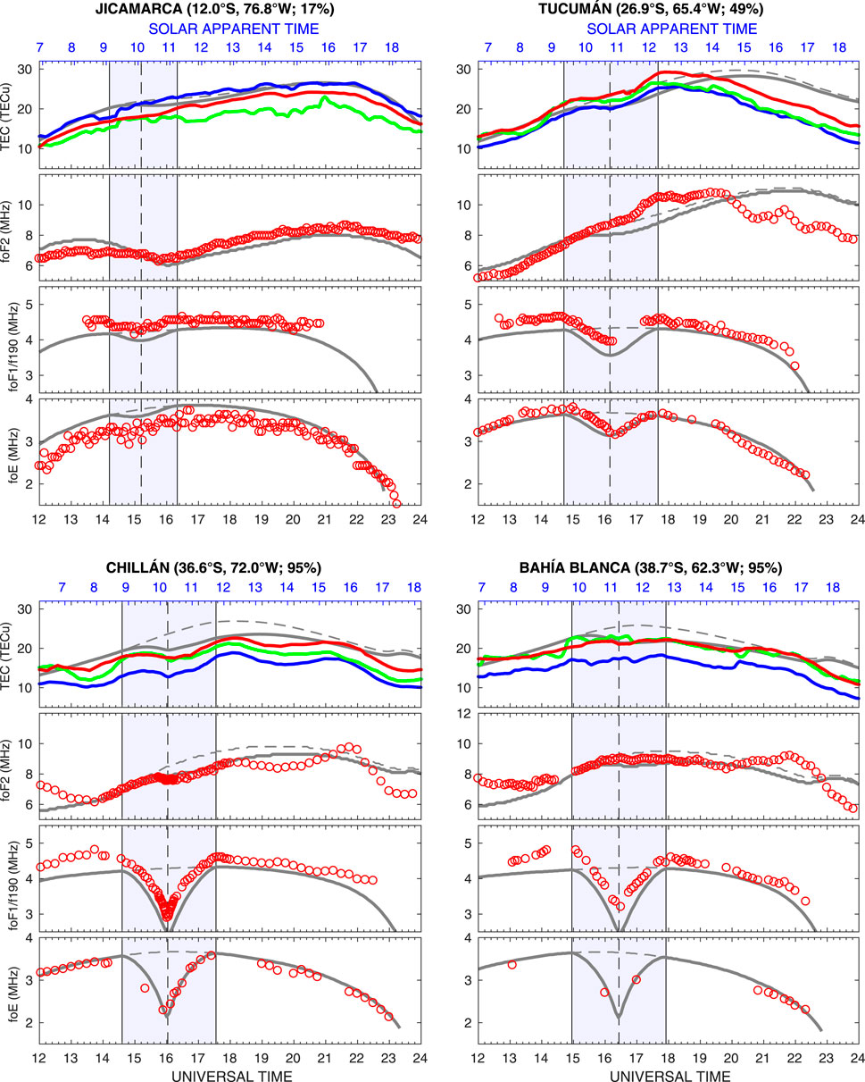
FIGURE 2. Comparison of SUPIM-INPE prediction simulations under reference (gray dashed lines) and eclipse (gray continuous lines) conditions for TEC, foF2, f190/foF1, and foE and observed data at different stations. TEC obtained from three different techniques (Seemala, PYTEC, and Ciraolo, in blue, green, and red continuous lines, respectively) and ionosonde observed parameters (red circles) are shown. Eclipse onset, maximum obscuration, eclipse end (shaded interval), and maximum percentages of obscuration are calculated at 300 km height.

In Jicamarca station, a good matching between the measured parameters and the model is observed, although we can observe only small variations during the eclipse time. Indeed, the effect of the eclipse is very weak, barely a deviation from the reference curve. The measured data shows a decrease in the values but, unlike the other stations, a marked peak is not observed at the moment of the maximum of the eclipse for that place. This is related to the low percentage of obscuration received at this location. On the other hand, the other three stations present much clear disturbances related to the eclipse.

In the case of E-layer, the foE shows a good matching between the observed and predicted values in Tucumán, Chillán, and Bahía Blanca, despite the low number of observations obtained in the latter station. Both, the model and the measured data, highly deviate from the reference values, as expected, showing the most significant decrease during the time of local maximum obscuration at each site. The model fits well for the Chillán and Tucumán stations, particularly in the recovery phase, after reaching the minimum, which coincides with the moment of maximum obscuration. But, at the beginning of the eclipse effect, the model in particular for the Chillán station overestimates (∼4%), while for the Tucumán station it underestimates (∼3%).

Analyzing the results of the F1-layer, we see that in the four stations the model presents values slightly lower than the measured values (<0.5 MHz). This deviation can be directly associated with the usage of an iso-height curve at 190 km in the modeled density profiles instead of a critical frequency. Even so, again at Tucumán, Chillán, and Bahía Blanca, there is a good correlation between the predicted curves and the observations. Maximum reduction values are all centered on the time of local maximum obscuration, except for the foF1 in Jicamarca which shows a slight deviation after its maximum obscuration time.

In the F2-layer case, the comparison requires a more detailed analysis. During the hours of the eclipse, both Chillán and Bahía Blanca stations show a good matching with the prediction. Indeed, these two stations are located at similar geographical latitudes and obtained a similar obscuration percentage (de Haro Barbás et al., 2022). After the eclipse hours (after 18 UT), the observations of Tucumán, Bahia Blanca and Chillán stations deviate from the predictions. Tucumán station shows a much larger deviation from the predicted values, particularly after the eclipse maximum obscuration. In particular, both Chillán and Bahía Blanca stations show a peak around 22 UT exceeding the prediction, while Tucumán obtains values much lower than the prediction after 20 UT. In this last case, the reason is likely that SUPIM-INPE is not able to reproduce some transport effects that may happen after eclipses in equatorial and mid-latitude regions (Zhang et al., 2010).

In the case of the TEC, the three techniques evaluated provide different results. The predictions are close to the TEC obtained using the Seemala’s technique (blue line) both in Jicamarca and Tucumán stations, but overestimates by ∼5 TECu in mid-latitudes (i.e., Chillán and Bahía Blanca stations). Alternatively, Tucumán and Bahía Blanca stations have similar values to the prediction when using the TEC obtained with the PYTEC technique (green line). Nevertheless, the predicted values at Jicamarca and Chillán overestimate the TEC determinations obtained using this technique (∼21% and ∼12% respectively). On the other hand, the Ciraolo technique (red line) has a good TEC matching in the mid-latitude stations, but it underestimates in Jicamarca (∼10%) and overestimates in Tucumán (∼13%). Therefore, the methods that provide the best matching to the predictions are PYTEC (except in Jicamarca) and Ciraolo’s methods. Regarding the overall behavior of TEC using different techniques, at the eclipse time any of the methods are able to follow the predicted trend. The more accentuated differences can be observed at the end of the day at Tucumán, Bahía Blanca, and Chillán.

3.2 Latitudinal TEC

The magnetic latitudinal response in TEC derived from GNSS receivers using the PYTEC code and its corresponding model prediction are shown in Figure 3. This figure shows the average TEC for quiet and eclipse conditions and their differences (ΔTEC) along the magnetic meridian of Chillán. In this figure, it can be seen a TEC reduction that occurs during the eclipse shadow traversing. Nevertheless, some negative values of ΔTEC are also observed before the event starts. This negative behavior stars around 13 UT and extends from −50° to 0° of magnetic latitude, having a slow recovery over time. In addition, a secondary and minor reduction is obtained almost simultaneously to the eclipse occurrence on the upper magnetic hemisphere (between 10° and 20° magnetic latitude). Indeed, this secondary reduction is consistent with the first conjugate decrease of the SUPIM-INPE prediction (occurring approximately between 17 UT and 20 UT). On the other hand, it is observed that the ΔTEC values are about double the predicted values. Additionally, it is relevant to note that TEC increases are observed between −50° and −30° after 17 UT (consistent with the foF2 observed at stations at these latitudes) and between -10° and 30° after 19 UT, being this second increase of much higher amplitude. For comparison, similar figures have been calculated using the other two TEC techniques and are provided in the Supplementary Material. The results in ΔTEC observed with these techniques present similar features to those obtained in Figure 3, but with some differences in the amplitudes.

FIGURE 3

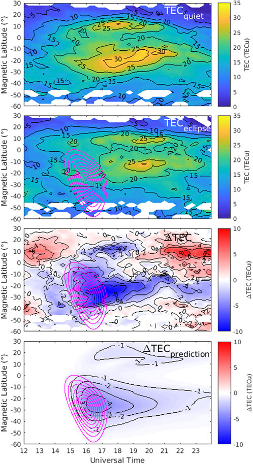
FIGURE 3. Total electron content response time evolution obtained with the PYTEC technique for reference day (top), the 14 December 2020, solar eclipse (middle), and eclipse-modified differences of TEC (ΔTEC, third row) along the magnetic meridian of Chillán (36.6°S, 72.0°W) and the SUPIM-INPE predicted differences (ΔTEC_prediction, bottom). Evolution of the eclipse obscuration mask at 300 km height each 10% obscuration (magenta lines).

3.3 Vertical distribution

Figure 4 shows the true height electron concentration profiles deduced from ionograms obtained at Chillán station (with 95% obscuration conditions). At altitudes below 200 km, there is a clear electron density reduction during the solar obscuration event and a subsequent recovery at the end of it. This density reduction and its posterior increase at low altitudes were expected by the prediction due to the predominance of photoionization processes at these heights. At the F2 region height (over 250 km), however, this decrease is delayed and persists in time until 21.75 UT, when the density peak is lower in height and higher in magnitude than the reference profiles (as shown in Figure 2). It is worth mentioning that, in this figure, as it previously indicated, density values are modeled over the hmF2 (red line) by the POLAN code. Therefore, the deviations shown above this peak height are subjected not only to possible ionospheric modifications of the upper profile but also are dependent on the quality of the measured profile and/or ionogram. For comparison, the fourth panel of Figure 4 shows the predicted deviation, which presents a decrease in electron concentration that clearly differs in its shape. The main difference to the prediction is found particularly at altitudes around 250 km, well above both E and F1 regions. Even so, at altitudes below 250 km, the predicted electron density decrease is close in magnitude to the measured profiles.

FIGURE 4

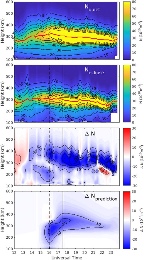
FIGURE 4. True height electron concentration profiles deduced from the ionograms of the reference day (top), eclipse day (middle), and eclipse-modified differences of the electron concentration (ΔN, third row) over time in Chillán (36.6°S, 72.0°W) and the SUPIM-INPE predicted differences (ΔN_prediction, bottom). The estimated peak height of the maximum electron concentration is presented (red line). Eclipse onset, maximum obscuration, and eclipse end (vertical lines) are calculated at 300 km height.

3.4 ISR of Jicamarca

The vertical distribution of electron concentration, along with electron and ion temperatures, measured by the Jicamarca ISR (with 17% obscuration conditions) are shown in Figure 5. In this figure, a large number of data gaps are obtained above the F2 peak (i.e., altitudes higher than ∼350 km) due to the filtering of the measurements with large estimation errors previously indicated. This increase in the measurement uncertainty is related to the low signal-to-noise-ratio obtained by the radar at high altitudes and during the maximum obscuration time, which is, in turn, due to the inverse relation of the received power to the distance squared, the fainter backscatter received from lower electron density areas, and the variation of the sky noise captured by the antenna. However, the general ionospheric trends are well represented in this figure, allowing us a direct comparison to the predicted values (bottom row).

FIGURE 5

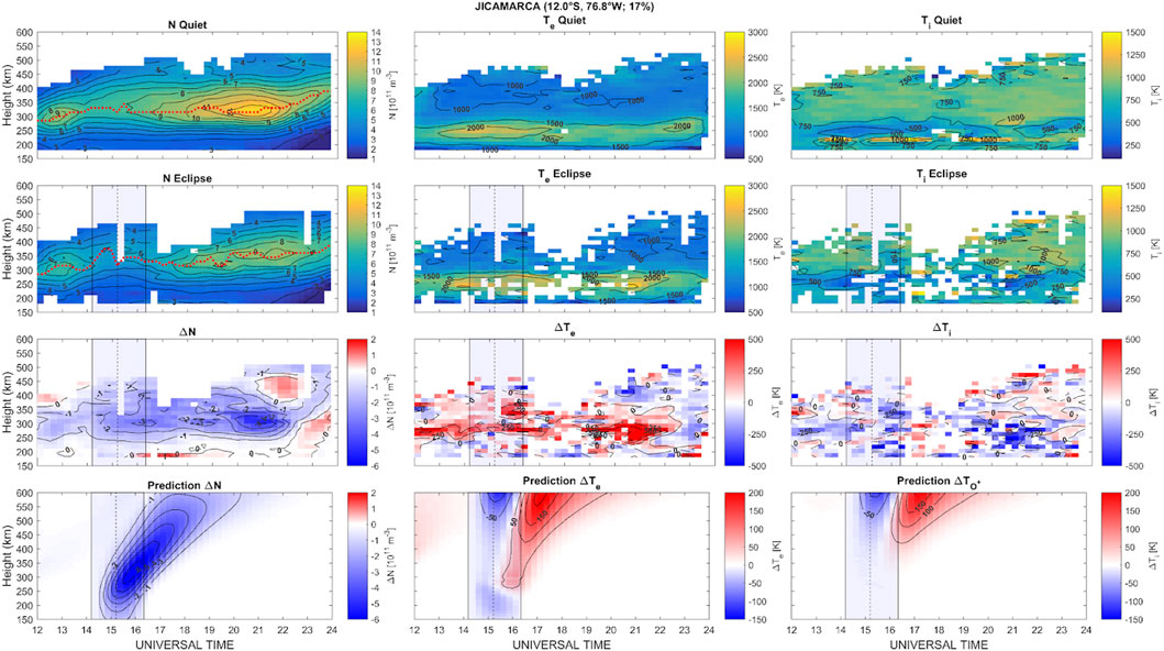
FIGURE 5. (first row)Vertical distribution of the reference days, (second row) eclipse day, and eclipse-modified differences of the (third row) measured and (fourth row) SUPIM-INPE modeled values of (first column) electron concentration (N), (second column) electron (Te), and (third column) ion (Ti) temperatures over time obtained by the Jicamarca Incoherent Scatter Radar (12.0°S, 76,8°W). Eclipse onset, maximum obscuration, and eclipse end (vertical lines) are calculated at 300 km height.

The electron density profile presents a reduction during most of the representation period (from 12 UT to 23 UT) at altitudes approximately between 200 and 400 km, indicating smaller density values during the eclipse day than the reference curve. Even so, during the eclipse obscuration, the largest decrease values are obtained after the maximum obscuration time at an altitude of around 300 km, agreeing with the predicted maximum decrease in height and time. Nevertheless, the magnitude of the maximum density decrease measured (∼3×10¹¹ m⁻³) is much lower than the predicted one (∼6×10¹¹ m⁻³), although its relative decrease percentage is much larger (40% and 12%, respectively). This disparity in the magnitude decrease is obtained because of the overall lower density obtained during the eclipse day relative to the quiet days (∼20% lower). On the other hand, the density decrease uplift predicted to occur after the eclipse obscuration cannot be observed due to the lack of information at high altitudes. Additionally, the density reduction values obtained after the start of the eclipse are maintained at low altitudes until ∼18 UT. Surprisingly, a much larger density decrease (∼40%) is observed at altitudes around 300 km, between approximately 20–22 UT. Moreover, an increase in density (∼10%) is obtained approximately 1 hour after the start of the previous decrease but at higher altitudes (between 400 and 500 km height). Neither this large density decrease nor the posterior increase at higher altitudes is reproduced by the model prediction.

The electron temperatures (Te) represented in Figure 5 show a large increase (∼250 K) located between 250 and 300 km height in most of the period (from 12 UT to 23 UT). This Te increase seems to be related to the overall differences found between the eclipse day and the reference pattern. This overall difference and a large number of data gaps hinder the correct interpretation of the eclipse’s impacts on the temperatures. Nevertheless, a clear Te increase of approximately 250 K is located at altitudes between 300 and 350 km height after the maximum obscuration time until the end of the eclipse traverse. During these same times, a Te increase was obtained by the model prediction at similar altitudes, although with a much smaller magnitude (about 50 K). The subsequent predicted uplift of the temperature increase is not observed due to the lack of information at high altitudes. Moreover, a much larger Te increase (∼500 K) is observed at altitudes between 200 and 250 km in height. This large temperature increase occurs simultaneously with the large density decrease found at 300 km in height (approximately between 19 UT and 22 UT).

Alternatively, the ion temperatures (Ti) show a much large variability. Even so, during the eclipse traverse, a clear Ti decrease of approximately 250 K is found around 300 km height, simultaneously with the increase of electron temperature previously indicated. Nevertheless, the prediction does not show ion temperature reductions at these altitudes during the eclipse. Indeed, the predicted reductions were expected at higher altitudes, but no ion temperature measurements are available at these heights. The lack of low altitude ion temperature reductions in the prediction is related to the fact that only atomic oxygen ion (O+) temperatures are represented, and those are the main species at altitudes above approximately 300 km height. Therefore, we assumed that the measured Ti decrease is mainly related to the response of molecular ion (NO+ and O2+) species during the eclipse. Unfortunately, no ion temperature information is available at altitudes higher than ∼450 km due to the filtering of data with high uncertainty. Therefore, a comparison of the predicted atomic oxygen temperature decrease and its posterior increase is not feasible. On the other hand, a Ti decrease is found between 200 and 250 km height which occurs simultaneously with the largest electron temperature increase that occurs after the eclipse (approximately between 19 UT and 22 UT).

3.5 Satellite Measurements

Figure 6A shows the in situ electron density (Ne) measurements made by the Swarm-A Lagmuir probes at 450 km altitude during the five selected geomagnetically quiet days and the eclipse day. The comparison of the latitudinal Ne profile of the day of the eclipse with the two closest trajectories to the eclipse both longitudinally and temporally (4th and 16th of December) are shown in Figure 6B. In the latitudinal profile at the beginning of the eclipse (from 15.1 UT to 15.8 UT), a slight decrease (−1.7×10⁵ e/cm³, −33%) is seen in the southern crest of the EIA during the day of the eclipse at meridian 70.6°W (close to Chillán meridian). Then, the percentage change of Ne close to the totality zone relative to the control days was consistent with the findings presented in (Cherniak and Zakharenkova, 2018; Valdes-Abreu et al., 2022). Furthermore, after the maximum of the eclipse (from 16.6 UT to 17.3 UT) a significant suppression of both EIA crests is seen (−6.1×10⁵ e/cm³, −75%), although already at the 94.0°W meridian over the Pacific Ocean. Although 117.4°W meridian exhibited an enhancement, a slight electron density decrease can still be observed between 3.5°S and 75°S (−2.4×10⁵ e/cm³, −48%) long after the end of the eclipse (from 18.2 UT to 18.9 UT). For purposes of determining the magnetic conjugate, it is important to note that the magnetic Equator is displaced from the geographic zero according to longitude (as seen in the black line of Figure 6A). As seen in the location of the EIA crests, the magnetic Equator location can be placed around −12° in longitude at the 17 UT in panel 6b.

FIGURE 6

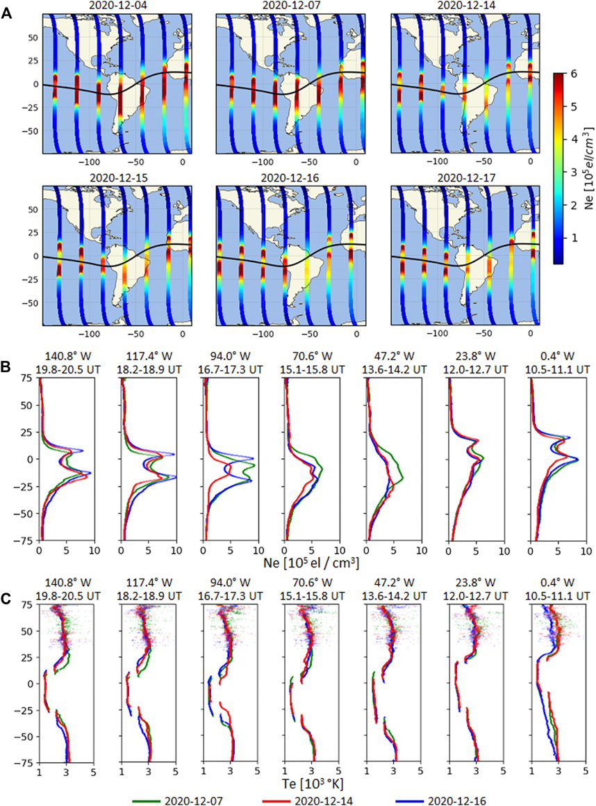
FIGURE 6. In situ plasma density (Ne) and electron temperatures (Te) measurements from the Swarm-A satellite at 450 km altitude. (A) Ne gathered through the satellite orbit is present over the map during the five selected geomagnetically quiet days and the eclipse day (2020–12–14) between 75°S and 75°N in the first 2 rows. Magnetic equator is indicated with a black line. (B) Comparison of the latitudinal Ne profile of the day of the eclipse (red line) with the two closest trajectories longitudinally and temporally (4th and 16th of December in green and blue, respectively). (C) Te data is presented in the same way as Ne data. The time interval of the satellites passes are indicated.

Additionally, Te obtained by the Swarm-A Lagmuir probes are shown in Figure 6C. The comparison of the measurements obtained during eclipse day and the closest trajectories shows a temperature response to the eclipse inverse to the response of the electron density. A temperature increase is found in the latitudinal profiles at the meridians 70.6°W, 94°W, and 114°W. Moreover, this increase is simultaneous to the Ne reductions previously indicated, showing the largest differences at the suppressions of the EIA crests. At the beginning of the eclipse (from 15.1 UT to 15.8 UT), Te shows its maximum increases near the crests of the EIA at 0.4°S (812 K, 54%) and 30.7°S (656 K, 41%). After the eclipse totality (from 16.6 UT to 17.3 UT), increases are found at both hemispheres, but a much larger Te increase is observed in the Southern hemisphere at 27.3°S (1243 K, 79%). Again, it is relevant to highlight that panel 6c is represented in geographic latitudes. Finally, long after the end of the eclipse (from 18.2 UT to 18.9 UT), large remaining increases are found at 22.7°S (735 K, 49%). It is relevant to note that the Te differences obtained by Swarm-A in the comparisons of the other transects are around 10%. These temperature observations are different to the prediction both in magnitude and location (see supplementary material of Martínez-Ledesma et al., 2020). The model prediction provided initial temperature decreases of up to 400 K at the eclipse totality that were not captured by the satellite. Moreover, after the eclipse obscuration, the model expected maximum temperature increases of 300 K near the eclipse totality (at ∼38°S) but about four times larger increases are observed at lower latitudes (of ∼1250 K at 27.3°S). Nevertheless, the model correctly reproduces the overall conjugate response to the eclipse, increasing the temperatures of both hemispheres after the solar obscuration.

3.6 Model-measurement statistical comparison

Different metrics are presented in Tables 1, 2 for evaluating the performance of the model predictions when compared to the measured data. The comparisons for the daily variation (12 UT to 24 UT) are shown in Table 1. Alternatively, Table 2 presents the comparison results during the eclipse obscuration time. The number of data pairs evaluated in each case (Num) is also listed in both Tables. The results obtained suggest that the model was able to reproduce with high accuracy both the daily variation and the eclipse impacts at low heights (layers E and F1) in the majority of the stations evaluated. This can be seen in the low NRMSE found between the measured and predicted values of foE at Tucumán, Chillán, and Bahia Blanca stations and their very high correlation values. It is worth mentioning that the high correlation values obtained at Bahía Blanca during the eclipse event are distorted due the lack of measurements in lower regions and provide non-significant results. Non-etheless, the comparison of foE at Jicamarca station provides NRMSE of approximately 11% and much lower correlation coefficients (r = 0.65 and ρ = 0.73) during the eclipse time. The Jicamarca station differences are related to obtaining foE values lower than the prediction in all the observation period and to the high variability of the values measured (see Figure 2). Similar results are observed for the F1 layer, in which high correlations are obtained in all stations except in the daily variation of Jicamarca station. Even so, higher NRMSE are found in all the evaluated stations due to the usage of an iso-height curve at 190 km for the determination of the prediction of this layer.

TABLE 1

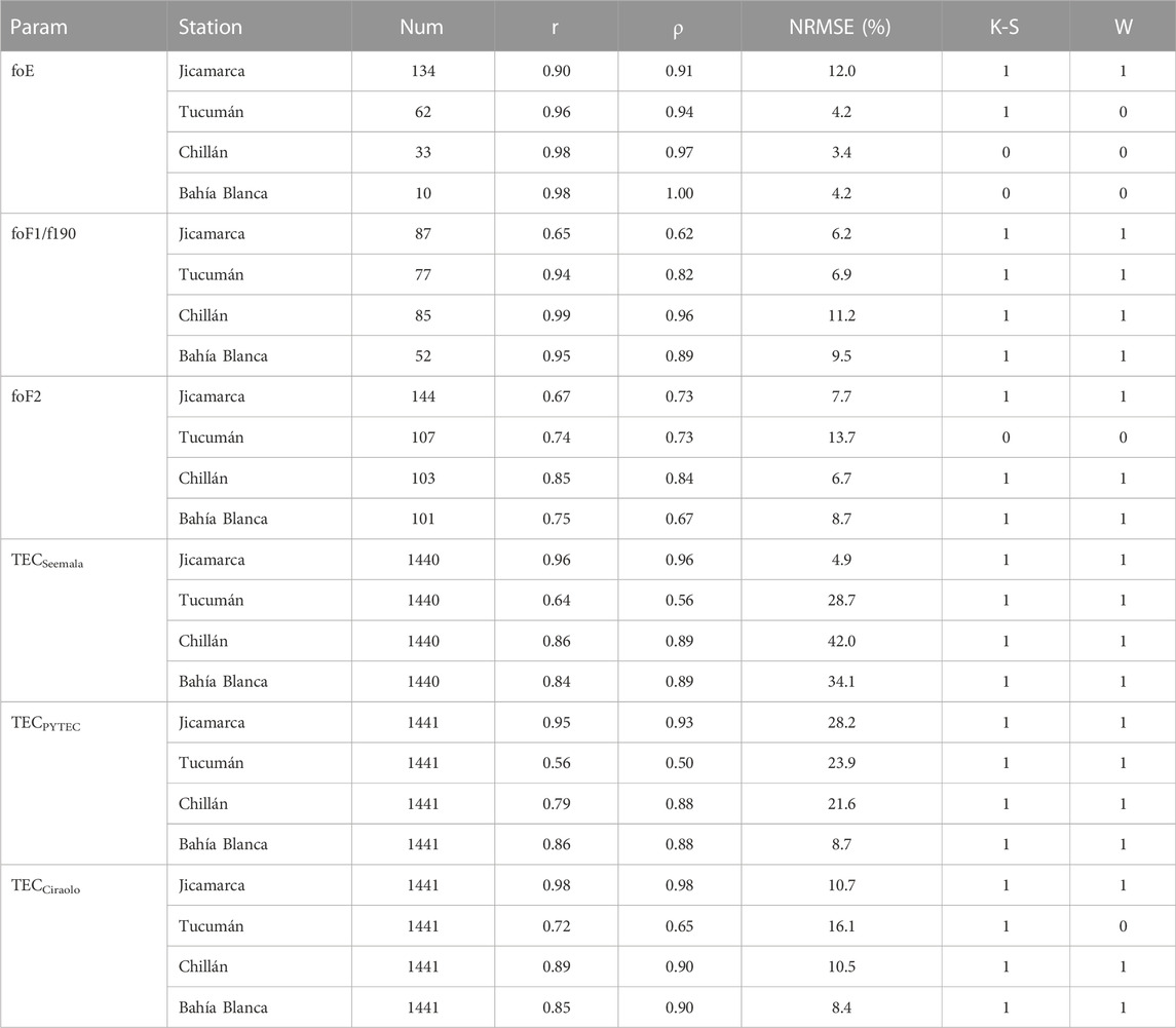
TABLE 1. Model-Measurement statistical comparison for window interval (12–24 UT).

TABLE 2

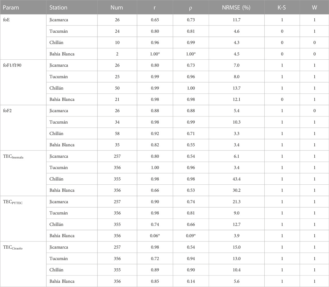
TABLE 2. Model-measurement statistical comparison for eclipse time interval (*non-significant values).

At the F2 layer, the comparison indicates small NRMSE (<10.3%) at all stations during the eclipse periods. Even so, during this period, a worst model reproducibility is obtained at Bahia Blanca station highlighted by the low correlation coefficient values (r = 0.75 and ρ = 0.67). This could be related to the faint foF2 modification observed at Bahia Blanca during the eclipse obscuration. Moreover, the large difference observed between the Pearson and Spearman coefficients at Chillán station during the eclipse (r = 0.92 and ρ = 0.71) are related to a larger decrease of foF2 during the maximum obscuration time (Figure 2), which presents a clear non-linear response to the solar radiation reduction. On the other hand, the overall daily variation shows a worst reproducibility of the model prediction. In this case, there are lower correlation values and higher NRMSE (up to 13.7%), that are mainly related to the incapacity to reproduce the variations observed after the eclipse obscuration in Tucumán, Chillán, and Bahia Blanca stations (starting approximately at 20 UT). It is relevant to highlight that Tucumán shows the largest NRMSE value in both evaluation periods due to a large foF2 increase that starts during the eclipse recovery phase at ∼17 UT.

The statistical comparison between modeled and calibrated TEC shows that none of the selected calibration methods follow SUPIM-INPE prediction consistently at all stations. The Seemala method (Seemala and Valladares, 2011) provides very large NRMSE (up to ∼43%) at Chillán and Bahía Blanca stations during both evaluated periods. This effect is related to an overall TEC decrease of this method with the increasing latitude (see Supplementary Material, Supplementary Figure S1). Alternatively, the Ciraolo method (Ciraolo et al., 2007) shows the smallest NRMSE (<16.1%) but provides small values of correlation both at Jicamarca and Bahía Blanca during the eclipse (ρ = 0.54 and −0.14, respectively). These stations show large differences of Pearson and Spearman correlations, demonstrating the non-linear relationship and the large variability of the measured results. Finally, the PYTEC method obtained similar difference values in all stations during the eclipse except at Jicamarca. At this station, the NRMSE obtained is 21.3% but the Spearman correlation is higher than in the other two methods (ρ = 0.74), suggesting that somehow the measurements better reproduce the eclipse impact prediction with this method. It should be highlighted that the smallest NRMSE during the eclipse are found with this method at Bahía Blanca station (3.9%), but no correlation is obtained with the prediction (ρ = −0.09, although with no statistical significance). On the other hand, the comparison of the different TEC methods during the 12 h period provides similar differences and high correlations at all stations except at Tucumán station. Indeed, Tucuman presented a clear reduction of the TEC after the eclipse (∼18 UT) obtained with the three methods which were not predicted.

Additionally, Tables 1, 2 present the test result (h) of the two non-parametric hypothesis tests evaluated. In our study, a test result h = 0 implies accepting the null hypothesis with a significance level of 0.05, and alternatively h = 1 means rejecting it. Therefore, the rejection of the null hypothesis of the K-S test indicates that the modeled and measured data series are from different distributions. Similarly, the rejection of the null hypothesis of the W test implies that they have different median distribution values.

The K-S statistical test produced very few acceptations of the hypothesis because the empirical and modelled data have different statistical distributions (due to the random nature of the multiple input variations that may impact the measurements). This is particularly true for the different TEC calibrations, in which none of the tests the null hypothesis was accepted either for the daily variation or the eclipse time. In these cases, the W-test only accepted the null hypothesis on the Ciraolo calibration at Tucumán in the daily variation. These results indicate that the model predicted statistical distributions are different from the distributions of the measured values in all the TEC methods evaluated, but also the medians of the distributions are not identical. This highlights the difficulties to properly model the TEC and suggests further studies in this area to accurately reproduce the ionospheric response.

On the other hand, the K-S test accepted the null hypothesis for the foE in the majority of cases (i.e., at Chillán and Bahía Blanca during the daily variation and at Tucumán, Chillán, and Bahía Blanca during the eclipse). Also, in these cases the W-test for the foE indicated that the medians were identical. These results highlight the high accuracy of the model to properly reproduce the measurements at all locations but Jicamarca. Alternatively, the K-S and W tests did not accepted the null hypothesis in almost all study cases for foF1 and foF2. This may be related to the differences in the selected height to predict the foF1 (i.e., at 190 km by Martínez-Ledesma et al., 2020) and the variability of responses of the foF2 indicated in the literature (e.g., Le et al., 2009).

4 Discussion

Historically, the SUPIM model has been used to reproduce the South American ionosphere with high accuracy (e.g., Bailey et al., 1993; Paula et al., 1996; Souza et al., 2000a; 2000b). The adaptations that have been made to this model at INPE have improved its capability to reproduce the local characteristics and disturbance conditions over the equatorial and low latitudes ionosphere on the Peruvian and Brazilian longitudes (e.g., Batista et al., 2006, 2011; Souza et al., 2010, 2013; Abdu et al., 2013; Nogueira et al., 2013; Santos et al., 2016, 2017; Bravo et al., 2017, 2019). Although the SUPIM model was previously used to study eclipse conditions (MacPherson et al., 2000), the SUPIM-INPE version was further modified to evaluate the 2 July 2019, total solar eclipse (Bravo et al., 2020). These later modifications allowed its usage to predict the following eclipse: the 14 December 2020, total solar eclipse (Martínez-Ledesma et al., 2020).

One of the main characteristics of the total eclipse event of 14 December 2020, is that its totality occurred shortly before noon (10-11 SAT), allowing to clearly see the response of the E and F1 layers, in opposition to the 2 July 2019 total solar eclipse, in which the totality occurred in the evening hours (16-17 SAT) when the E and F1 layers begin to disappear. In these layers, the model predictions are very close to the measured responses for almost all selected ionospheric stations, both during the eclipse obscuration and the rest of the time period (see Figure 2). On the other hand, the same cannot be said for foF2 and TEC, where the predictions are not so close during the eclipse for Tucumán. Additionally, the variations of these parameters after the eclipse in Tucumán, Chillán, and Bahía Blanca are not reproduced by the prediction, suggesting that there could be late effects of the eclipse, which are not being considered by the model. These results are also verified by the empirical and modeled data differences and their correlation coefficients (Tables 1, 2).

Multiple effects impacted the ionosphere during the 2 July 2019 eclipse, which occurred in a similar region of the low latitude Southamerican sector. There was an anticipated pre-reversal enhancement effect deduced from observations (Bravo et al., 2020), and confirmed later by Jonah et al. (2020), that altered the equatorial electrodynamics. Jonah et al. (2020) suggests that it was the result of a perturbed ionospheric dynamo due to the eclipse. In addition, the SUPIM-INPE model used for the evaluation of the eclipse by Bravo et al. (2020) did not considered the interaction with atmospheric gravity waves due to this eclipse observed by Maurya et al. (2020) and Vargas et al. (2022), and the generation of TIDs observed by Eisenbeis & Occhipinti (2021). Neither does the model consider the changes in the neutral composition, specifically in the O/N2 rate, recently observed by Aryal et al. (2020a) from GOLD mission data during this event.

It is important to note that there are evidence of equatorial counter electrojets (CEJs) frequently seen by magnetometers during the December solstices (Mayaud, 1977). These equatorial CEJs are even pronounced during Sun, Moon, Earth alignment days, i.e., full moon, new moon and therefore during the occurrence of eclipses (Bhaskar et al., 2011; St-Maurice et al., 2011; Panda et al., 2015). These conditions are met during the 14 December 2020, total solar eclipse. The main impact of the CEJ would be poor feeding of EIA due to the severely weakened fountain effect on the eclipse day and adjacent days. However, this effect has not been considered in the choice of quiet days to make the reference curve. The selected dates of December 04 and 07 are further from the eclipse date than days 15, 16 and 17. This could slightly affect the results for equator and low latitudes in de Haro Barbas et al. (2022), and particularly, in the results shown in Figures 3, 4 of this work. But it would not affect Figures 5, 6, since this comparison analysis considers other days.

Additionally, when we observe the evolution of the TEC along the magnetic meridian (Figure 3), the shape of the ΔTEC decrease obtained is very similar to that predicted by the model, although twice as large. This difference is mainly observed in the crests of the EIA on both sides of the magnetic equator. This phenomenon can be corroborated with the in situ measurements provided by the Swarm-A (Figure 6). To provide a further verification, Figure 7 shows that the same decrease in electron density can be seen in the South crest of the EIA at longitudes of the Brazilian sector several hours after the eclipse traverse. These data were obtained from the Ionogram-Derived Characteristics of DIDBase (https://giro.uml.edu/didbase/scaled.php). Although Cachoeira Paulista (22.7°S, 45°W) had a maximum of 30% of eclipse obscuration, no differences in foF2 were observed during the eclipse obscuration, as previously indicated by Resende et al. (2022). However, a reduction can be observed after the time of the eclipse, at approximately 19 UT. This foF2 reduction is very similar to what was observed in Tucumán station in Figure 2, both of which were not correctly represented in the prediction. It is relevant to note that both Cachoeira Paulista and Tucumán have similar magnetic latitudes (∼-20°). Indeed, the largest density reduction observed in foF2 at Tucumán and Cachoeira Paulista occurs simultaneously to a foF2 increase in Chillán and Bahía Blanca (located at a magnetic latitude of ∼ -26° and ∼-30°, respectively), at approximately 20 UT (Figure 2). Simultaneously, a density enhancement is also observed in the northern hemisphere in the TEC of Figure 3 and a decrease of electron density measured by the Jicamarca ISR at 300 km (Figure 5). The equatorial density decrease is also associated with an increase of the electron temperature and a posterior density increase at higher altitudes (400 km height). These results suggest a possible modification of the fountain effect that is also supported by a small increase of the vertical drifts measured by the ISR (not shown) that commonly occurs during the evening. Nevertheless, there is no clear indication of the origin of the interhemispheric TEC asymmetry observed.

FIGURE 7

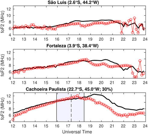
FIGURE 7. foF2 variations over three stations in the Brazilian sector for the day of the eclipse (14 December 2020). The measured data is represented in red circles and the reference curve in black. Eclipse onset, maximum obscuration, and eclipse end (vertical lines) is calculated at 300 km height.

Since the photoelectrons have a key role in keeping the electrons warmer than the ions, a reduction in the temperature of the electrons is expected during the eclipse. Nevertheless, early ISR measurements at Jicamarca (on the eclipse of 11 September 1969) obtained temperature increases around 400–500 km (Sterling et al., 1972). Alternatively, measurements of the Millstone Hill ISR at mid latitudes have observed electron temperature decreases up to 700 K in the F region during eclipses (e.g., Salah et al., 1986). The SUPIM-INPE prediction indicated a small decrease followed by a large temperature increase that would grow with altitude. Temperature decreases and posterior smaller enhancements have been previously observed at the Millstone Hill ISR after the maximum obscuration time by Goncharenko et al. (2018). Nevertheless, in our study, the observations obtained by the Jicamarca ISR indicate only an increase of approximately 250 K around 350 km height after the maximum eclipse obscuration (see Figure 5). To the best of the authors’ knowledge, there is no clear explanation of the disparity of eclipse impacts on electron temperatures. Additionally, Figure 6 shows a clear temperature enhancement measured by Swarm-A at the low latitude region after the maximum of the eclipse (from 16.6 UT to 17.3 UT). This temperature increase is found at both hemispheres and it is coincident with the locations at which the EIA crests present an electron density reduction. This electron temperature enhancement at 450 km height agrees with the predicted uplift of the temperature increase after the eclipse obscuration shown in Figure 5, providing additional temperature information that was not observed by the Jicamarca ISR at such altitudes. Both the electron temperature changes observed in ISR and Swarm-A are underestimated by the prediction. The same was observed in Aryal et al. (2020b), where the TIEGCM model grossly underestimated the eclipse-induced temperature change observed in the GOLD mission near totality of the 2 July 2019 total solar eclipse by more than 150 K. On the other hand, for the annular solar eclipse of 21 June 2020, Huang et al. (2020) using measurements from the Swarm-B and C satellites found no visible effects of the temperatures.

The results of the statistical comparison indicate that the study of Martínez-Ledesma et al. (2020) provided an accurate overall prediction of the ionospheric impact of the eclipse, although large differences are obtained at high altitudes (i.e., foF2 and TEC) after the eclipse event. These differences are related to the difficulty to reproduce the plasma dynamics at high altitudes in the equatorial and mid latitude region. Indeed, there may be two input factors that are not considered in the model that could make the simulations predicted by SUPIM-INPE not agree with the observations after the eclipse. One input factor is the thermospheric neutral wind that modifies the eclipse-induced TEC reduction and affects the neutral temperature and mass density responses through advection (Dang et al., 2018; Cnossen et al., 2019). The other factor could be the changes in the O/N2 ratio due to the eclipse that should be very important in mid-latitudes.

The O/N2 ratio can be directly obtained from Global UltraViolet Imager, TIMED/GUVI, observations (http://guvitimed.jhuapl.edu/). However, near the geographic zones of the maximum of the eclipse, GUVI generates a gap zone, due to the South Atlantic Anomaly (figure not shown). To avoid this constraint, we analyzed data from the Global-scale Observations of the Limb and Disk (GOLD) mission over South America (https://gold.cs.ucf.edu/). We analyzed the L2 product ON2 (or O/N2 column density ratio) derived from daytime disk scan measurements. This is an integrated daily product for approximately 68 disk scan measurements performed per day by GOLD in a nominal operation.

Figure 8 shows the daily O/N2 for the 13, 14, and 15th of December 2020. Additionally, Jicamarca, Tucumán, Chillán, and Bahía Blanca locations are marked as cyan dots for visual reference. In this figure, it can be observed that during the eclipse day the O/N2 ratio is considerably enhanced with respect to the previous and next days, in particular at Bahia Blanca station. During the 13th and 15th of December, the O/N2 (around the marked stations) varies approximately between 0.6 and 0.7, while during the eclipse day on the 14th it can be observed that such ratio is varying between 0.7 and 0.85, approximately. It should be mentioned that, in this case, the O/N2 is a daily integrated product (about 68 scans) which means that the observed enhancement, during the eclipse day, is significant. These changes are equivalent to an increase of ∼30% under eclipse conditions, which is considerably less than the ∼80% obtained by Aryal et al. (2020a) from GOLD measurements for the 2 July 2019 total solar eclipse. Thus, the variations in the O/N2 ratio is an input that the model should incorporate in the future, specially at mid-latitude stations.

FIGURE 8

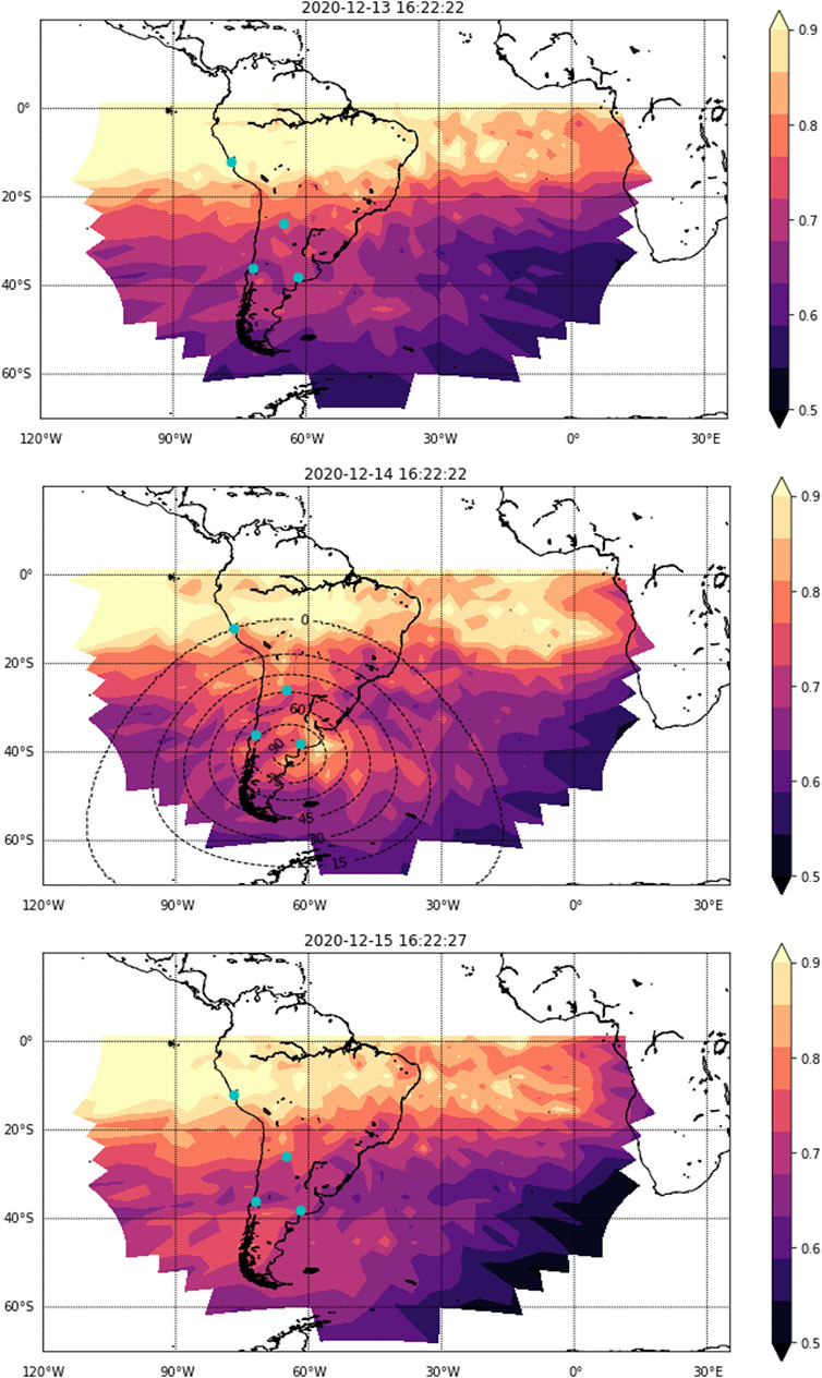
FIGURE 8. O/N2 ratio (L2 data product) from GOLD daytime disk scan measurements (https://gold.cs.ucf.edu/). The cyan circles show the locations of the ionospheric stations used in this work.

5 Conclusion

In this work we conducted a detailed evaluation of the SUPIM-INPE model under eclipse conditions using multi-instrument data and GNSS derived TEC. In particular, we studied the different ionospheric impacts of the 14 December 2020 eclipse at different South American stations covering different latitudes and eclipse obscuration percentages.

The comparison results suggest that the SUPIM-INPE model estimates accurately the effects produced by the solar eclipse. At the different layers (i.e., E, F1, and F2 layers), the model does not present variations during the eclipse greater than ∼14% in relation to the measured values. Moreover, the model predicts the conditions for the E layer very well, except for a slightly larger difference at the Jicamarca station. For the F1 layer, there are very good agreements for the Jicamarca and Tucumán stations, while for the higher latitude stations, Chillán and Bahía Blanca, an increase in the difference is observed. In the case of the F2 layer, an excellent agreement is observed in all the stations, with differences that do not exceed 8%.

Additionally, three different methods of obtaining TEC are used to compare with the model prediction. Although these methods provide TEC with different amplitudes, all of them obtain similar reductions to the prediction, except at Bahía Blanca station and during the hours after the eclipse. In particular, the Tucumán station shows a significant decrease after 19 UT, while Chilllán and Bahía Blanca show a peak centered at 22 UT (also seen in foF2), all effects that cannot be reproduced in the model. This suggests the occurrence of later effects of the eclipse (and seen in the literature). A similar situation is observed in the temporal evolution of the TEC along the magnetic meridians. The general trend of the TEC decrease is similar to the predicted profile although there exist differences in amplitude. Additionally, the TEC shows effects on the northern crest of the EIA similar to those predicted.

A statistical comparison has been performed by determination of the percentual differences and correlation coefficients of the measured and predicted data both for the eclipse period and for the overall daily variation. Results show that for most ionospheric parameters there is a similar tendency with the predicted curves, whether this is linear or non-linear. On the other hand, the NRMSE values obtained were often less than 10%, which, together with high correlation coefficients, suggest a good performance in terms of modelling. These differences are much greater when it comes to TEC (as expected, due to the different calibration techniques). Again, quantitatively it is observed that the prediction for Bahía Blanca does not provide an accurate response at high altitudes.

Additionally, it has been shown that both the electron temperature changes, as observed by the Jicamarca ISR and the in situ measurements of the Swarm-A satellite, are underestimated by the prediction.

Future versions of the SUPIM-INPE for eclipse conditions should consider additional effects not yet considered within the model. In particular, it is required to include the variations of the thermospheric winds and changes in composition, specifically in the O/N2 ratio, as observed from GOLD satellite measurements. Nevertheless, the SUPIM-INPE model has proven to be a suitable model to understand and predict ionospheric variability under eclipse conditions.

Data availability statement

The original contributions presented in the study are included in the article/Supplementary Material, further inquiries can be directed to the corresponding author.

Author contributions

MB, MM-L, JS, BU, and AF contributed to conception and design of the study. MB, JS, and MM-L adapted the model. MM, EO, EG, ER, LP, EC, RL, MM, PM, MS, and MC commissioned the measurement campaign. BU, CV, MM, and JN curated the ionosonde data. MM, JN, SB, JV-A, CR, and JV worked with the satellite data. BH, AE, and BU performed the statistical analysis. MB, MM, MM-L, BH, BU, AE, and JV participated in the discussion of the article. All authors contributed in wrote the first draft of the manuscript, to manuscript revision, read, and approved the submitted version.

Acknowledgments

In this study, data from the Jicamarca Radio Observatory (JRO) Incoherent Scatter Radar has been used. The JRO is a research facility of the Instituto Geofísico del Perú operated with support from the National Science Foundation through Cornell University under award AGS-1732209. Access to the GNSS data was kindly provided by the International GNSS Service (IGS, www.igs.org), by the Centro Sismológico Nacional (CSN) of the Universidad de Chile (www.sismologia.cl), by the Red Argentina de Monitoreo Satelital Continuo (RAMSAC) of the Instituto Geográfico Nacional de la República Argentina (www.ign.gob.ar), by the Rede Brasileira de Monitoramento Contínuo dos Sistemas GNSS (RBMC) of the Instituto Brasileiro de Geografia e Estatística (ww2.ibge.gov.br), the Red Geodésica Nacional Activa (REGNA) of the Instituto Geográfico Militar del Uruguay (ftp://pp.igm.gub.uy) and from Colombian network (MAGNA, https://geoportal.igac.gov.co). Cesar Valladares kindly provided access to the Low-Latitude Ionospheric Sensor Network (LISN, http://lisn.igp.gob.pe/). LISN is a project led by the University of Texas at Dallas in collaboration with the Geophysical Institute of Perú. We acknowledge Tucumán Space Weather Center (TSWC), Argentina, https://spaceweather.facet.unt.edu.ar/for providing the AIS-INGV data. We thank the European Space Agency that supports the Swarm mission and acknowledge the engineers and research team of the GOLD mission (https://gold.cs.ucf.edu/). MB acknowledges CONICYT/FONDECYT Postdoctorado 3180742, and together with MS to FONDECYT REGULAR 1211144. MM-L acknowledges the support of ANID/FONDECYT Postdoctorado 3220581 and Comité Mixto ESO-Chile ORP061/19. JV-A acknowledges the support of ANID/Scholarship Program/Doctorado Nacional/2018-21181599. BF, BH, and AG, AE acknowledge Project PIP 2957 (CONICET). JV and SB acknowledge the support of ANID/FONDECYT 1190703 and the US AFOSR PI FA9550-20-1-0189. MM acknowledges project PIUNT 26/E-689. MM, BF, BH, AG, and AE acknowledge project PICT 2018-04447 projects. The authors thank MSc. Eduardo Gutiérrez for his guidance on statistics.

Conflict of interest

The authors declare that the research was conducted in the absence of any commercial or financial relationships that could be construed as a potential conflict of interest.

The handling editor PK is currently organizing a Research Topic with the author VJA.

Publisher’s note

All claims expressed in this article are solely those of the authors and do not necessarily represent those of their affiliated organizations, or those of the publisher, the editors and the reviewers. Any product that may be evaluated in this article, or claim that may be made by its manufacturer, is not guaranteed or endorsed by the publisher.

Supplementary material

The Supplementary Material for this article can be found online at: https://www.frontiersin.org/articles/10.3389/fspas.2022.1021910/full#supplementary-material

References

Abdu, M. A., Souza, J. R., Batista, I. S., Fejer, B. G., and Sobral, J. H. A. (2013). SporadicElayer development and disruption at low latitudes by prompt penetration electric fields during magnetic storms. J. Geophys. Res. Space Phys. 118, 2639–2647. doi:10.1002/jgra.50271

CrossRef Full Text | Google Scholar

Adekoya, B. J., and Chukwuma, V. U. (2016). Ionospheric F2 layer responses to total solar eclipses at low and mid-latitude. J. Atmos. Sol. Terr. Phys. 138, 136–160. doi:10.1016/j.jastp.2016.01.006

CrossRef Full Text | Google Scholar

Araujo-Pradere, E. A., and Fuller-Rowell, T. J. (2002). Storm: An empirical storm-time ionospheric correction model, 2, Validation. Radio Sci. 37 (5), 4-1–4-14. doi:10.1029/2002RS002620

CrossRef Full Text | Google Scholar

Arikan, F., Nayir, H., Sezen, U., and Arikan, O. (2008). Estimation of single station interfrequency receiver bias using GPS-TEC. Radio Sci. 43, RS4004. doi:10.1029/2007RS003785

CrossRef Full Text | Google Scholar

Aryal, S., Evans, J. S., Correira, J., Burns, A. G., Wang, W., Solomon, S. C., et al. (2020a). First global-scale synoptic imaging of solar eclipse effects in the thermosphere. J. Geophys. Res. Space Phys. 125, \. doi:10.1029/2020JA027789

CrossRef Full Text | Google Scholar

Aryal, S., Evans, J. S., Solomon, S. C., Burns, A. G., Correira, J., Dang, T., et al. (2020b2020). Global-scale data-model comparison of the July 2nd, 2019 total solar eclipse’s thermospheric effect. EGU General Assem., EGU2020–13197. Online, 4–8 May 2020. doi:10.5194/egusphere-egu2020-13197

CrossRef Full Text | Google Scholar

Bailey, G. J., and Balan, N. (1996). “A low-latitude ionosphere-plasmasphere model,” in Solar-terrestrial energy program: Handbook of ionospheric models Center for Atmospheric and space Sciences, 173–206. Editor R. W. Schunk (Logan, Utah: Utah State University).

Google Scholar

Bailey, G. J., Balan, N., and Su, Y. Z. (1997). The Sheffield University plasmasphere ionosphere model - a review. J. Atmos. Sol. Terr. Phys. 59 (13), 1541–1552. doi:10.1016/S1364-6826(96)00155-1

CrossRef Full Text | Google Scholar

Bailey, G. J., and Sellek, R. (1990). A mathematical model of the Earth's plasmasphere and its application in a study of He at L = 3. Ann. Geophys. 8 (3), 171–189.

Google Scholar

Bailey, G. J., Sellek, R., and Rippeth, Y. (1993). A modelling study of the equatorial topside ionosphere. Ann. Geophys. 11 (4), 263–272.

Google Scholar

Batista, I. S., Abdu, M. A., Souza, J. R., Bertoni, F., Matsuoka, M. T., Camargo, P. O., et al. (2006). Unusual early morning development of the equatorial anomaly in the Brazilian sector during the Halloween magnetic storm. J. Geophys. Res. 111, A05307. doi:10.1029/2005JA011428

CrossRef Full Text | Google Scholar

Batista, I. S., Diogo, E. M., Souza, J. R., Abdu, M. A., and Bailey, G. J. (2011). “Equatorial ionization anomaly: The role of thermospheric winds and the effects of the geomagnetic field secular variation,”. Editors M. A. Abdu, D. Pancheva, and A. Bhattacharyya (London: Springer), 2, 317–328. doi:10.1007/978-94-007-0326-1_23Aeronomy Earth's Atmos. Ionos.

CrossRef Full Text | Google Scholar

Beynon, W. J. G. (1955). Solar eclipses and the ionosphere. Nature 176 (4490), 947–948. doi:10.1038/176947a0

CrossRef Full Text | Google Scholar

Bhaskar, A., Purohit, A., Hemalatha, M., Pai, C., Raghav, A., Gurada, C., et al. (2011). A study of secondary cosmic ray flux variation during the annular eclipse of 15 January2010 at rameswaram, India. Astropart. Phys. 35, 223–229. doi:10.1016/j.astropartphys.2011.08.003

CrossRef Full Text | Google Scholar

Bowles, K. L., Ochs, G. R., and Green, J. L. (1962). On the absolute intensity of incoherent scatter echoes from the ionosphere. J. Res. NBS D. 66, 395–407. doi:10.6028/jres.066d.041

CrossRef Full Text | Google Scholar

Bravo, M. A., Batista, I. S., Souza, J. R., and Foppiano, A. J. (2017). Equatorial ionospheric response to different estimated disturbed electric fields as investigated using Sheffield University Plasmasphere Ionosphere Model at INPE. J. Geophys. Res. Space Phys. 122 (10), 527. 511–10. doi:10.1002/2017JA024265

CrossRef Full Text | Google Scholar

Bravo, M. A., Batista, I. S., Souza, J. R., and Foppiano, A. J. (2019). Ionospheric response to disturbed winds during the 29 October 2003 geomagnetic storm in the Brazilian sector. J. Geophys. Res. Space Phys. 124, 9405–9419. doi:10.1029/2019JA027187

CrossRef Full Text | Google Scholar

Bravo, M., Martínez-Ledesma, M., Foppiano, A., Urra, B., Ovalle, E., Villalobos, C., et al. (2020). First report of an eclipse from Chilean ionosonde observations: Comparison with total electron content estimations and the modeled maximum electron concentration and its height. J. Geophys. Res. Space Phys. 125, e2020JA027923. doi:10.1029/2020JA027923

CrossRef Full Text | Google Scholar

Cheng, K. H., Huang, Y. N., and Chen, S. W. (1992). Ionospheric effects of the solar eclipse of September 23, 1987, around the equatorial anomaly crest region. J. Geophys. Res. 97 (A1), 103–111. doi:10.1029/91JA02409

CrossRef Full Text | Google Scholar

Cherniak, I., and Zakharenkova, I. (2018). Ionospheric total electron content response to the great American solar eclipse of 21 August 2017. Geophys. Res. Lett. 45 (3), 1199–1208. doi:10.1002/2017gl075989

CrossRef Full Text | Google Scholar

Chukwuma, V., and Adekoya, B. (2016). The effects of March 20 2015 solar eclipse on the F2 layer in the mid-latitude. Adv. Space Res. 58 (9), 1720–1731. doi:10.1016/j.asr.2016.06.038

CrossRef Full Text | Google Scholar

Ciraolo, L., Azpilicueta, F., Brunini, C., Meza, A., and Radicella, S. M. (2007). Calibration errors on experimental slant total electron content (TEC) determined with GPS. J. Geod. 81, 111–120. doi:10.1007/s00190-006-0093-1

CrossRef Full Text | Google Scholar

Cnossen, I., Ridley, A. J., Goncharenko, L. P., and Harding, B. J. (2019). The response of the ionosphere-thermosphere system to the 21 August 2017 solar eclipse. JGR. Space Phys. 124, 7341–7355. doi:10.1029/2018JA026402

CrossRef Full Text | Google Scholar

Dang, T., Lei, J., Wang, W., Zhang, B., Burns, A., Le, H., et al. (2018). Global responses of the coupled thermosphere and ionosphere system to the August 2017 Great American Solar Eclipse. J. Geophys. Res. Space Phys. 123, 7040–7050. doi:10.1029/2018JA025566

CrossRef Full Text | Google Scholar

de Haro Barbás, B. F., Bravo, M., Elías, A. G., Martínez-Ledesma, M., Molina, G., Urra, B., et al. (2022). Longitudinal variations of ionospheric parameters near totality during the eclipse of December 14, 2020. Adv. Space Res. 69 (5), 2158–2167. doi:10.1016/j.asr.2021.12.026

CrossRef Full Text | Google Scholar

Dow, J. M., Neilan, R. E., and Rizos, C. (2009). The international GNSS service in a changing landscape of global navigation satellite systems. J. Geod. 83 (3), 689–198. doi:10.1007/s00190-009-0315-4

CrossRef Full Text | Google Scholar

Eisenbeis, J., and Occhipinti, G. (2021). TEC depletion generated by the total solar eclipse of 2 July 2019. JGR. Space Phys. 126, e2021JA029186. doi:10.1029/2021JA029186

CrossRef Full Text | Google Scholar

Evans, J. V. (1969). Theory and practice of ionosphere study by thomson scatter radar. Proc. IEEE 57, 496–530. doi:10.1109/PROC.1969.7005

CrossRef Full Text | Google Scholar

Fejer, B. G., Jensen, J. W., and Su, S.-Y. (2008). Quiet time equatorial F region vertical plasma drift model derived from ROCSAT-1 observations. J. Geophys. Res. 113, A05304. doi:10.1029/2007JA012801

CrossRef Full Text | Google Scholar

Forecast Centre (ASFC). Forecast centre (ASFC). Hist. Geophys. Space Sci. 9 (1), 53–63.

Google Scholar

Friis-Christensen, E., Lühr, H., Knudsen, D., and Haagmans, R. (2008). Swarm-An Earth observation mission investigating geospace. Adv. Space Res. 41 (1), 210–216. doi:10.1016/j.asr.2006.10.008

CrossRef Full Text | Google Scholar

Gibbons, J. D., and Chakraborti, S. (2011). Nonparametric statistical inference. 5th Ed. Boca Raton, FL: Chapman & Hall/CRC Press, Taylor & Francis Group. 9781439896129.

Google Scholar

Gómez, D. D. (2021). Ionospheric response to the December 14, 2020 total solar eclipse in South America. JGR. Space Phys. 126, e2021JA029537. doi:10.1029/2021JA029537

CrossRef Full Text | Google Scholar

Goncharenko, L. P., Erickson, P. J., Zhang, S. R., Galkin, I., Coster, A. J., and Jonah, O. F. (2018). Ionospheric response to the solar eclipse of 21 August 2017 in Millstone Hill (42N) observations. Geophys. Res. Lett. 45, 4601–4609. doi:10.1029/2018GL077334

CrossRef Full Text | Google Scholar

Hedin, A. E., Fleming, E. L., Manson, A. H., Schmidlin, F. J., Avery, S. K., Clark, R. R., et al. (1996). Empirical wind model for the upper, middle and lower atmosphere. J. Atmos. Terr. Phys. 58 (13), 1421–1447. doi:10.1016/0021-9169(95)00122-0

CrossRef Full Text | Google Scholar

Huang, F., Li, Q., Shen, X., Xiong, C., Yan, R., Zhang, S., et al. (2020). Ionospheric responses at low latitudes to the annular solar eclipse on 21 June 2020. J. Geophys. Res. Space Phys. 125, 10e2020JA028483. doi:10.1029/2020JA028483

CrossRef Full Text | Google Scholar

Huang, X., and Reinisch, B. W. (2001). Vertical electron content from ionograms in real time. Radio Sci. 36 (2), 335–342. doi:10.1029/1999RS002409

CrossRef Full Text | Google Scholar

Jonah, O. F., Goncharenko, L., Erickson, P. J., Zhang, S., Coster, A., Chau, J. L., et al. (2020). Anomalous behavior of the equatorial ionization anomaly during the 2 July 2019 solar eclipse. J. Geophys. Res. Space Phys. 125, e2020JA027909. doi:10.1029/2020JA027909

CrossRef Full Text | Google Scholar

Jose, L., Vineeth, C., Pant, T. K., and Kumar, K. K. (2020). Response of the equatorial ionosphere to the annular solar eclipse of 15 January 2010. J. Geophys. Res. Space Phys. 125, e2019JA027348. doi:10.1029/2019JA027348

CrossRef Full Text | Google Scholar

Knudsen, D. J., Burchill, J. K., Buchert, S. C., Eriksson, A. I., Gill, R., Wahlund, J.-E., et al. (2017). Thermal ion imagers and Langmuir probes in the Swarm electric field instruments. J. Geophys. Res. Space Phys. 122, 2655–2673. doi:10.1002/2016JA022571

CrossRef Full Text | Google Scholar

Kosary, M., Forootan, E., Farzaneh, S., and Schumacher, M. (2022). A sequential calibration approach based on the ensemble Kalman filter (C-EnKF) for forecasting total electron content (TEC). J. Geod. 96, 29. doi:10.1007/s00190-022-01623-y

CrossRef Full Text | Google Scholar

Le, H., Liu, L., Yue, X., Wan, W., and Ning, B. (2009). Latitudinal dependence of the ionospheric response to solar eclipses. J. Geophys. Res. 114, A07308. doi:10.1029/2009JA014072

CrossRef Full Text | Google Scholar

MacPherson, B., González, S. A., Sulzer, M. P., Bailey, G. J., Djuth, F., and Rodriguez, P. (2000). Measurements of the topside ionosphere over Arecibo during the total solar eclipse of February 26, 1998. J. Geophys. Res. 105 (A10), 23055–23067. doi:10.1029/2000ja000145

CrossRef Full Text | Google Scholar

Martínez-Ledesma, M., Bravo, M., Urra, B., Souza, J., and Foppiano, A. (2020). Prediction of the ionospheric response to the 14 December 2020 total solar eclipse using SUPIM-INPE. JGR. Space Phys. 125, e2020JA028625. doi:10.1029/2020JA028625

CrossRef Full Text | Google Scholar

Massey, F. J. (1951). The Kolmogorov-smirnov test for goodness of fit. J. Am. Stat. Assoc. 46, 68–78. doi:10.1080/01621459.1951.10500769

CrossRef Full Text | Google Scholar

Matsuo, T., and Araujo-Pradere, E. A. (2011). Role of thermosphere-ionosphere coupling in a global ionospheric specification. Radio Sci. 46, RS0D23. doi:10.1029/2010RS004576

CrossRef Full Text | Google Scholar

Maurya, A. K., Shrivastava, M. N., and Kumar, K. N. (2020). Ionospheric monitoring with the Chilean GPS eyeball during the South American total solar eclipse on 2nd July 2019. Sci. Rep. 10, 19380. doi:10.1038/s41598-020-75986-7

PubMed Abstract | CrossRef Full Text | Google Scholar

Mayaud, P. N. (1977). The equatorial counter-electrojet—A review of its geomagnetic aspects. J. Atmos. Terr. Phys. 39 (9–10), 1055–1070. doi:10.1016/0021-9169(77)90014-9

CrossRef Full Text | Google Scholar

Meza, A., Eylenstein, B., Natali, M. P., Bosch, G., Moirano, J., and Chalar, E. (2021). Analysis of ionospheric and geomagnetic response to the 2020 patagonian solar eclipse. Front. Astron. Space Sci. 8. doi:10.3389/fspas.2021.766327

CrossRef Full Text | Google Scholar

Molina, M. G., Cabrera, M. A., Ezquer, R. G., Fernandez, P. M., and Zuccheretti, E. (2013). Digital signal processing and numerical analysis for radar in geophysical applications. Adv. Space Res. 51, 1870–1877. doi:10.1016/j.asr.2012.07.032

CrossRef Full Text | Google Scholar

Nogueira, P. A. B., Abdu, M. A., Souza, J. R., Bailey, G. J., Batista, I. S., Shume, E. B., et al. (2013). Longitudinal variation in Global Navigation Satellite Systems TEC and topside ion density over South American sector associated with the four-peaked wave structures. J. Geophys. Res. Space Phys. 118, 7940–7953. doi:10.1002/2013JA019266

CrossRef Full Text | Google Scholar

Panda, S. K., Gedam, S. S., Rajaram, G., Sripathi, S., and Bhaskar, A. (2015). Impact of the 15 January 2010 annular solar eclipse on the equatorial and low latitude ionosphere over the Indian region. J. Atmos. Solar-Terrestrial Phys. 135, 181–191. doi:10.1016/j.jastp.2015.11.004

CrossRef Full Text | Google Scholar

Paula, E. R., de Souza, J. R., Abdu, M. A., Bailey, G. J., Bastista, I. S., Bittencourt, J. A., et al. (1996). Ionospheric electron content over Brazilian low latitudes and its comparison with the IRI and Sheffield model. Adv. Space Res. 18, 245–248.

CrossRef Full Text | Google Scholar

Peterson, W. K., Stavros, E. N., Richards, P. G., Chamberlin, P. C., Woods, T. N., Bailey, S. M., et al. (2009). Photoelectrons as a tool to evaluate spectral variations in solar EUV irradiance over solar cycle timescales. J. Geophys. Res. 114, A10304. doi:10.1029/2009JA014362

CrossRef Full Text | Google Scholar

Pezzopane, M., Scotto, C., Tomasik, L., and Krasheninnikov, I. (2010). Autoscala: An aid for different ionosondes. Acta Geophys. 58, 513–526. doi:10.2478/s11600-009-0038-1

CrossRef Full Text | Google Scholar

Picone, J. M., Hedin, A. E., Drob, D. P., and Aikin, A. C. (2002). NRLMSISE-00 empirical model of the atmosphere: Statistical comparisons and scientific issues. J. Geophys. Res. 107 (12),15. doi:10.1029/2002JA009430

CrossRef Full Text | Google Scholar

Pietrella, M., Pezzopane, M., and Settimi, A. (2016). Ionospheric response under the influence of the solar eclipse occurred on 20 March 2015: Importance of autoscaled data and their assimilation for obtaining a reliable modeling of the ionosphere. J. Atmos. Solar-Terrestrial Phys. 146, 49–57. doi:10.1016/j.jastp.2016.05.006

CrossRef Full Text | Google Scholar

Pignalberi, A., Pietrella, M., Pezzopane, M., and Habarulema, J. B. (2021). Investigating different vTEC calibration methods for data assimilation in ionospheric empirical models. Adv. Space Res. 68 (5), 2138–2151. doi:10.1016/j.asr.2020.10.040

CrossRef Full Text | Google Scholar

Piñón, D. A., Gómez, D. D., Smalley, R., Cimbaro, S. R., Lauría, E. A., and Bevis, M. G. (2018). The history, state, and future of the Argentine continuous satellite monitoring network and its contributions to geodesy in Latin America. Seismol. Res. Lett. 89 (2A), 475–482. doi:10.1785/0220170162

CrossRef Full Text | Google Scholar

Reinisch, B. W., Dandenault, P. B., Galkin, I. A., Hamel, R., and Richards, P. G. (2018). Investigation of the electron density variation during the 21 August 2017 solar eclipse. Geophys. Res. Lett. 45, 1253–1261. doi:10.1002/2017GL076572

CrossRef Full Text | Google Scholar

Resende, L. C. A., Zhu, Y., Denardini, C. M., Chen, S. S., Chagas, R. A. J., Da Silva, L. A., et al. (2022). A multi-instrumental and modeling analysis of the ionospheric responses to the solar eclipse on 14 December 2020 over the Brazilian region. Ann. Geophys. 40, 191–203. doi:10.5194/angeo-40-191-2022

CrossRef Full Text | Google Scholar

Richards, P. G., Meier, R. R., and Wilkinson, P. J. (2010). On the consistency of satellite measurements of thermospheric composition and solar EUV irradiance with Australian ionosonde electron density data. J. Geophys. Res. 115, A10309. doi:10.1029/2010JA015368

CrossRef Full Text | Google Scholar

Richards, P. G., Woods, T. N., and Peterson, W. K. (2006). Heuvac: A new high resolution solar EUV proxy model. Adv. Space Res. 37 (2), 315–322. doi:10.1016/j.asr.2005.06.031

CrossRef Full Text | Google Scholar

Rishbeth, H. (1968). Solar eclipses and ionospheric theory. Space Sci. Rev. 8 (4), 543–554. doi:10.1007/BF00175006

CrossRef Full Text | Google Scholar

Salah, J. E., Oliver, W. L., Foster, J. C., Holt, J. M., Emery, B. A., and Roble, R. G. (1986). Observations of the may 30, 1984, annular solar eclipse at Millstone Hill. J. Geophys. Res. 91 (A2), 1651–1660. doi:10.1029/JA091iA02p01651

CrossRef Full Text | Google Scholar

Santos, A. M., Abdu, M. A., Souza, J. R., Batista, I. S., and Sobral, J. H. A. (2017). Unusual behavior of quiet-time zonal and vertical plasma drift velocities over Jicamarca during the recent extended solar minimum of 2008. Ann. Geophys. 35, 1219–1229. doi:10.5194/angeo-35-1219-2017

CrossRef Full Text | Google Scholar

Santos, A. M., Abdu, M. A., Souza, J. R., Sobral, J. H. A., and Batista, I. S. (2016). Disturbance zonal and vertical plasma drifts in the Peruvian sector during solar minimum phases. J. Geophys. Res. Space Phys. 121, 2503–2521. doi:10.1002/2015JA022146

CrossRef Full Text | Google Scholar

Sarris, T. E. (2019). Understanding the ionosphere thermosphere response to solar and magnetospheric drivers: Status, challenges and open issues. Phil. Trans. R. Soc. A 377, 20180101. doi:10.1098/rsta.2018.0101

PubMed Abstract | CrossRef Full Text | Google Scholar

Shrivastava, M. N., Maurya, A. K., and Kumar, K. N. (2021). Ionospheric perturbation during the South American total solar eclipse on 14th December 2020 revealed with the Chilean GPS eyeball. Sci. Rep. 11, 20324. doi:10.1038/s41598-021-98727-w

PubMed Abstract | CrossRef Full Text | Google Scholar

Souza, J., Brum, C., Abdu, M., Batista, I., Asevedo, W., Bailey, G., et al. (2010). Parameterized regional ionospheric model and a comparison of its results with experimental data and IRI representations. Adv. Space Res. 46, 1032–1038. doi:10.1016/j.asr.2009.11.025

CrossRef Full Text | Google Scholar

Souza, J. R., Abdu, M. A., Batista, I. S., and Bailey, G. J. (2000a). Determination of vertical plasma drift and meridional wind using the Sheffield University Plasmasphere Ionosphere Model and ionospheric data at equatorial and low latitudes in Brazil: Summer solar minimum and maximum conditions. J. Geophys. Res. 105 (A6), 12813–12821. doi:10.1029/1999JA000348

CrossRef Full Text | Google Scholar

Souza, J. R., Asevedo, W. D., dos Santos, P. C. P., Petry, A., Bailey, G. J., Batista, I. S., et al. (2013). Longitudinal variation of the equatorial ionosphere: Modeling and experimental results. Adv. Space Res. 51, 654–660. doi:10.1016/j.asr.2012.01.023

CrossRef Full Text | Google Scholar

Souza, J. R., Bailey, G. J., Abdu, M. A., and Batista, I. S. (2000b). Ionospheric modelling at low latitudes over Brazil during summer solar minimum. Adv. Space Res. 25, 133–138. doi:10.1016/S0273-1177(99)00910-2

CrossRef Full Text | Google Scholar

St.-Maurice, J.-P., Ambili, K. M., and Choudhary, R. K. (2011). Local electrodynamics of a solar eclipse at the magnetic equator in the early afternoon hours. Geophys. Res. Lett. 38, L04102. doi:10.1029/2010GL046085

CrossRef Full Text | Google Scholar

Sterling, D. L., Hanson, W. B., and Woodman, Ronald F. (1972). Synthesis of data obtained at Jicamarca, Perú, during the september 11, 1969, eclipse. Radio Sci. 7 (2), 279–289. doi:10.1029/rs007i002p00279

CrossRef Full Text | Google Scholar

Teegavarapu, R. S. V. (2019). “Chapter 1 - methods for analysis of trends and changes in hydroclimatological time-series,” in Trends and changes in hydroclimatic VariablesRamesh Teegavarapu (Elsevier), 1–89. doi:10.1016/B978-0-12-810985-4.00001-3

CrossRef Full Text | Google Scholar

Titheridge, J. E. (1985). Ionogram analysis with the generalized program POLAN. Available at: https://www.sws.bom.gov.au/IPSHosted/INAG/uag_93/uag_93.html.

Google Scholar

Urra, B. (2019). Digitized ionogram scaling software.

Google Scholar

Valdés-Abreu, J. C., Díaz, M. A., Bravo, M., Báez, J. C., and Stable-Sánchez, Y. (2022). Ionospheric behavior during the 10 June 2021 annular solar eclipse and its impact on GNSS precise point positioning. Remote Sens. 14 (13), 3119. doi:10.3390/rs14133119

CrossRef Full Text | Google Scholar

Vargas, F., Liu, A., Swenson, G., Segura, C., Vega, P., Fuentes, J., et al. (2022). Mesosphere and lower thermosphere changes associated with the 2 july 2019 total eclipse in South America over the andes lidar observatory, cerro pachon, Chile. JGR. Atmos. 127, e2021JD035064. doi:10.1029/2021JD035064

CrossRef Full Text | Google Scholar

Wilkinson, P., Kennewell, J. A., and Cole, D. (2018). The development of the Australian Space.

Google Scholar

Woods, T. N., Eparvier, F. G., Bailey, S. M., Chamberlin, P. C., Lean, J., Rottman, G. J., et al. (2005). Solar EUV Experiment (SEE): Mission overview and first results. J. Geophys. Res. 110, A01312. doi:10.1029/2004JA010765

CrossRef Full Text | Google Scholar

Zhang, X., Zhao, Z., Zhang, Y., and Zhou, C. (2010). Observations of the ionosphere in the equatorial anomaly region using WISS during the total solar eclipse of 22 July 2009. J. Atmos. Sol. Terr. Phys. 72, 869–875. doi:10.1016/j.jastp.2010.04.012

CrossRef Full Text | Google Scholar

Zuccheretti, E., Tutone, G., Sciacca, U., Bianchi, C., and Baskaradas, J. A. (2003). The new AIS-INGV digital ionosonde. Ann. Geophys 46 (4), 647–659. doi:10.4401/ag-4377

CrossRef Full Text | Google Scholar