GeospaceLAB: Python package for managing and visualizing data in space physics

1 Introduction

A space physics research project is typically based on several kinds of measured and/or modeling data. Those data are often provided by different institutes or research groups. The data providers prepare and store their data in various file formats, such as ASCII, CSV, CDF, NetCDF, and HDF5. Even when using the same file format, different data can be documented with different data structures. The diversity of the data formats and data sources adds an unnecessary complexity to the data analysis in a research project. It often takes a lot of time for a researcher to collect and manage the data before the data are processed for a further analysis and interpretation. To improve the productivity in space physics research, we develop the Python package GeospaceLAB. We aim to establish a standardized process for data access, management, and visualization that connects the data provider and the space physics researchers. Using our package, researchers can promote their research in a quick manner and focus more on the data interpretation and research results.

Python has become the fastest-growing programming language in scientific research during the last 2 decades. The language is powerful, intuitive to learn, and easy to use. GeospaceLAB takes advantage of the programming language Python and its built-in and external open-source packages. In GeospaceLAB, we mainly adapt object-oriented programming (OOP) to construct the core modules. OOP is a programming paradigm that wraps associated properties and behaviors into individual objects (e.g., Luciano, 2015). For example, an object could represent a car with properties like a brand, model, and production year and behaviors such as starting, driving back and forth, as well as braking. Different cars have different properties and behaviors. With OOP, we build the core modules of GeospaceLAB from standard working classes. The use of OOP improves the code’s reusability and quality. OOP also makes the package more extensible and lowers the maintenance costs. In addition to OOP, GeospaceLAB provides a collection of functions as utilities to support the development of the package. The classes and utility functions in the package are open for both developers and users.

The various Python packages make it possible to accomplish multiple tasks using Python alone, instead of using different programming languages or software. The development of GeospaceLAB is dependent on a number of open-source packages/scripts (so called dependencies). For example, GeospaceLAB utilizes the dependencies such as Requests1, Beautiful Soup 42 and Ftplib3 for pulling the data from online sources, Pathlib4 for managing local file system, Re, NetCDF45, and H5Py6 for file input or output (I/O), NumPy (Harris et al., 2020) for manipulating data arrays, SciPy (Virtanen et al., 2020) for scientific computing, and Matplotlib (Hunter, 2007; Caswell et al., 2022) and Cartopy (Met Office, 2010 - 2015) for data visualization and mapping. In Figure 1 those dependencies are listed separately for each of the GeospaceLAB core modules.

FIGURE 1

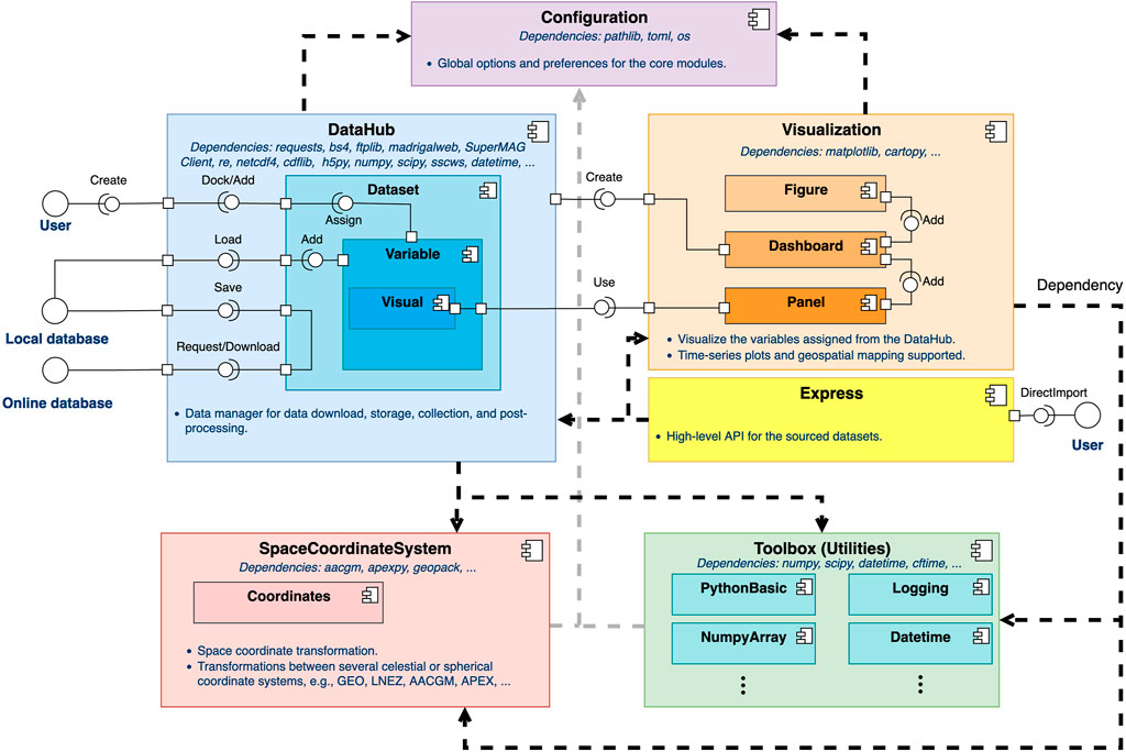
FIGURE 1. A UML component diagram showing the core modules of GeospaceLAB and their interdependence.

In the space physics community, many Python packages have been developed during the last decade for data access and analysis (e.g., Burrell et al., 2018, for a recent review). GeospaceLAB uses several useful packages for building the core modules, including CDFLIB7 for the reading/writing Computable Document Format (CDF) files, MadrigalWeb8 and SuperMAG Client for accessing Madrigal and SuperMAG databases, respectively, SSCWS9 for satellite orbit tracking, AACGMV210 (Shepherd, 2014), GEOPACK11 (Tsyganenko et al., 2021), and APEXPY12 (Richmond, 1995; Emmert et al., 2010) for coordinate system transformation.

Thanks to the existing packages, GeospaceLAB can complete multiple tasks that are required for a scientific data analysis. GeospaceLAB integrates the needed functionality of the dependencies, such that the users do not need to have a detailed knowledge of all dependencies. However, some knowledge about Python basics and the packages such as Numpy, SciPy, and Matplotlib will help the users to understand the data structure and workflows in the package.

In this paper, we present the current public release (v0.5.2) of GeospaceLAB. We introduce the design of GeospaceLAB’s core modules and their functionality in Section 2. We present a few possible applications of the package in space physics research in Section 3. The current status, issues and future plans are described in Section 4. This paper is not intended to provide a detailed documentation of the package, but is rather intended to give an overview of the functionality and design. A full documentation of the package can be found online13.

2 Software design

The modular design is applied in the development of GeospaceLAB. The package is composed of six core modules, including DataHub (geospacelab.datahub), Visualization (geospacelab.visualization), Express (geospacelab.express), SpaceCoordinateSystem (geospacelab.cs), Toolbox (geospacelab.toolbox), and Configuration (geospacelab.config). Figure 2 shows the component diagram generated in Unified Modeling Language (UML) (Engels et al., 2000) for the six core modules. The diagram describes briefly the structure of the package and the relationship among the core modules. DataHub is the data manager in GeospaceLAB. This module is used to control the workflow when processing data and to manage the data and its properties from various data sources. Visualization controls the plotting process for the data managed by DataHub. As shown in Figure 1, users should first create a DataHub or Dashboard object for the research project. In case of a DataHub object, users can dock/add one or more dataset objects. A dataset object is a collection of variables which are loaded from data files. The dataset object also controls the procedure of downloading, storing, loading, and post-processing of a specific data product. Users can make publication-quality plots using the Dashboard object. Express contains several high-level interfaces based on DataHub and Visualization. With the high-level interfaces, users can directly obtain data and view quicklook plots from a specific data source. SpaceCoordinateSystem manages the coordinate transformation to commonly used space coordinate systems. Toolbox is a library of functions that supports other modules in GeospaceLAB. Both SpaceCoordinateSystem and Toolbox support the workflows in DataHub, Visualization, and Express. Finally, Configuration manages the preferences and global parameters used in the package. In the following subsections, we will introduce the core modules in more detail.

FIGURE 2

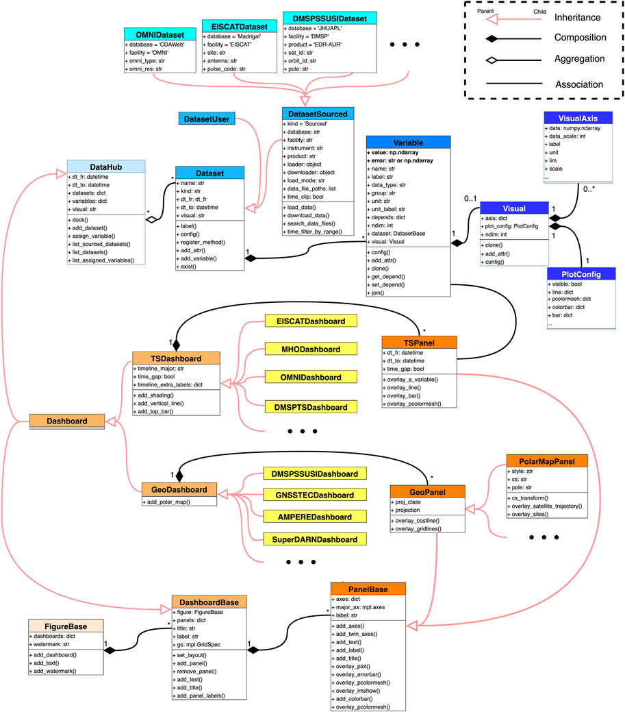
FIGURE 2. A UML class diagram that describes the main structure of the three core modules DataHub (blue color shades), Visualization (orange), and Express (yellow) in GeospaceLAB.

2.1 DataHub as the data manager (geospacelab.datahub)

DataHub is the most essential module in the package. The module is composed of several base classes and their subclasses. Figure 2 shows the main structure of the modules DataHub, Visualization, and Express in a UML class diagram. The classes included in the module DataHub are marked by blue shades. Each class is illustrated with three compartments: the upper compartment shows the name of the class, the middle contains the attributes, and the lower contains the methods owned by the class. Note that the attributes and methods of a class are not fully listed in figure. A full description can be found in the online documentation.

In the family of DataHub classes, DataHub (with the same name as the module), Dataset, and Variable are the three core classes. The class DataHub is the top-level manager that governs the global properties and behavior of a project and the dataset objects that are included. The class Dataset is the middle-level manager that controls the workflow for a specific data product and manages the data variables in that data product. The class Variable is the base-level manager that manages a specific data variable and its own properties in a data product. A DataHub object can be compared with the core module of a modular space station. It can dock or add one or more Dataset objects like a space station core module docks different types of modules. Each Dataset object owns multiple Variable objects, just like various devices in a space station module.

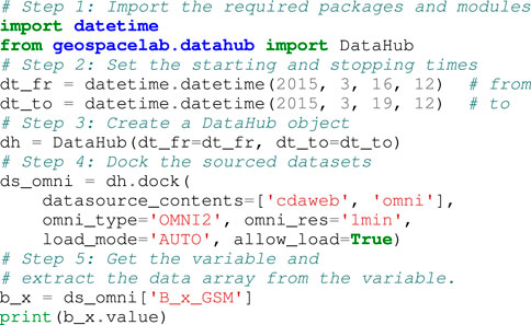
Listing 1 shows a code example with comments to help users to understand the basic workflow in using a DataHub object. The code retrieves OMNI data using five steps by 1) importing the required module, 2) setting the time bounds (dt_fr and dt_to), 3) creating a DataHub object (assigned to dh), 4) docking the OMNI dataset with several inputs (assigned to ds_omni), and 5) getting a variable from the docked dataset (assigned to B_x) and extracting the data array from B_x.value. Only a few inputs (keyword arguments) are required in steps 3 and 4. The OMNI dataset object ds_omni is responsible for the query and retrieval of the OMNI data product. The OMNI data will be downloaded automatically, if the data files do not exist in the local directory of a user’s computer. The above five steps are the standard procedures for users to obtain the data from one or more data sources. The code is simple, benefiting from the functionality of the three core classes and their inheritances.

Listing 1. An example code with comments for retrieving OMNI data from 1200UT on 16 March 2015 to 1200 UT on 19 March 2015. The data array of the interplanetary magnetic field (IMF) B_x component is printed in the final.

2.1.1 Variable

To demonstrate the framework of the data management in DataHub, first we introduce the core class Variable which is the base-level manager. In space physics, a variable from observations or simulations is often expressed or recorded by a numeric array with associated properties. The variable properties include the name, unit, description, dependencies, and errors. The class Variable provides a data model to record both data array and common properties for a physical quantity. Meanwhile, additional properties can be added flexibly when needed.

The most commonly used attributes of a Variable object have been listed in Figure 2, including value, ndim, error, name, label, data_type, group, unit, unit_label, depends, and visual. The attribute value is used to record a data array in the format numpy.ndarray. A data array may have one or more dimensions. The attribute ndim returns the number of dimensions. The attributes name, unit, data_type, group record the basic properties of a variable as described in the attribute names. The attributes label and unit_label usually have the form of a Python raw string for the text rendering with mathematics expression. They are useful when shown with the plots.

Frequently, the measurement/calculation errors are provided with the data array in space sciences. The attribute error is used to record these error values. The attribute can be assigned with either the numpy.ndarray object or a string (Python str object). In case of the string, the string value points to the error variable stored in the associated dataset object.

Any data arrays in space sciences should depend on one or more support data along a specific axis. The support data usually indicates the time, spatial position or any quantity indirectly connected to the measurement/calculation. For example, the Variable object B_x in Listing 1 is assigned by an 1-dimensional (1-D) array of the IMF B_x component with associated properties. The array depends on the universal time (UT) along the axis-0 (0 denotes the first dimensional axis, 1 the second, and 2 the third hereafter). Sometimes, a variable may have multiple dependencies along one axis. For instance, the electron density measured from a low-earth-orbit (LEO) satellite is a 1-D time-series variable, which depends on UT, geographic latitude and longitude, and geomagnetic latitude and longitude along the axis-0. The attribute depends manages the dependencies of the variable in multiple dimensions and multiple dependencies along one dimensional axis. A Variable object uses the methods set_depend () and get_depend () to set up and obtain the dependencies, respectively. Similar as error, the values of dependencies in depends can be assigned with a numpy.ndarray object or a string. In case of a string, the string value points to the supporting variable stored in the associated dataset object.

In case that a visualization is needed, the attribute visual will be assigned with a Visual object (see also Figure 2). Note that by default, the DataHub object sets its attribute visual with the value of “off”, meaning that the Visual objects will not be assigned to all variables. The class Visual manages the visualization properties for a variable with two compositions: VisualAxis and PlotConfig. A VisualAxis object controls data and options along a specific axis when plotting. Hence, one Visual object may have multiple VisualAxis objects, which are assigned to the Visual attribute axis. In addition, one Visual object owns one PlotConfig object, which controls the plotting type and the corresponding configuration.

In practice, it is not necessary to set all the attributes when creating or using a Variable object. For a sourced dataset (see Section 2.1.2.1), the attributes have been assigned as default properties for a specific variable in the data product. On the other hand, the various attributes of Variable and Visual let users or developers customize as much as possible if the default settings do not suit their needs. The method config () is used to set the multiple attributes that have been included in the classes, and add_attr () to add additional attributes if needed. The same methods are also used for the Dataset objects as described next.

2.1.2 Dataset

The class Dataset is the middle-level manager in the module DataHub. It manages a collection of data variables and the global attributes in a data product. A Dataset object is a Python dictionary-like (dict) object, in which the keys are the variable name in the type of str, and the values are the correspond Variable objects. The Dataset object owns several basic attributes, such as name for the name of the dataset, kind for the type of the dataset (see also DatasetSourced and DatasetUser below), dt_fr for the starting time, dt_to for the stopping time, and visual for determining if the Visual objects are appended to the Variable objects. The Dataset also owns a series of methods, such as add_variable () for adding a Variable object, label () for automatically generating an identical label, config () and add_attr for configuring the attributes, and register_method () for adding an external method to the Dataset object.

The class Dataset has been extended into two subclasses (inheritances): DatasetSourced and DatasetUser. The inheritance means that the subclass owns the attributes and methods of its parent class. At the same time, the subclass has its private methods, which cannot be accessed by the parent class. The use of the inheritance is convenient for users and developers to reuse, extend, or to modify the attributes and behaviours in the parent class.

2.1.2.1 Managing a sourced dataset

The subclass DatasetSourced is designed to manage the data from a specific data source (so called sourced dataset) that have been included in the package. Besides the attributes of Dataset, DatasetSourced has its own attributes for identifying the properties of the specific data source, e.g., database, facility, instrument, and product. It also owns particular methods for managing the procedures of downloading, storing, and loading data, such as load_data (), download_data (), and search_data_files () (see also Figure 2).

In DataHub, each sourced dataset has a corresponding subclass of DatasetSourced. As shown in Figure 2, the class OMNIDataset inherits from DatasetSourced with the assigned attributes database = “CDAWeb” and facility = “OMNI”. Similarly, EISCATDataset, DMSPSSUSIDataset and many other subclasses have been developed for the sourced datasets. Each subclass uses the attributes and methods of DatasetSourced as the abstracts and has its own functionality.

Figure 3 shows the main process of querying, downloading, storing, and loading data by a DatasetSourced or its subclass object. The DatasetSourced object provides three modes to load a sourced dataset: “AUTO”, “dialog”, and “assigned”. One of the values is assigned to the DatasetSourced attribute load_mode (see also Figure 2). For the mode “AUTO”, the DatasetSourced object try to finish the entire process shown in Figure 3 automatically. First, it searches the associated data files that have been stored in the local directories. This procedure is managed by the method search_data_files (). The method provides a solution to collect all data files within the time bound between dt_fr and dt_to by identifying the string patterns in the file names. The rules for the string patterns are usually defined in the specific dataset class. As a result, the data arrays that are finally loaded in the dataset are independent of how many segmented files are included. If the associated data files are not found in the local directory, a downloading procedure will be activated. The downloading procedure is implemented by a Downloader class appended to DatasetSourced. The Downloader object will search the requested files in the online database. If the files exist, the object will download the files to the local directory/database. Again, the method search_data_files () will be called to collect those downloaded files and activate the loading procedure. Similar as the downloading procedure, the loading procedure is implemented by a Loader class appended to DataSourced. The Loader object will load data and metadata from the local files and pass them to the DatasetSourced object. The DatasetSourced object will first add the queried variable objects and assign the default attributes to those objects. Then the DatasetSourced object will assign the data arrays and associated metadata to the corresponding variable objects. Finally, several post-processing procedures may be done according to the input options, such as a time filter for clipping the data within the time bound, adding additional support data, making coordinate transformation, and controlling the data quality.

FIGURE 3

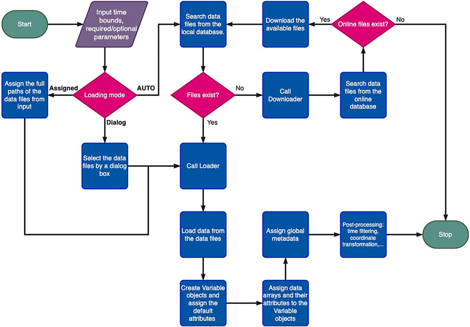
FIGURE 3. A flowchart showing the main process of downloading, storing, and loading data managed by a DataSourced object.

In GeospaceLAB, we aim to accomplish automatic downloading for most of the sourced datasets from online databases. For example, the package Requests is used for grabbing data from Hypertext Transfer Protocol (HTTP) web service, Ftplib for File Transfer Protocol (FTP) server, and several specialized packages/scripts provided by individual data services (e.g., MadrigalWeb and SuperMAG Client). We developed a family of Downloader classes to communicate with different online databases. Those sourced datasets with the same downloading mechanism can share one Downloader class. Alternatively, only a minor modification is applied by subclassing the parent Downloader class.

A similar arrangement for the Downloader classes is also applied for the family of Loader classes. So far, we have developed the Loader classes for loading data files with several kinds of formats, such as ASCII, CDF, NetCDF, HDF5, and binary files. Again, those Loader classes are highly reusable or extendable for various sourced datasets.

In case that the sourced dataset is not downloadable or only the local data files are available, users can utilize the loading modes “dialog” and “assigned’ to select the local data files. When “dialog’ is set, a dialog box will be activated. For the “assigned’ mode, users can assign the full paths of the data files to the attribute data_file_paths of the DatasetSourced object.

So far, GeospaceLAB (current version: v0.5.2) supports more than twenty kinds of sourced datasets from nine databases. Table 1 lists those datasets with the associated properties. Most of the datasets can manage the procedure of automatically downloading (“Downloadable” is True). For a few datasets that are not downloadable, the users can download the data manually from the online services, e.g., the SuperDARN electric potential map data in the ASCII format and the AMEPRE Field-aligned current maps in the NetCDF format, or request from the data provider, e.g., the GITM model results from the research group at University of Texas, at Arlington (UTA). The data in all the listed datasets are be collected continuously within the input time bound. Even if the data is stored in separate files, the associated DatasetSourced object can detect and collect all associated data files automatically. Several datasets own their high-level dashboards for directly visualizing the data. Those dashboards are importable from the core module Express (see Section 2.3).

TABLE 1

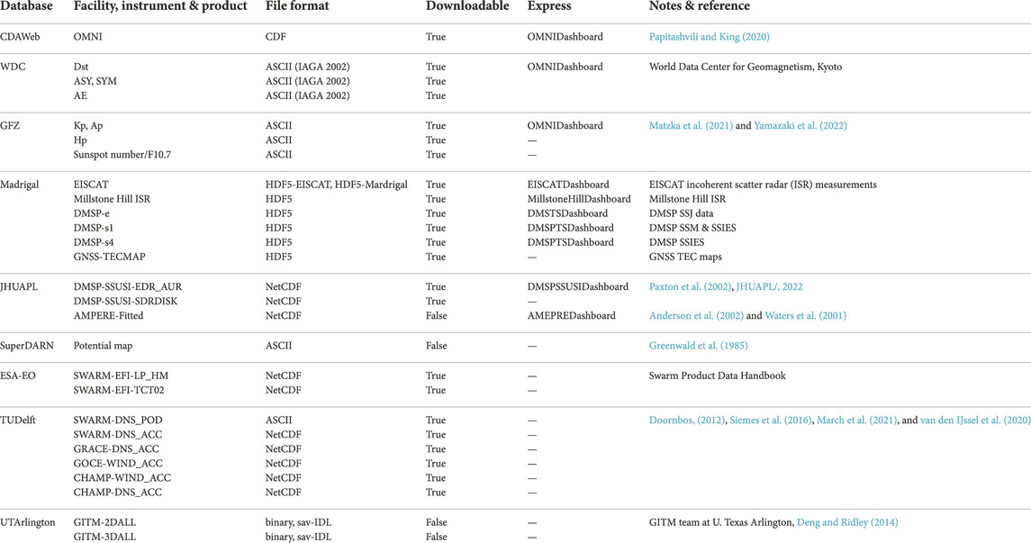
TABLE 1. A list of data sources that have been included in GeospaceLAB (Current version: v0.5.2).

2.1.2.2 Managing a user-defined dataset

In addition to DatasetSourced, the subclass DatasetUser of Dataset is designed for a user-defined dataset that has not yet been supported by GeospaceLAB. With DatasetUser, users can add data that they have downloaded and loaded using their own scripts. Users can also build a subclass of DatasetUser to customize the attributes and methods. A DataHub object has the method add_dataset () to add a DatasetUser object. As a result, a user-defined dataset can be processed together with other datasets. This is useful when users want to use the functionality of GeospaceLAB to visualize or analyze the data that has not been supported by the package. An example code14 on how to add a user-defined dataset to a DataHub or Dashboard object can be found in the GitHub repository.

2.1.3 DataHub

The class DataHub is at the top-level in the three core classes. A DataHub object owns the attributes such as dt_fr, dt_to, and visual as the global settings. Those attributes are passed to the datasets being added. The DataHub object uses the method dock () to add a DatasetSourced object (as shown in List 1), or the method add_dataset () to add a DatasetUser object. For the method dock (), the required keyword arguments can be checked by the DataHub method list_sourced_datasets () or by the online documentation.

In summary, the module DataHub provides a framework of managing data from measurements or simulations. The module manages not only the data arrays but also the associated properties. The functionality of the core classes makes it easy to integrate multiple data products with different dependencies and properties in one project. Also based on DataHub, the following modules Visualization and Express can implement a quick integration of multiple data in one figure, which helps users to view space physics events in different aspects.

2.2 Visualization (geospacelab.visualization)

2.2.1 Base classes and inheritances

With the module Visualization we aim to make publication-quality figures using data and metadata provided from DataHub. Currently, the module supports generating static plots by wrapping the matplotlib objects. The module is composed of three base classes (FigureBase, DashboardBase, and PanelBase) and a series of subclasses (see the classes marked by orange shades in Figure 2). The class FigureBase is the top level container for all plotting elements. The class is an inheritance of matplotlib.figure.Figure. Thus, the same attributes and methods used in matplotlib.figure.Figure can be set and get from FigureBase. FigureBase contains the method add_dashboard (), so that users can add one or more dashboards (defined below) to the figure object. In addition, users can add watermarks on the figure if needed.

The class DashboardBase is the second level container. A dashboard is composed of one or more panels. The method set_layout () of a DashboardBase object is used to set the dashboard’s position in a figure and to arrange the panels by rows and columns. DashboardBase owns the methods such as add_text () and add_title () to add text to the dashboard coordinates.

The class PanelBase is the base level container. The class wraps matplotlib.axes.Axes and adds additional functionality. A PanelBase object has one major ax for plotting. Several supporting axes can be added by the method add_axes () for making the colorbar, legend box, and other purposes. Like DashboardBase, PanelBase owns the methods such as add_text (), add_label (), and add_title () to add text in a panel coordinate instead of a dashboard coordinate.

From DashboardBase and PanelBase, a series of dashboards and panels have been developed (see also Figure 2). First, the class Dashboard inherits from both DataHub and DashboardBase. Hence, a Dashboard object can be used as a data manager (DataHub object) to add various datasets. Meanwhile, the class contains all functions from DashboardBase. Second, the module Visualization is currently focusing on two kinds of data: time-series data and geospatial data. Hence, two groups of dashboard and panel classes have been developed for making the time-series and geospatial mapping plots, respectively.

Using those classes, we can build a figure with multiple dashboards and panels for viewing various data simultaneously. Figure 4 shows a schematic diagram as an example of a figure with a complex layout. The figure is equivalent to a FigureBase object. It contains three dashboards (Dashboard objects). The position of each dashboard is controlled by the Dashboard method set_layout (). On the top, there is one geospatial dashboard (GeoDashboard object) with two geospatial panels (GeoPanel objects). On the bottom there are two time-series dashboards (TSDashboard objects) on the left and right sides, respectively. Each time-series dashboard contains several time-series panels (TSPanel objects). Using GeospaceLAB, users can create such figures with complex layouts in a simple and quick way.

FIGURE 4

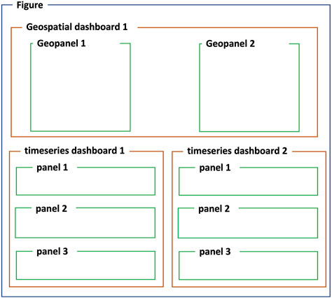
FIGURE 4. A schematic diagram as an example of a figure with a complex layout.

2.2.2 Visualizing time-series data

In space physics, most of the observational and simulation data depends on time. Even an image or a map is typically associated with a time. To view the time-series data, we have developed the subclass TSDashboard from Dashboard. Due to the inheritance, TSDashboard can also be used as a data manager (DataHub) to dock/add datasets.

The code in Listing 2 creates a TSDashboard object, which is used to retrieve and view OMNI data and additional geomagnetic indices instead of using the DataHub object as shown in Listing 1. The TSDashboard object generates a dashboard with multiple panels to show the time-series plots. The panel layouts, including the number of panels and the variables that will be plotted in one panel, are configured by calling the method set_layout () with the keyword argument panel_layouts. The plotting types, such as 1-D lines, points, error bars, and 2-D surfaces will be automatically detected, when the method draw () is called. Then the corresponding dashboard will be generated. For a sourced dataset, the plot property of a 1-D or a 2-D time-series variable have been preset. Hence, users only need to set the panel layouts by one-line command to make a free arrangement of panels and plots.

Listing 2. A code example for obtaining and visualizing OMNI and geomagnetic index data from three sourced datasets. The dashboard generated by this code is shown in Figure 5D.

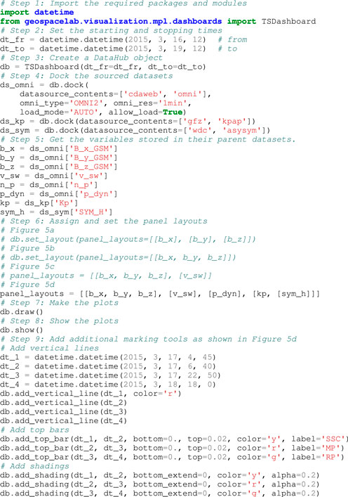
Figure 5 shows four time-series dashboards (a–d) corresponding to the code in Listing 2. Only the keyword argument panel_layouts is assigned with four different values, respectively. The assigned value is a nested Python list. The length of the outermost list indicates the number of time-series panels that will be shown in a dashboard. The element of the outermost list is a sub-list. Within the sub-list, the Variable objects that are included will be plotted in that panel. This one-line setting make it easy to add or remove panels and plots.

Additional functionalities of TSDashboard with TSPanel are listed as follows:

• Automatically adjust the time ticks and tick labels according to the time bounds assigned to dt_fr and dt_to.

• Support common 1-D and 2-D plot types like in matplotlib, including line plots, scatters, bars, pcolormesh, and image.

• Extend and customize plot types by registering new plotting function to the class TSDashboard.

• Detect and show the time gaps for regularly measured data, e.g., the blanks between some data points shown in Figure 5D top panel.

• Provide several marking tools, such as vertical lines across panels, horizontal bars, and rectangular shadings. The marking tools are often used to indicate interesting time periods for a event analysis, as shown in Figure 5D.

• Support to generate multiple lines of tick labels that indicate different support data, respectively. For example, this option is useful for viewing the satellite data depending not only on UT but also on geospatial locations simultaneously (see also Figure 9 bottom).

FIGURE 5

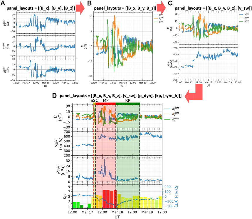
FIGURE 5. An example of using the keyword argument panel_layouts to set the panel layouts in a time-series dashboard. The keyword value determine the panel layout of a dashboard as shown in panels (A–D). In panel (D), from top to bottom are the IMF B_x, B_y and B_z components, the solar wind speed, the solar wind dynamic pressure, and Kp and SYM-H indices during the 2015 St. Patrick’s Day storm. The dashed vertical lines, shadings, top bars indicate the three phases of the storm, including the initial phase (or SSC), main phase (MP), and recovery phase (RP)¹⁵.

2.2.3 Visualizing geospatial data

Based on Dashboard, the subclass GeoDashboard is used for viewing the geospatial data. A GeoDashboard object uses the method set_layout () to arrange the GeoPanels (GeoPanel objects) in multiple rows and columns. The class GeoPanel inherits from PanelBase and wraps the “GeoAxes” of the package cartopy. As a result, users can make most types of map projections in cartopy by adding the GeoPanel object to the GeoDashboard object.

The map projections in cartopy use the geographic (GEO) coordinate system. However, in many space physics studies, especially when examining the magnetosphere-ionosphere-thermosphere (M-I-T) coupling, a geomagnetic coordinate system is used, because the geomagnetic field plays an important role in governing the dynamics and electrodynamics in the M-I-T system. To solve the mapping projections in a geomagnetic coordinate system, a subclass of GeoPanel has been developed, so called PolarMapPanel.

Using PolarMapPanel, users can project the 1-D or 2-D geospatial data on the polar map in three view styles: 1) polar projection with the geographic latitude/longitude (GLON-fixed), 2) polar projection with geographic latitude and local solar time (LST-fixed), and 3) polar projection with geomagnetic latitude and magnetic local time (MLT-fixed). The polar projection is based on the stereographic projection method. The class PolarMapPanel supports mapping in several geomagnetic coordinate systems, such as Altitude Adjusted Corrected Geogmagnetic Coordinates (AACGM), Magnetic Apex Coordinates (APEX), and Quasi-Dipole coordinates (QD) (see also Laundal and Richmond, 2017). The coordinate transformations are supported by the module SpaceCoordinateSystem.

Figure 6 shows an example of the GNSS TEC maps in the three view types at 0620 UT on 17 March 2015 during the St. Patrick’s Day storm. The coastlines, grid lines and labels can optionally be added in all three views, which helps users to identify and pinpoint interesting structures and their locations in the polar maps (see the discussion in Section 3.2).

FIGURE 6

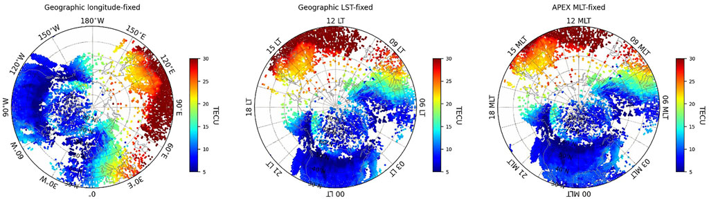
FIGURE 6. An example of the polar maps showing the GNSS/TEC in the northern hemisphere at 0620 UT on 17 March 2015 during the SSC of the 2015 St. Patrick’s Day storm in three view modes: left—fixed at the geographic longitude of 0°, middle—fixed at the solar local time (SLT) of 0 o’clock, and right—fixed at 0 MLT in the APEX coordinate system¹⁶.

In summary, a PolarMapPanel can be used to:

• Show polar maps in three view styles: GLON-fixed, LST-fixed, and MLT-fixed.

• Utilize optional geomagnetic coordinate systems, so far AACGM, APEX, and QD are included.

• Add coastlines in either a geographic or a geomagnetic coordinate system.

• Add latitude and longitude grid lines and their labels.

• Support basic 1-D or 2-D plots provided by matplotlib and cartopy.

• Overlay satellite trajectories with time ticks and tick labels (see nine top).

• Overlay satellite cross-track vectors along the satellite trajectory (see nine top).

• Mark ground-based sites on the polar map (see nine top).

• Re-sample or re-grid data for proper mapping.

In addition to PolarMapPanel, other subclasses of GeoPanel are currently under development. Several more types of map projections will be added for both global and regional mapping in the future.

2.3 Express (geospacelab.express)

The module Express contains a number of high-level dashboards developed from TSDashboard or GeoDashboard. Those dashboard classes are shown in Figure 2 with yellow shades. A set of classes inherit from TSDashboard, including EISCATDashboard, MHODashboard, OMNIDashboard, and DMSPDashboard. The class names have indicated the purposes. They are used for viewing time-series plots for the variables from specific datasets (EISCAT, Millstone Hill Observatory, OMNI, DMSP, respectively). Users only need a few input to get the data and make a quicklook figure.

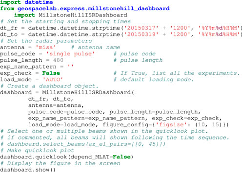
The code in Listing 3 is used to generate a quicklook dashboard for the ionospheric parameters measured by the Millstone Hill incoherent scatter radars during the 2015 St. Patrick’s Day storm from 12 UT on 17 March 2015 to 12 UT on 19 March 2015. By importing the high-level dashboard MillStoneHillISRDashboard, only a few lines of code can generate a quicklook dashboard. The output dashboard is shown in Figure 7A. The dashboard contains five panels. From top to bottom are altitude versus UT variations for 1) electron density, 2) electron temperature, 3) ion temperature, 4) line-of-sight ion velocity, as well as 5) the radar parameters.

FIGURE 7

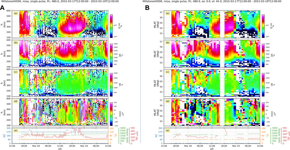
FIGURE 7. An example of two quicklook figures generated from MillstonHillDashboard in Express, which shows the Millstone Hill incoherent scatter radar measurements during the 2015 St. Patrick’s Day storm. (A): Measurements from the steerable antenna MISA with multiple scanning beams. (B): Measurements from the same radar, but only one beam selected with the az = 0° (azimuth angle) and el = 45° (elevation angle)¹⁷.

Listing 3. A code example for generating a quicklook dashboard of Mill Stone Hill measurements during the 2015 St. Patrick’s Day storm from 12 UT on 17 March 2015 to 12 UT on 19 March 2015.

The dashboards in Express are also used to add customized functionality for a specific dataset. For example, the dashboards like EISCATDashboard and MillstoneHillDashboard provide methods to check the beam directions of a radar antenna. In case of a steerable antenna, the radar experiment is often made with a multi-beam scanning mode. To check and select beams, several particular methods have been developed. As shown in Figure 7B, the dashboard shows five panels in the same format as on the left, but with the selected beam with az = 0° and el = 45°. To generate this quicklook dashboard, users only need to uncomment the line with dashboard.select_beams () in the code in List 3.

In addition, Figure 7B shows the ionospheric parameters as a function of the AACGM MLAT instead of the altitude along the y-axis. The configuration is implemented by making a minor modification of the attributes in the Visual object appended to the corresponding Variable object.

2.4 SpaceCoordinateSystem (geospacelab.cs)

In space physics research, establishing a proper coordinate system and frame of reference helps us to simplify a given problem and to better understand the underlying physical processes. A variety of coordinate systems and frame of references exists which are widely used (see the reviews by Hapgood (1992), Laundal and Richmond (2017); Shi et al. (2019)). Several python packages have been developed for coordinate system transformations, e.g., AACGMV2, APEXPY, GEOPACK, and IGRF (Michael, 2021). Those packages are widely used, however, the functions from different packages are called in different ways and the outputs have different data structures. The module SpaceCoordinateSystem aims to provide a unified interface for the coordinate transformation among different coordinate systems. The module wraps those popular packages and develops coordinate system classes based on two base classes: SpaceCSBase and CoordinateBase.

Figure 8 shows the UML class diagram of the module SpaceCoordinateSystem. The base class CoordinateBase manages a collection of coordinates in a specific coordinate system. SpaceCSBase abstracts the functions for the coordinate transformation. A SpaceCSBase object represents a coordinate system, which is appended with one CoordinateBase object recording the coordinate data.

FIGURE 8

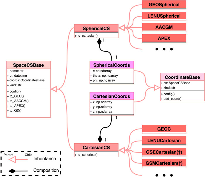
FIGURE 8. A UML class diagram that describes the main structure of the module SpaceCoordinateSystem in the same format as in Figure 2. The classes marked by * are under development.

Based on those two classes, two groups of classes have been developed: one group for spherical coordinate systems and the other for Cartesian coordinate systems. So far, the classes for spherical coordinate systems include GEOSpherical, LENUSpherical, AACGM, and APEX. The classes for Cartesian coordinate systems include GEOC, LENUCartesian, GSECartesian, and GSMCartesian. The name LENU refers to the local east-north-upward coordinate system fixed at the Earth’s surface. Those classes use unified commands to achieve the coordinate transformation. For example

cs_LENUC = cs_LENUS.to_cartesian ()

cs_GEO = cs_LENUC.to_GEO ()

where the arguments cs_LENUC, cs_LENUS and cs_GEO are the objects of LENUCartesian, LENUSpherical, and GEOSpherical, respectively. The coordinate transformations are completed by calling the functions with the same structure. The coordinate data stored in those objects also have the same data structure.

The module SpaceCoordinateSystem supports the modules such as DataHub, Visualization, and Express in case a coordinate transformation is needed. On the other hand, users can use the functionality provided by SpaceCoordinateSystem for their own codes. For this purpose, an example code19 is provided in the GitHub repository.

2.5 Toolbox (geospacelab.toolbox)

The module Toolbox is built mainly with a function-oriented design. The module is composed of several sub-modules. Each sub-module contains a series of functions. Figure 1 lists four commonly used sub-modules in Toolbox, including:

• PythonBasic: provides the utility functions associated with the basic data types in Python, such as numerical number, list, str, and dict.

• Logging: provides a customized logging system for tracking the events that occur when the package runs.

• NumpyArray: provides the utility functions associated with numpy arrays.

• Datetime: provides the utilitarian functions for the date and time, including convert time between different formats (such as unix_time, datetime, and MATLAB datenum) and supplementary functions for datetime.

2.6 Configuration (geospacelab.config)

The module configuration contains the class Preferences to manage the global settings in the package. Users can customize the global settings either temporally or permanently, based on the method set_user_config () of Preferences. For example, a basic configuration is needed, when the GeospaceLAB package is imported for the first time after installation. The configuration is to set the default root directory that stores the data downloaded by the sourced dataset classes. In addition, when accessing the Madrigal online database, it will ask for inputs of the user’s full name, email, and affiliation as cookies. The module Configuration also manages the cookies, so that users do not need to input those cookies every time when accessing the Madrigal database.

A configuration file in the toml format is used to record the users’ default settings. The file can be found at “ [USER_HOME_DIRECTORY]/.geospacelab/config.toml”. Users can modify the default settings recorded in the file. The new settings will be automatically loaded when the package is imported the next time.

In the current version (v0.5.2), the Preferences object is used only to set several key parameters. However, with increasing functionality of the package, users may need to control more global settings for the modules and functions. For this purpose, the class Preferences provides a frame to configure the global settings and it can be easily extended in future.

3 Applications

The core modules make GeospaceLAB suitable for managing and visualizing various data sets in space physics. Users can directly use the sourced datasets listed in Table 1 for their research projects. The number of the sourced datasets will increase in the future.

Currently, the sourced datasets include data from ground-based measurements (e.g., EISCAT, Millstone Hill incoherent scatter radars and SuperDARN), satellite measurements (e.g., DMSP, SWARM, and Grace), simulations (GITM), and various solar and geomagnetic activity indices (e.g., F10.7, Kp, Ap, Dst, ASY/SYM, and AE). Those datasets are typically used in magnetosphere-ionosphere-thermosphere coupling studies. A few examples are given in the following subsection. These are chosen to illustrate the capabilities of GeospaceLAB, but do not aim at a detailed scientific analysis of the events.

3.1 Space weather events

Users can search and study space weather events by combining solar wind and geomagnetic activity index data in a dashboard. For example, Figure 5D (see also Section 2.1.2.1) shows a space weather event during the St. Patrick’s Day in 2015. This famous St. Patrick’s Day storm has been studied in a number of papers (e.g., Astafyeva et al., 2015; Wu et al., 2016; Zhang et al., 2017, and references therein). Figure 5D, shows an interplanetary coronal mass ejection (ICME) arriving at the Earth’s magnetospause at about 0445 UT on 17 March 2015, which is associated with an enhanced magnetic field strength in the top panel, a sudden increase in the solar wind velocity (second panel) and an enhancement in the dynamic pressure (third panel). The interaction between the ICME and the Earth’s magnetosphere causes a strong geomagnetic storm. The SYM-H index shown in the bottom panel can be used to identify the storm phases. The sudden storm commencement (SSC) (also referred as the initial phase) is the time period with positive SYM-H (in this case between 0445 and 0640 UT on 17 March 2015) the main phase (MP) starts when the SYM-H index turns negative (in this case at 0640 UT) and the main phase ends and the recovery phase (RP) begins, when the SYM-H index has reached its minimum value (in this case at 2250 UT). Finally, when the SYM-H index recovers, the recovery phase ends (in this case at 1800 UT on 18 March 2015). Users can easily mark the storm phases using the marking methods provided by the class TSDashboard, including vertical lines, shadings, and topbars.

3.2 Global view of the key parameters in the ionosphere-thermosphere system

GeospaceLAB contains classes such as GeoDashboard and GeoPanel for visualizing geospatial data. To understand the physics behind ionospheric features, it is often necessary to study 2D-maps in geomagnetic rather than geographic coordinates, as the ionospheric coupling with the solar wind is guided by the geomagnetic field. A geographic view is on the other hand often necessary, e.g., to be able to examine whether a ground-based station is located in the proximity of an interesting ionospheric feature. However, online datasets often provide data only in geographic coordinates. The class PolarMapPanel inheriting from GeoPanel can be used for mapping 1-D or 2-D data in a polar map with either geographic or geomagnetic coordinates.

Figure 6 (discussed in Section 2.2.3), shows the global distribution of the total electron content (TEC) derived from the GNSS network at 0620 UT during the SSC of the 2015 St. Patrick’s Day storm. With the help of the global maps, the researchers can identify both large- and meso-scale structures in a 2-D TEC map. For example, the maps show the typical large-scale distribution of the TEC from dayside to the nightside due to solar radiation. In addition, a mid-latitude trough is seen over North America, extending from the evening sector to the post mid-night sector. Using GeospaceLAB, it is also feasible to overlay additional layers on the top of the TEC maps for a comparison across multiple types of data, e.g., a contour plot of the electric potential measured by SuperDARN or cross-track vectors along a satellite trajectory.

3.3 Regional or local responses

The sourced datasets include local measurements from an individual ground-based instrument or in situ measurements along a satellite trajectory. To view the local ionospheric/thermospheric responses, the TSDashboard and TSPanel described in Section 2.2.2 are often used.

As shown in Figure 7, the Millstone Hill incoherent radar measured several basic plasma parameters in the ionosphere during the MP and RP of the 2015 St. Patrick’s Day storm. The measurements show a strong enhancement of the electron density in the F-region at around 1800 UT on 17 March 2015 during the MP. This enhancement is identical and associated with the storm-enhanced density (SED) in the mid-latitude ionosphere (Zhang et al., 2017).

The two dashboards shown in Figure 7 are generated by the high-level dashboard object in the module Express for a quicklook view. Again, users can make more customized plots by using the lower-level TSDashboard class.

3.4 Conjugate satellite observations

The module Visualization gives the flexibility to arrange multiple dashboards and panels in one figure (see e.g., Figure 4), and to combine conjugate satellite observations and integrate these in a single figure.

Figure 9 shows an event with near-simultaneous measurements from the DMSP and SWARM A/C satellites above the northern auroral oval. The layout of the figure corresponds to that shown in Figure 4. On the top is the geospatial dashboard composed of two polar maps. The polar maps show the DMSP SSUSI auroral images in the LBHS wavelength band, overlaid with the trajectories of the two satellites and the cross-track velocities measured by the DMSP F18 satellite. In addition, two EISCAT incoherent scatter radar sites in Tromsø and on Svalbard, Norway are marked with black triangles on the maps.

FIGURE 9

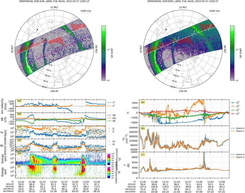
FIGURE 9. Measurements from the DMSP and SWARM satellites around 1256 UT on 17 March 2015. Top-left: DMSP/SSUSI EDR-AUR auroral image in the LBHS band overlaid with both DMSP (white) and SWARM-A/C (magenta) trajectories, top-right: DMSP/SSUSI EDR-DISK image in the same format as the top-left, bottom-left: DMSP SSIES, SSJ, and SSM measurements along the trajectory shown in top panels, and bottom-right: SWARM A and C measurements of electron density, electron temperature, and cross-track and ram velocities along the trajectory shown in the top panels. This figure shows a complex layout corresponding to Figure 4.¹⁸

This example shows an interesting event of a large-scale transpolar arc (TPA) (Kullen, 2012; Hosokawa et al., 2020) appearing in the middle of the polar cap during the main phase of the 2015 St. Patrick’s Day storm. Both, the DMSP F18 and the SWARM A/C satellite crossed the northern hemisphere from the duskside to the dawnside almost at the same time. The two satellites measured the ionospheric parameters of the TPA at two locations: DMSP F18 was close to the dayside tip of the TPA and SWARM A/C across the main part of the TPA.

The in situ measurements of the DMSP F18 satellite are shown in the time-series dashboard on the bottom-left side, and the Swarm A/C measurements are shown on the bottom-right side. On the bottom, time tick labels are shown with the corresponding geospatial information, including GEO/LAT, GEO/LON, AACGM/LAT, and AACGM/MLT. The additional labels help us to identify the location of the key features shown in the time-series dashboards and make it easier to compare those with the auroral structures shown in the geo-dashboard on the topside of the figure. The entire figure including image, time series plots and all labels was produced with the visualization module. Among other details, the time series reveals that the TPA lies on sunward plasma flow (top panel at 1554 UT in DMSP time-series plots and top panel at 1551 UT in SWARM time-series plots). The bottom panel of the DMSP measurements shows that the TPA is populated by plasma sheet ions, hinting on a source region on closed magnetic field lines (Kullen, 2012).

The two polar maps in Figure 9 show the same auroral structures, however, the appearances are slightly different. The left side shows SSUSI EDR-AUR data and the right side shows SSUSI SDR-DISK data. Both data products are listed in Table 1. The SDR-DISK image is a lower-level data product and the daylight dilution of the image has not been removed. The key issue in the two maps is that the EDR-AUR image on the left is slightly tilted counter-clockwise with respect to the satellite trajectory. The SDR-DISK image position is normal, parallel to the satellite trajectory as expected. The difference is plausibly caused by using a different version of the AACGM model by the data provider and GeospaceLAB. The SDR-DISK product provides image grids in the geographic coordinate system. The geographic coordinates are transformed to the AACGM coordinates by GeospaceLAB when the SDR-DISK image is mapped. However, the EDR-AUR product only includes the AACGM coordinates for the image grids. GeospaceLAB uses that AACGM grids directly to map the image. Since the former mapping with the SDR-DISK data is consistent with the mapping of the satellite trajectory, for which the coordinates are also transformed from the geographic coordinates by the module SpaceCoordinateSystem, we suggest that the version of AACGM model used by the SSUSI Team may be different from the AACGMV2 python package used in GeospaceLAB.

4 Current status and future

The GeospaceLAB project was started in 2021. The initial establishment was based on the proprietary MATLAB and Python libraries used in the authors’ own research works (e.g. Cai et al., 2021). After one and a half years of systematic development, GeospaceLAB has become stable for most of the modules and functions. The package is open-sourced with the BSD-3-Clause license and available in a GitHub repository (JouleCai/geospacelab version v0.5.2). The package is also uploaded to PyPI and can be easily installed via “pip”.

4.1 Issues and solutions

The development of GeospaceLAB is ongoing. The main structures of the core modules in the package are well established. Still, there are several known issues regarding the package itself, the package dependencies, and the data sources that would benefit from improvement or expansion. These are listed below:

• So far, the package has been developed with focus on the demands by the authors. It does not yet cover several data products, specifically data from the Earth’s magnetosphere or heliosphere.

Due to the well-designed core framework, it is feasible to include more datasets in DataHub, add more plotting routines in Visualization, and expand SpaceCoordinateSystem with more coordinate system transformation methods. To do so, additional workflows and maintenance are required. Hence, we would like to invite contributors to join this project by submitting new data products and adding new functionalities. Guidelines for advanced users and developers are available in the online documentation20.

• The first priority for GeospaceLAB is to include high-level data products from data providers. The term “high-level data” means that the data product is calibrated, qualified, or can be directly used in research studies. However, issues with the data may still occur. For example, the mapping difference between two kinds of DMSP SSUSI products is discussed in Section 3.4. We highly recommend that users should always familiarize themselves with the data definitions, formats, and usage policy from the data providers. The DatasetSourced object in GeospaceLAB has the attributes, such as database, facility, and product, which record the URL and notes of data usage for individual data products. The users can extract the information and contact the principal investigators of the data product if needed.

• The package is compatible with most of the dependent packages. However, sometimes users have reported that the package AACGMV2 returns errors when it is imported from GeospaceLAB. This happened mainly when a user used a specific integrated development environment (IDE), such as “PyCharm” or “VS. Code”. The issue can be solved, if the IDE “Spyder” is used. However, a more general solution should be implemented in future. We have reported this issue to the GitHub repository of AACGMV2.

• The package has mostly been tested in the operating systems (OS) of Ubuntu and macOS. Its compatibility with the Windows OS and other Linux distributions is not guaranteed.

We thank the users who have contributed to the GeospaceLAB project by pointing out open issues and providing feedback on GitHub. The activities have helped to improve the performance of the package.

4.2 Proposed features

Since the core modules of GeospaceLAB are easily extendable, many new features can be added to them in future releases. The next major release will be version 1.0, scheduled for the end of 2022. In version 1.0, the package will become more stable, and will include the following features:

• Extension of the sourced datasets with several commonly used data products in the community.

• A well-structured online documentation.

• Support of several new plotting styles in the Visualization module for the 1-D or 2-D data.

• Support of more coordinate system transformations in the module SpaceCoordinateSystem.

• Enhanced testing of the package to make it more robust using the Python package PyTest.

5 Summary

GeospaceLAB is an easy-to-use, extendable Python package for managing and visualizing observational and modeling data that is used in the space physics community. The package has been applied to research topics regarding the study of M-I-T coupling in the authors’ research groups. So far, the package has been downloaded from GitHub or PyPI with cumulative number of more than 28,000 times. In each released version, the number of users has been more than 50 (See also the online statistics21).

GeospaceLAB bridges data providers and scientists. It provides systematic solutions in data management, visualization, and space coordinate transformation.

• GeospaceLAB can be used as a data manager for various observational and modeling data in space physics. The data products can be obtained from external providers, e.g., an online database, or from the users’ local database. For online data, GeospaceLAB aims to achieve automatic downloading, storing, and loading of data.

• GeospaceLAB can also generate high-qualify publication-ready figures. With specialized functions and tools, the package is particularly suitable for viewing time-series and geospatial data in space physics. Users can easily combine multiple kinds of data and integrate them into one figure.

• GeospaceLAB provides a simple, unified interface for transforming from one space coordinate system to another. Currently, it can be used to switch between the geographic (GEO), geocentric (GEOC), AACGM, APEX, QD, and local east-north-upward (LENU) coordinate systems. More transformations will be added in the future.

• The functionality of GeospaceLAB described in previous sections makes it possible to advance quickly with the data analysis itself. Since a Variable object stores the data in the form of NumPy array, GeospaceLAB is compatible with most popular packages in data analysis, such as NumPy, SciPy, and Pandas. In addition, the data arrays collected by GeospaceLAB are independent of file segments. That could potentially be used for analyzing big data in collaboration with other popular Python libraries.

Since the framework in the core modules is well structured, the package is highly extendable for multiple purposes in space research. We invite members of the community to contribute to GeospaceLAB, by using the package for their research, reporting issues, proposing new functions, and joining its further development.

Data availability statement

The original contributions presented in the study are included in the article/supplementary material, further inquiries can be directed to the corresponding author.

Author contributions

LC is the principal developer of the GeospaceLAB package and wrote the manuscript. AA is the principal investigator of LC’s postdoc project and suggested the functionality of the package. AK and YD were the supervisors for LC’s former projects and provided comments on the package development. S-RZ commented on the usage of Millstone Hill ISR and GNSS TEC data. YZ commented on the usage of DMSP SSUSI data. IV and HV helped the development of the package. All co-authors contributed to the discussions and provided editorial comments on the manuscript.

Funding

The development of the GeospaceLAB package is supported by the Kvantum Institute at University of Oulu. AK and LC acknowledge postdoc grant DNR-155A/17 funded by Swedish National Space Agency. YD was supported by AFOSR through award FA9559-16-1-0364 and NASA grants 80NSSC20K0195, 80NSSC20K1786 and 80NSSC22K0061. S-RZ acknowledges MURI grant ONR15-FOA-0011 and NSF grant AGS-2033787. HV was supported by the Academy of Finland project 314664. The authors acknowledge all the developers who developed the dependencies used in GeospaceLAB. The authors also acknowledge the data providers listed in Table 1 to support the open access of data. Millstone Hill ISR observation, GNSS TEC data processing, and Madrigal database system are provided to the community by MIT under the US NSF grant AGS-1952737 support. We acknowledge use of NASA/GSFC’s Space Physics Data Facility’s OMNIWeb (or CDAWeb or ftp) service, and OMNI data.

Conflict of interest

The authors declare that the research was conducted in the absence of any commercial or financial relationships that could be construed as a potential conflict of interest.

Publisher’s note

All claims expressed in this article are solely those of the authors and do not necessarily represent those of their affiliated organizations, or those of the publisher, the editors and the reviewers. Any product that may be evaluated in this article, or claim that may be made by its manufacturer, is not guaranteed or endorsed by the publisher.

Footnotes

¹https://github.com/psf/requests.

²https://www.crummy.com/software/BeautifulSoup/bs4/doc/.

³https://docs.python.org/3/library/ftplib.html.

⁴https://docs.python.org/3/library/pathlib.html.

⁵https://github.com/Unidata/netcdf4-python.

⁶https://www.h5py.org/.

⁷https://github.com/MAVENSDC/cdflib.

⁸http://cedar.openmadrigal.org/docs/name/rr_python.html.

⁹https://sscweb.gsfc.nasa.gov/WebServices/REST/py/sscws/sscws.html.

¹⁰https://github.com/aburrell/aacgmv2.

¹¹https://github.com/tsssss/geopack.

¹²https://github.com/aburrell/apexpy.

¹³https://geospacelab.readthedocs.io/en/latest/.

¹⁴https://github.com/JouleCai/geospacelab/blob/master/examples/demo_user_defined_dataset.py.

¹⁵Source code: https://github.com/JouleCai/geospacelab/blob/master/examples/manuscript_example_2_%20omni.py.

¹⁶Source code: https://github.com/JouleCai/geospacelab/blob/master/examples/manuscript_example_4_GNSS.py.

¹⁷Source code: https://github.com/JouleCai/geospacelab/blob/master/examples/manuscript_example_3_%20isr.py.

¹⁸Source code: https://github.com/JouleCai/geospacelab/blob/master/examples/manuscript_example_5_dmsp_swarm.py.

¹⁹https://github.com/JouleCai/geospacelab/blob/master/examples/demo_cs_transform.py.

²⁰https://geospacelab.readthedocs.io/en/latest/dev/guidance.html.

²¹https://pepy.tech/project/geospacelab.

References

Anderson, B., Takahashi, K., Kamei, T., Waters, C., and Toth, B. (2002). Birkeland current system key parameters derived from Iridium observations: Method and initial validation results. J. Geophys. Res. 107, 1079. SMP–11. doi:10.1029/2001ja000080

CrossRef Full Text | Google Scholar

Astafyeva, E., Zakharenkova, I., and Förster, M. (2015). Ionospheric response to the 2015 St. Patrick’s day storm: A global multi-instrumental overview. J. Geophys. Res. Space Phys. 120, 9023–9037. doi:10.1002/2015ja021629

CrossRef Full Text | Google Scholar

Burrell, A. G., Halford, A., Klenzing, J., Stoneback, R., Morley, S. K., Annex, A., et al. (2018). Snakes on a spaceship—an overview of Python in heliophysics. J. Geophys. Res. Space Phys. 123, 10–384. doi:10.1029/2018ja025877

CrossRef Full Text | Google Scholar

Cai, L., Kullen, A., Zhang, Y., Karlsson, T., and Vaivads, A. (2021). DMSP observations of high-latitude dayside aurora (HiLDA). JGR. Space Phys. 126, e2020JA028808. doi:10.1029/2020ja028808

CrossRef Full Text | Google Scholar

Caswell, T. A., Droettboom, M., Lee, A., de Andrade, E. S., Hoffmann, T., Klymak, J., et al. (2022). Matplotlib/matplotlib: Rel: 3.5. doi:10.5281/zenodo.6513224

CrossRef Full Text | Google Scholar

[Dataset] Michael, (2021). space-physics/igrf: IGRF model. doi:10.5281/zenodo.5560949

CrossRef Full Text | Google Scholar

Deng, Y., and Ridley, A. J. (2014). The global ionosphere-thermosphere model and the nonhydrostatic processes. Model. Ionosphere–Thermosphere Syst., 85–100. doi:10.1002/9781118704417.ch8

CrossRef Full Text | Google Scholar

Doornbos, E. (2012). Thermospheric density and wind determination from satellite dynamics. Springer Science & Business Media.

Google Scholar

Emmert, J., Richmond, A., and Drob, D. (2010). A computationally compact representation of Magnetic-Apex and Quasi-Dipole coordinates with smooth base vectors. J. Geophys. Res. 115. doi:10.1029/2010JA015326

CrossRef Full Text | Google Scholar

Engels, G., Heckel, R., and Sauer, S. (2000). “UML—A universal Modeling Language?” in International conference on application and theory of petri nets (Springer), 24–38.

CrossRef Full Text | Google Scholar

Greenwald, R., Baker, K., Hutchins, R., and Hanuise, C. (1985). An HF phased-array radar for studying small-scale structure in the high-latitude ionosphere. Radio Sci. 20, 63–79. doi:10.1029/rs020i001p00063

CrossRef Full Text | Google Scholar

Hapgood, M. (1992). Space physics coordinate transformations: A user guide. Planet. Space Sci. 40, 711–717. doi:10.1016/0032-0633(92)90012-d

CrossRef Full Text | Google Scholar

Harris, C. R., Millman, K. J., van der Walt, S. J., Gommers, R., Virtanen, P., Cournapeau, D., et al. (2020). Array programming with NumPy. Nature 585, 357–362. doi:10.1038/s41586-020-2649-2

PubMed Abstract | CrossRef Full Text | Google Scholar

Hosokawa, K., Kullen, A., Milan, S., Reidy, J., Zou, Y., Frey, H. U., et al. (2020). Aurora in the polar cap: A review. Space Sci. Rev. 216, 15–44. doi:10.1007/s11214-020-0637-3

CrossRef Full Text | Google Scholar

Hunter, J. D. (2007). Matplotlib: A 2D graphics environment. Comput. Sci. Eng. 9, 90–95. doi:10.1109/MCSE.2007.55

CrossRef Full Text | Google Scholar

Jhuapl/, S. S. U. S. I. (2022). DMSP SSUSI data products. Available at: https://ssusi.jhuapl.edu/(Accessed August 19, 2022).

Google Scholar

Kullen, A. (2012). Transpolar arcs: Summary and recent results. Auror. Phenomenology Magnetos. Process. Earth Other Planets, Geophys. Monogr. Ser 197, 69–80. doi:10.1029/2011GM001183

CrossRef Full Text | Google Scholar

Laundal, K. M., and Richmond, A. D. (2017). Magnetic coordinate systems. Space Sci. Rev. 206, 27–59. doi:10.1007/s11214-016-0275-y

CrossRef Full Text | Google Scholar

Luciano, R. (2015). Fluent Python: Clear, concise, and effective programming. Sebastopol, CA, United States: OŔeilly Media.

Google Scholar

March, G., Van Den Ijssel, J., Siemes, C., Visser, P. N., Doornbos, E. N., and Pilinski, M. (2021). Gas-surface interactions modelling influence on satellite aerodynamics and thermosphere mass density. J. Space Weather Space Clim. 11, 54. doi:10.1051/swsc/2021035

CrossRef Full Text | Google Scholar

Matzka, J., Stolle, C., Yamazaki, Y., Bronkalla, O., and Morschhauser, A. (2021). The geomagnetic K_p index and derived indices of geomagnetic activity. Space weather. 19, e2020SW002641. doi:10.1029/2020sw002641

CrossRef Full Text | Google Scholar

Met Office (20102015). Cartopy: A cartographic python library with a matplotlib interface. Exeter, Devon.

Google Scholar

Papitashvili, N. E., and King, J. H. (2020). OMNI combined heliospheric observations (COHO), merged magnetic field, plasma and ephemeris, definitive hourly data. doi:10.48322/6ffx-3441

CrossRef Full Text | Google Scholar

Paxton, L. J., Morrison, D., Zhang, Y., Kil, H., Wolven, B., Ogorzalek, B. S., et al. (2002). Validation of remote sensing products produced by the special sensor ultraviolet scanning imager (SSUSI): A far uv-imaging spectrograph on dmsp f-16. Opt. Spectrosc. Tech. remote Sens. Instrum. Atmos. space Res. IV 4485, 338–348. doi:10.1117/12.454268

CrossRef Full Text | Google Scholar

Richmond, A. (1995). Ionospheric electrodynamics using magnetic Apex coordinates. J. Geomagn. Geoelec. 47, 191–212. doi:10.5636/jgg.47.191

CrossRef Full Text | Google Scholar

Shepherd, S. (2014). Altitude-adjusted corrected geomagnetic coordinates: Definition and functional approximations. J. Geophys. Res. Space Phys. 119, 7501–7521. doi:10.1002/2014ja020264

CrossRef Full Text | Google Scholar

Shi, Q., Tian, A., Bai, S., Hasegawa, H., Degeling, A., Pu, Z., et al. (2019). Dimensionality, coordinate system and reference frame for analysis of in-situ space plasma and field data. Space Sci. Rev. 215, 35–54. doi:10.1007/s11214-019-0601-2

CrossRef Full Text | Google Scholar

Siemes, C., de Teixeira da Encarnação, J., Doornbos, E., Van Den Ijssel, J., Kraus, J., Pereštỳ, R., et al. (2016). Swarm accelerometer data processing from raw accelerations to thermospheric neutral densities. Earth Planets Space 68, 92–16. doi:10.1186/s40623-016-0474-5

CrossRef Full Text | Google Scholar

Tsyganenko, N., Andreeva, V., Kubyshkina, M., Sitnov, M., and Stephens, G. (2021). Data-based modeling of the Earth’s magnetic field. Magnetos. Sol. Syst., 617–635. doi:10.1002/9781119815624.ch39

CrossRef Full Text | Google Scholar

van den Ijssel, J., Doornbos, E., Iorfida, E., March, G., Siemes, C., and Montenbruck, O. (2020). Thermosphere densities derived from Swarm GPS observations. Adv. Space Res. 65, 1758–1771. doi:10.1016/j.asr.2020.01.004

CrossRef Full Text | Google Scholar

Virtanen, P., Gommers, R., Oliphant, T. E., Haberland, M., Reddy, T., Cournapeau, D., et al. (2020). SciPy 1.0: Fundamental algorithms for scientific computing in Python. Nat. Methods 17, 261–272. doi:10.1038/s41592-019-0686-2

PubMed Abstract | CrossRef Full Text | Google Scholar

Waters, C., Anderson, B., and Liou, K. (2001). Estimation of global field aligned currents using the Iridium® system magnetometer data. Geophys. Res. Lett. 28, 2165–2168. doi:10.1029/2000gl012725

CrossRef Full Text | Google Scholar

Wu, C.-C., Liou, K., Lepping, R. P., Hutting, L., Plunkett, S., Howard, R. A., et al. (2016). The first super geomagnetic storm of solar cycle 24:“The St. Patrick’s day event (17 March 2015)”. Earth Planets Space 68, 151. doi:10.1186/s40623-016-0525-y

CrossRef Full Text | Google Scholar

Yamazaki, Y., Matzka, J., Stolle, C., Kervalishvili, G., Rauberg, J., Bronkalla, O., et al. (2022). Geomagnetic activity index Hpo. Geophysical Research Letters. e2022GL098860.

Google Scholar

Zhang, S.-R., Zhang, Y., Wang, W., and Verkhoglyadova, O. P. (2017). Geospace system responses to the St. Patrick’s Day storms in 2013 and 2015. JGR. Space Phys. 122, 6901–6906. doi:10.1002/2017ja024232

CrossRef Full Text | Google Scholar