The Average Radial Speed of Light From Near to Far Space Surrounding the Kerr–Newman Super-Gravitational Source

1 Introduction

The black hole has been studied for more than one century. Its strong gravity attracts a lot of scientists to study the physics of the black hole. Traditional thoughts treat the black hole with a singularity, collecting all mass and charges there. The non-rotational and uncharged black hole is defined by the Schwarzschild radius R_S equal to 2GM/c², where M is the mass of the black hole, c is the speed of light in free space, and G is the gravitational constant. According to general relativity, its spacetime structure is tremendously changed and much different from the flat one such as the Minkowski spacetime structure. It causes the curiosity to think about what is the speed of light at the black hole measured or observed by an observer in a reference frame like on the Earth if possible?

Recently, the superluminal phenomena attract a lot of researchers and, at the same time, some astronomical observations have been reported, especially the places near the black holes (Blandford et al., 1977; Mirabel and Rodríguez, 1994; Rodríguez and Mirabel, 1995; Belloni et al., 1997; Orosz et al., 2001; Cheung et al., 2007; Asada et al., 2014a). Thus, it also causes our curiosity to discuss these phenomena by using the Kerr–Newman metric (Newman et al., 1965; Wilkins, 1972; Adamo and Newman, 2016) based on general relativity. On the one hand, the time dilation in astronomical observations has been observed for many years (Shapiro, 1964; Shapiro et al., 1971; Tomislav Kundi’c Turner et al., 1997; Lovell et al., 1998; Biggs et al., 1999; Demorest et al., 2010), and the speed of light is indeed affected by gravity. According to the astronomical observations on the Earth, the average speed of light can be different from the speed in free space. They provide phenomenological proof that the averagely observed speed of light is changeable. On the other hand, the surface tangential speed of a rotating black hole has been found close to c (Risaliti et al., 2013), so the discussion about the rotating effect on the speed of light is meaningful and to discuss the superluminal phenomenon becomes reasonable. In this research, the Kerr–Newman metric is used to discuss the averagely observed radial speed of light near the black hole, and some special results are given.

We still follow that light has a local speed limit of c in the framework of general relativity. It does not affect our research here because we strengthen the measured time to be the Earth time. All our astronomical observations are from the viewpoints of the Earth so the basic thing we have to know is that the so-called faster-than-light phenomena are observed on the Earth and the experienced time is recorded on the Earth. Therefore, our discussions about the average speed of light equal to distance divided by time are reasonable because we use the Earth time to discuss these phenomena which still obey the principle of general relativity. Such discussions match the criteria of the astronomical observations on the Earth. All our derivations are obtained rigorously according to the one solution of Einstein’s field equation in general relativity, and the study focuses on the rotating and charged super-gravitational source. We make sure that the speed limit of light remains c in the local reference frame without violating the causality.

2 The Kerr–Newman Metric and the Velocity of Light at the Black Hole

When we discuss the propagation of light from outer space through the event horizon into the black hole, the spacetime structure for the black hole is needed. There are three basic parameters to describe a black hole, the mass term R_S with its total mass M, the rotation term a with angular momentum J, and the charged term R_Q with the total charge Q. There are several metrics to discuss Einstein’s spacetime structure, and the Kerr–Newman metric (Newman et al., 1965; Wilkins, 1972; Adamo and Newman, 2016) is the one that can simultaneously include these three parameters. Some other metrics (Newman et al., 1965; Cheung et al., 2007; Asada et al., 2014a) or alternative coordinates describing the spacetime structures for the black hole have been revealed many years ago. The expression for the Kerr–Newman metric in the Boyer–Lindquist coordinates (t, r, $\theta ,\varphi$) (De Felice and Clarke, 1990) is

$\mathrm{d}{s}^2=-c^2\mathrm{d}{\tau }^2=\left(\frac{\mathrm{d}{r}^2}{\Delta }+\mathrm{d}{\theta }^2\right){\rho }^2-{\left(c\mathrm{d}\mathrm{t}-a{\sin }^2\theta \mathrm{d}\varphi \right)}^2\frac{\Delta }{{\rho }^2}+{\left(\left(r^2+a^2\right)\mathrm{d}\varphi -ac\mathrm{d}t\right)}^2\frac{{\sin }^2\theta }{{\rho }^2},(1)$

where $\tau$ is the proper time and t is the coordinate time,

${\rho }^2={\mathrm{r}}^2+{\mathrm{a}}^2{\cos }^2\theta ,(2)$

$\mathrm{\Delta }=r^2-r{R}_S+a^2+R_Q^2,(3)$

a = J/Mc and R_Q² = KQ²G/c⁴, where K is the Coulomb’s constant and Q is the total charge. The propagation of light is along the geodesic with g_uvdx^udx^v = ds² = 0 (Schutz, 1985; De Felice and Clarke, 1990; Hans, 1994), and it has been used to deduce the velocity of light in the Schwarzschild metric (Schutz, 1985; Hans, 1994) and Kerr metric (Schutz, 1985; De Felice and Clarke, 1990; Hans, 1994). Then, Eq. 1 gives an equation to describe three velocity components of light (dr/dt, rd$\theta$/dt, and rsin$\theta$ d$\varphi$/dt)

$\frac{{\rho }^4}{\Delta \left(\mathrm{\Delta }-a^2{\sin }^2\theta \right)}{\left(\frac{\mathrm{d}r}{\mathrm{d}t}\right)}^2+\frac{{\rho }^4}{r^2\left(\mathrm{\Delta }-a^2{\sin }^2\theta \right)}{\left(r\frac{\mathrm{d}\theta }{\mathrm{d}t}\right)}^2-\frac{\left(\Delta a^2{\sin }^2\theta -{\left(r^2+a^2\right)}^2\right)}{r^2\left(\mathrm{\Delta }-a^2{\sin }^2\theta \right)}{\left(r\sin \theta \frac{\mathrm{d}\varphi }{\mathrm{d}t}\right)}^2-\frac{2ac\left(-\mathrm{\Delta }+\left(r^2+a^2\right)\right)\sin \theta }{r\left(\mathrm{\Delta }-a^2{\sin }^2\theta \right)}\left(r\sin \theta \frac{\mathrm{d}\varphi }{\mathrm{d}t}\right)=c^2.(4)$

The relationship between each velocity component and the coordinate (r, $\theta ,\varphi$) is given in Eq. 4, and each velocity component must be real by observation. This way to derive the light velocity has been used to deal with that in the Schwarzschild metric by an observer at infinity (Schutz, 1985; De Felice and Clarke, 1990; Hans, 1994). Because ds² $=-{\mathrm{c}}^2\mathrm{d}{\tau }^2=$ 0 for light, calculating (dr/d $\tau$, rd$\theta$/d$\tau$, and rsin$\theta$d$\varphi$/d$\tau$) is inappropriate for light. It is also pointed out that $\tau$ = 0 in the light reference frame (De Felice and Clarke, 1990). Recently, the observations of the massive particles entering the black hole at the speed of 0.3c have been reported, and it proves that the particle can fall into the black hole at a very high speed (Pounds et al., 2018). In order to satisfy the truth that light can propagate into the black hole, the radial speed of light at the event horizon must be nonzero and the speeding time must be finite by the observations. However, the Kerr–Newman metric has a mathematical singularity at r = 0 and $\theta =\pi /2$ due to a physical singularity with infinite mass density at the center. Such singularity is possibly removed. The finite-size nucleus in the black hole is a way to avoid this mathematical singularity.

Then, we briefly review some related discussions that have already been in some textbooks. When we discuss the black hole, the event horizon is defined as the speed of light being zero by the observer far away from a black hole. The speed of light is also not a constant observed by the far-away observers. For example, the Schwarzschild metric (Schutz, 1985; De Felice and Clarke, 1990; Hans, 1994; Mould, 2002) for a black hole of mass M is

$\mathrm{d}{s}^2=-c^2\left(1-\frac{2GM}{c^{2}r}\right)\mathrm{d}{t}^2+{\left(1-\frac{2GM}{c^{2}r}\right)}^{-1}\mathrm{d}{r}^2+r^2\mathrm{d}{\theta }^2+r^2{\sin }^2\theta \mathrm{d}{\varphi }^2.(5)$

The coordinate time in a gravitational field is the time read by the clock stationed at infinity because the proper time and coordinate time become identical (Mould, 2002). The geodesic of light obeys ds² = 0, then we have the radial speed of light v_r at the black hole (Schutz, 1985; De Felice and Clarke, 1990; Hans, 1994)

$\frac{dr}{dt}=\left(1-\frac{R_s}{r}\right)c,(6)$

observed by the far-away observer in the no gravitational field where R_S = 2GM/c² is the Schwarzschild radius (Schutz, 1985; De Felice and Clarke, 1990; Hans, 1994; Mould, 2002). The very weak gravitational field like on the Earth is a very approximate place to use this equation. It is obvious that the radial velocity is not a constant in the varying gravity and zero at r = R_S. In the Schwarzschild metric, it also indicates that light as well as other massive particles will spend infinite time at r = R_S by an observer in a reference frame far away from the black hole like on the Earth. Considering a photon initially at place r₀, the total spending time t® when it reaches the place r along the radial direction is (Landau and Lifshitz, 1975)

$t\left(r\right)=\underset{r_0}{\overset{r}{{\displaystyle \int }}}\frac{1}{c\left(1-\frac{2GM}{c^{2}r}\right)}dr=\frac{r_0-r}{c}+\frac{2GM}{c^3}\ln \left(\frac{r_0-\frac{2GM}{c^2}}{r-\frac{2GM}{c^2}}\right).(7)$

This integration result tells us that at any initial place moving radially toward the Schwarzschild black hole, the observed time at the place far away from the Schwarzschild black hole is infinitely long when the photon reaches the Schwarzschild radius. On the other hand, from the perspective of the proper time τ, the relation between the infinitesimal coordinate time dt and the infinitesimal proper time dτ is (Landau and Lifshitz, 1975; Schutz, 1985; De Felice and Clarke, 1990; Hans, 1994; Mould, 2002)

$dt=\frac{1}{{\left(1-\frac{2GM}{c^{2}r}\right)}^{1/2}}d\tau .(8)$

The total proper time spent from r₀ to r is (Landau and Lifshitz, 1975)

$\tau \left(\mathit{r}\right)=\underset{r_0}{\overset{r}{{\displaystyle \int }}}\frac{1}{c{\left(1-\frac{2GM}{c^{2}r}\right)}^{1/2}}\mathit{d}\tau =\left[\frac{r_0}{c}{\left(1-\frac{2GM}{c^2{r}_0}\right)}^{1/2}-\frac{r}{c}{\left(1-\frac{2GM}{c^{2}r}\right)}^{1/2}\right]+\left(\frac{2GM}{c^3}\right)\ln \left[\frac{r_0^{1/2}+{\left(r_0-\frac{2GM}{c^2}\right)}^{1/2}}{r^{1/2}+{\left(r-\frac{2GM}{c^2}\right)}^{1/2}}\right].(9)$

This result tells us that the total time τ in the free-falling case from the position r = r₀ to r = R_S is finite, unlike the total observed time measured by the observers far away from the black hole, which is infinite. Therefore, we see that the same event exhibiting different observed times from the observers in the different reference frames is one of the topics we want to discuss in this article.

Actually, the same discussions also appear in the Kerr metric. The Kerr metric is

$d{s}^2=-c^{2}d{\tau }^2=\left(\frac{d{r}^2}{\Delta }+d{\theta }^2\right){\rho }^2-{\left(cdt-a{\sin }^2\theta d\varphi \right)}^2\frac{\Delta }{{\rho }^2}+{\left(\left(r^2+a^2\right)d\varphi -acdt\right)}^2\frac{{\sin }^2\theta }{{\rho }^2},(10)$

where

${\rho }^2=r^2+a^2{\cos }^2\theta ,(11)$

$\mathrm{\Delta }=r^2-r{R}_S+a^2.(12)$

The definition of a is also the same as in Eqs. 3 and 4. Then, we can calculate the velocity of light as follows (Orosz et al., 2001):

${\left(\frac{dr}{cdt}\right)}^2=\frac{\Delta }{{\rho }^2}\left\{1-\left(r^2+a^2\right)\left[1+\frac{R_{S}r{a}^2}{{\rho }^2\left(r^2+a^2\right)}\right]{\left(\frac{d\Phi }{dt}\right)}^2-\frac{R_{S}r}{{\rho }^2}+\frac{2R_{S}ra}{{\rho }^2}\left(\frac{d\Phi }{dt}\right)\right\}.(13)$

Even if the frame-dragging effect is considered, it also gives a solution that dΦ/dt = 0 (refer to Eq. 11.72, Schutz, 1985). Discussion in our article is reasonable and defensible. Therefore, our same discussions in the Kerr–Newman metric are meaningful in the following.

3 The Conditions for Using the Kerr–Newman Metric at the black hole

According to Eq. 4, it permits one to calculate the speed of light at the black hole. A good star for discussions is choosing the geodesic of light only along the radial direction. Once an incident direction at certain $\theta$ is chosen, the velocity component dr/dt of light can be the only function of r. According to the equivalence principle in general relativity, the time dilation is more explicit as light is closer to the center of the black hole because of the stronger gravity. Using Eq. 4, we can then calculate how much time light spends in or out of the black hole along the radial direction and its average speed from the measurement of an observer in a reference frame far away from the black hole like on the Earth. In such a case, the geodesic is along the radial direction, and it gives the relation between d${\tau }^2$ and dt², that is,

$\mathrm{d}{\tau }^2=\frac{\left(\mathrm{\Delta }-a^2{\sin }^2\theta \right)}{{\rho }^2}\mathrm{d}{t}^2.(14)$

However, as we know, there are some singularities in the Kerr–Newman metric (Adamo and Newman, 2016). In order to really describe a physically reasonable black hole and avoid two event horizons (Adamo and Newman, 2016), some conditions are required. Because we deal with a physical world and not pure mathematics, it has to describe the black hole more reasonably. The gravitational energy as well as the electric energy are both proportional to 1/r, and all mass and charges collected at the singularity at the center of the black seem to be very unreasonable. After all and theoretically speaking, the black hole in most cases is evolutional from the previous star that only has finite total energy.

Then, the transformation between the proper time and the time of the reference frame far away from the black hole in Eq. 14 is positive, and it requires both the denominator and numerator satisfying

${\rho }^2>0,(15)$

$\left(\mathrm{\Delta }-a^2{\sin }^2\theta \right)>0.(16)$

From Eq. 16, it can be expanded as

$r^2-r{R}_S+R_Q^2+a^2{\cos }^2\theta >0.(17)$

At r = R_S/2, Eq. 17 requires the condition

$R_S^2\le 4\left(a^2{\cos }^2\theta +R_Q^2\right).(18)$

It is the condition at r = R_S/2 but not for other places r > 0. Like at r = R_S, it only requires

$R_Q^2+a^2{\cos }^2\theta >0,(19)$

and when r > R_S, Eq. 17 automatically satisfies. The other requirement is for the dr² term in Eq. 1, that is,

$\mathrm{\Delta }>0.(20)$

It also gives a condition at r = R_S/2

$R_S^2\le 4\left(a^2+R_Q^2\right).(21)$

However, similar to Eq. 19 at r = R_S, it only requires

$R_Q^2+a^2>0.(22)$

The results of Eqs. 18, 19, 21, and 22 seem to tell us the charged structure of a black hole. If we replace the concept of singularity with the finite-size nucleus in the black hole, then it can be explained and become reasonable. It means that the totally enclosed charges Q is a function of r and has the expression Q = Q(r) or

$R_Q=R_Q\left(r\right).(23)$

Equation 18 reveals that the totally enclosed charges have a minimum requirement $R_Q>R_S/2$ at r = R_S/2, and Eqs. 19 and 22 imply that the region between R_S/2 can be occupied by the opposite charges, so the totally enclosed charges at r > R_S can be possibly very small even close to zero.

According to the equivalence principle in general relativity, time dilation gives the other condition from Eq. 14, that is,

$r\ge R_Q^2/R_S.(24)$

As mentioned in Eq. 23, R_Q is a function of r, and r continuously satisfies condition Eq. 24 from r = 0, so the correct condition for any place between r = 0 and r = R_S is

$r\ge R_Q^2/R_S\ge 0.(25)$

This condition is physical and reasonable because the Kerr–Newman metric should correctly exist everywhere and not be bounded by some region or excluded by the singularity. If the time dilation is held correctly everywhere and no other physical mechanism limits this concept, then Eq. 25 gives the right condition. Otherwise, r <$R_Q^2/R_S$ would not be a well-defined space. At r = R_S, it further tells us that

$R_S^2\ge R_Q^2.(26)$

4 The Average radial Speed of Light and the Superluminal Phenomenon Near the Black Hole

After discussing the condition of $R_Q$, then we can calculate the spending time for light traveling from one place to another in or out of the black hole along the radial direction. The results are reasonable at least for the radial directions from two poles and the place in the equatorial plane. According to the principle of equivalence, in those places, the accelerating directions are along the radial directions. Then, from Eq. 4, the square velocity (dr/dt)² is

$v_r^2={\left(\frac{dr}{dr}\right)}^2=c^2\left[\frac{\Delta \left(\mathrm{\Delta }-a^2{\sin }^2\theta \right)}{{\rho }^4}\right],(27)$

or

$v_r^2={\left(\frac{dr}{dr}\right)}^2=c^2\frac{\left(r^2-r{R}_S+a^2+R_Q^2\right)\left(r^2-r{R}_S+a^2{\cos }^2\theta +R_Q^2\right)}{{\left(r^2+a^2{\cos }^2\theta \right)}^2}.(28)$

Then, it gives dr/dt

$v_r=\frac{dr}{dt}=\pm c\frac{\sqrt{r^2-r{R}_S+a^2+R_Q^2}\sqrt{r^2-r{R}_S+a^2{\cos }^2\theta +R_Q^2}}{r^2+a^2{\cos }^2\theta }.(29)$

The sign “$\pm$” means that light can propagate forwardly and backwardly. It must be correct in the outer of the black hole. Here, we choose the positive (+) expression in Eq. 29 for convenient discussion. To calculate the spending time from r = α₁R_S to r = α₂R_S for non-negative α₁ and α₂ and different $\theta$, it needs to integrate the time t and the radial distance r by moving dr and dt to different sides of Eq. 29. The spending time T_Measure is the time measured by an observer in a reference frame like on the Earth or the center of the black hole where the gravitation is zero for a black hole with a finite-size nucleus. Then, the integrals are

$\underset{{\alpha }_1{R}_S}{\overset{{\alpha }_2{R}_S}{{\displaystyle \int }}}\frac{r^2+a^2{\cos }^2\theta }{\sqrt{r^2-r{R}_S+a^2+R_Q^2}\sqrt{r^2-r{R}_S+a^2{\cos }^2\theta +R_Q^2}}dr=c\underset{0}{\overset{T_{measure}}{{\displaystyle \int }}}dt.(30)$

Setting

$y=r^2-r{R}_s+R_Q^2={\left(r-\frac{R_s}{2}\right)}^2-\frac{R_S^2}{4}+R_Q^2,(31)$

it gives

$y\ge ³-\frac{R_S^2}{4}+R_Q^2,(32)$

and y > 0 when we consider r> $R_s$. Then, the expression of r is

$r=\frac{R_S\pm 2\sqrt{y+\frac{R_S^2}{4}-R_Q^2}}{2}.(33)$

Substituting Eq. 31 into Eq. 33, the square-root term is non-imaginary, and + is for r > R_S/2 and – is for r ≤ R_S/2 in Eq. 33. From this expression, we have

$dy=2\left(r-\frac{R_s}{2}\right)dr,(34)$

or

$dr=\pm \frac{dy}{2\sqrt{y+\frac{R_S^2}{4}-R_Q^2}}.(35)$

Substituting Eq. 34 into Eq. 30 and considering + for r > R_S/2 and – for r ≤ R_S/2, then we have the measurement time T_measure

$\begin{array}{l}c{T}_{measure}=\underset{\left({\alpha }_1^2-{\alpha }_1\right)R_S^2+R_Q^2}{\overset{\left({\alpha }_2^2-{\alpha }_2\right)R_S^2+R_Q^2}{{\displaystyle \int }}}\frac{\left(y+\frac{R_S^2}{2}-R_Q^2+R_S\sqrt{y+\frac{R_S^2}{4}-R_Q^2}+a^2{\cos }^2\theta \right)}{2\sqrt{y+a^2}\sqrt{y+a^2{\cos }^2\theta }\sqrt{y+\frac{R_S^2}{4}-R_Q^2}}dy\\ =\underset{\left({\alpha }_1^2-{\alpha }_1\right)R_S^2+R_Q^2}{\overset{\left({\alpha }_2^2-{\alpha }_2\right)R_S^2+R_Q^2}{{\displaystyle \int }}}\frac{\sqrt{y+\frac{R_S^2}{4}-R_Q^2}}{2\sqrt{y+a^2}\sqrt{y+a^2{\cos }^2\theta }}dy\\ +\left\{\begin{array}{l}\left(\frac{R_S^2}{4}+a^2{\cos }^2\theta \right)\\ \times \underset{\left({\alpha }_1^2-{\alpha }_1\right)R_S^2+R_Q^2}{\overset{\left({\alpha }_2^2-{\alpha }_2\right)R_S^2+R_Q^2}{{\displaystyle \int }}}\frac{1}{2\sqrt{y+a^2}\sqrt{y+a^2{\cos }^2\theta }\sqrt{y+\frac{R_S^2}{4}-R_Q^2}}dy\end{array}\right\}\\ +\underset{\left({\alpha }_1^2-{\alpha }_1\right)R_S^2+R_Q^2}{\overset{\left({\alpha }_2^2-{\alpha }_2\right)R_S^2+R_Q^2}{{\displaystyle \int }}}\frac{R_S}{2\sqrt{y+a^2}\sqrt{y+a^2{\cos }^2\theta }}dy=I_1+I_2+I_3.\end{array}(36)$

These three parts of the total integral, I₁, I₂, and I₃, show the different forms of the elliptical integrals. Then, we set {ζ, ω, η} = {$\left(-a^2\right)$, $\left(-a^2{\cos }^2\theta \right)$, $\left(-R_S^2/4+R_Q^2\right)$} with the condition ζ>ω>η in integrals. Without considering $\cos \theta =1$, it gives three possible situations and corresponding parameters $\mu$₁, $\mu$₂, and q (Gradshteyn and Ryzhik, 2007).

$\mathrm{S}\mathrm{i}\mathrm{t}\mathrm{u}\mathrm{a}\mathrm{t}\mathrm{i}\mathrm{o}\mathrm{n}1\left(\zeta =-R_S^2/4+R_Q^2,\omega =-a^2{\mathit{cos}}^2\theta ,\eta =-a^2\right):\left(-R_S^2/4+R_Q^2\right)>\left(-a^2{\cos }^2\theta \right)>\left(-a^2\right),(37)$

and

${\mu }_1=\arcsin \sqrt{\frac{\left({\alpha }_1^2-{\alpha }_1+\frac{1}{4}\right)R_S^2}{\left[\left({\alpha }_1^2-{\alpha }_1\right)R_S^2+R_Q^2+a^2{\cos }^2\theta \right]}},(\mathrm{38a})$

${\mu }_2=\arcsin \sqrt{\frac{\left({\alpha }_2^2-{\alpha }_2+\frac{1}{4}\right)R_S^2}{\left[\left({\alpha }_2^2-{\alpha }_2\right)R_S^2+R_Q^2+a^2{\cos }^2\theta \right]}},(\mathrm{38b})$

$q=\sqrt{\frac{a^2\left(1-{\cos }^2\theta \right)}{\left(-\frac{R_S^2}{4}+R_Q^2+a^2\right)}},(\mathrm{38c})$

$\mathrm{S}\mathrm{i}\mathrm{t}\mathrm{u}\mathrm{a}\mathrm{t}\mathrm{i}\mathrm{o}\mathrm{n}2\left(\zeta =-a^2{\mathit{cos}}^2\theta ,\omega =-R_S^2/4+R_Q^2,\eta =-a^2\right):\left(-a^2{\cos }^2\theta \right)>\left(-R_S^2/4+R_Q^2\right)>\left(-a^2\right),(39)$

and

${\mu }_1=\arcsin \sqrt{\frac{\left[\left({\alpha }_1^2-{\alpha }_1\right)R_S^2+R_Q^2+a^2{\cos }^2\theta \right]}{\left({\alpha }_1^2-{\alpha }_1+\frac{1}{4}\right)R_S^2}},(\mathrm{40a})$

${\mu }_2=\arcsin \sqrt{\frac{\left[\left({\alpha }_2^2-{\alpha }_2\right)R_S^2+R_Q^2+a^2{\cos }^2\theta \right]}{\left({\alpha }_2^2-{\alpha }_2+\frac{1}{4}\right)R_S^2}},(\mathrm{40b})$

$q=\sqrt{\frac{\left(-\frac{R_S^2}{4}+R_Q^2+a^2\right)}{a^2\left(1-{\cos }^2\theta \right)}}.(\mathrm{40c})$

$\mathbf{S}\mathbf{i}\mathbf{t}\mathbf{u}\mathbf{a}\mathbf{t}\mathbf{i}\mathbf{o}\mathbf{n}\mathbf{3}\left(\zeta =-a^{2}co{s}^2\theta ,\omega =-a^2,\eta =-R_S^2/4+R_Q^2\right):\left(-a^2{\cos }^2\theta \right)>\left(-a^2\right)>\left(-R_S^2/4+R_Q^2\right),(41)$

and

${\mu }_1=\arcsin \sqrt{\frac{\left[\left({\alpha }_1^2-{\alpha }_1\right)R_S^2+R_Q^2+a^2{\cos }^2\theta \right]}{\left[\left({\alpha }_1^2-{\alpha }_1\right)R_S^2+R_Q^2+a^2\right]}},(\mathrm{42a})$

${\mu }_2=\arcsin \sqrt{\frac{\left[\left({\alpha }_2^2-{\alpha }_2\right)R_S^2+R_Q^2+a^2{\cos }^2\theta \right]}{\left[\left({\alpha }_2^2-{\alpha }_2\right)R_S^2+R_Q^2+a^2\right]}},(\mathrm{42b})$

$q=\sqrt{\frac{\left(\frac{R_S^2}{4}-R_Q^2-a^2\right)}{\left(\frac{R_S^2}{4}-R_Q^2-a^2{\cos }^2\theta \right)}}.(\mathrm{42c})$

Supposing y_lower = max $\left\{\left(-a^2\right),\left(-a^2{\cos }^2\theta \right),\left(-R_S^2/4+R_Q^2\right)\right\}$, then the first two integrals become

$I_1=\underset{y_{lower}}{\overset{\left({\alpha }_2^2-{\alpha }_2\right)R_S^2+R_Q^2}{{\displaystyle \int }}}\frac{\sqrt{y-\left(-\frac{R_S^2}{4}+R_Q^2\right)}}{2\sqrt{y-\left(-a^2\right)}\sqrt{y-\left(-a^2{\cos }^2\theta \right)}}dy$

$-\underset{y_{lower}}{\overset{\left({\alpha }_1^2-{\alpha }_1\right)R_S^2+R_Q^2}{{\displaystyle \int }}}\frac{\sqrt{y-\left(-\frac{R_S^2}{4}+R_Q^2\right)}}{2\sqrt{y-\left(-a^2\right)}\sqrt{y-\left(-a^2{\cos }^2\theta \right)}}dy,(43)$

$\begin{array}{c}{I}_2=\left(\frac{R_S^2}{4}+a^2{\cos }^2\theta \right)\times \underset{y_{lower}}{\overset{\left({\alpha }_2^2-{\alpha }_2\right)R_S^2+R_Q^2}{{\displaystyle \int }}}\frac{1}{2\sqrt{y-\left(-a^2\right)}\sqrt{y-\left(-a^2{\cos }^2\theta \right)}\sqrt{y-\left(-\frac{R_S^2}{4}+R_Q^2\right)}}dy\\ -\left(\frac{R_S^2}{4}+a^2{\cos }^2\theta \right)\times \underset{y_{lower}}{\overset{\left({\alpha }_1^2-{\alpha }_1\right)R_S^2+R_Q^2}{{\displaystyle \int }}}\frac{1}{2\sqrt{y-\left(-a^2\right)}\sqrt{y-\left(-a^2{\cos }^2\theta \right)}\sqrt{y-\left(-\frac{R_S^2}{4}+R_Q^2\right)}}dy.\end{array}(44)$

The third integral has the solution as

${I_3=\frac{R_S}{2}\mathit{ln}\left[2\sqrt{y^2+a^2\left(1+{\cos }^2\theta \right)y+a^4{\mathit{cos}}^2\theta }+2y+a^2\left(1+{\cos }^2\theta \right)\right]|}_{\left({\alpha }_1^2-{\alpha }_1\right)R_S^2+R_Q^2}^{\left({\alpha }_2^2-{\alpha }_2\right)R_S^2+R_Q^2}.(45)$

According to these three situations, the total integrals are also divided into three results accompanying three parameters ${\mu }_1$, ${\mu }_2$, and $q$. These results are suitable for

$\left({\alpha }_2^2-{\alpha }_2\right)R_S^2+R_Q^2>\left({\alpha }_1^2-{\alpha }_1\right)R_S^2+R_Q^2>y_{lower}.(46)$

However, it automatically exists for any non-negative α₁ and α₂. When α₁ = 0, Eq. 46 gives $R_Q^2>y_{lower}$ and situations 2 and 3 satisfy it because $y_{lower}<0$ and $R_Q^2\ge 0$. When we check situation 1, it gives

$y_{lower}=-\frac{R_S^2}{4}+R_Q^2<R_Q^2.(47)$

It is based on the factor that $R_S^2>0$. Then, these three results are listed as follows:

Results 1 for situation 1:

$I_1+I_2+I_3=-2\sqrt{\left(-\frac{R_S^2}{4}+R_Q^2\right)+a^2}\left(E\left({\mu }_2,q\right)-E\left({\mu }_1,q\right)\right)$

$+2\sqrt{\frac{\left({\alpha }_2^2-{\alpha }_2+\frac{1}{4}\right)R_S^2\left[\left({\alpha }_2^2-{\alpha }_2\right)R_S^2+R_Q^2+a^2\right]}{\left[\left({\alpha }_2^2-{\alpha }_2\right)R_S^2+R_Q^2+a^2{\cos }^2\theta \right]}}$

$-2\sqrt{\frac{\left({\alpha }_1^2-{\alpha }_1+\frac{1}{4}\right)R_S^2\left[\left({\alpha }_1^2-{\alpha }_1\right)R_S^2+R_Q^2+a^2\right]}{\left[\left({\alpha }_1^2-{\alpha }_1\right)R_S^2+R_Q^2+a^2{\cos }^2\theta \right]}}$

$+\left(\frac{R_S^2}{4}+a^2{\cos }^2\theta \right)\frac{1}{\sqrt{\left(-\frac{R_S^2}{4}+R_Q^2\right)+a^2}}\left(F\left({\mu }_2,q\right)-F\left({\mu }_1,q\right)\right)+$

$\frac{{\mathrm{R}}_{\mathrm{S}}}{2}\mathit{ln}\left\{2\sqrt{{\left[\left({\alpha }_2^2-{\alpha }_2\right){\mathrm{R}}_{\mathrm{S}}^2+{\mathrm{R}}_{\mathrm{Q}}^2\right]}^2+a^2\left(1+{\cos }^2\mathrm{\theta }\right)\left[\left({\alpha }_2^2-{\alpha }_2\right){\mathrm{R}}_{\mathrm{S}}^2+{\mathrm{R}}_{\mathrm{Q}}^2\right]+a^4{\cos }^2\mathrm{\theta }}+2\left[\left({\alpha }_2^2-{\alpha }_2\right){\mathrm{R}}_S^2+{\mathrm{R}}_Q^2\right]+a^2\left(1+{\cos }^2\mathrm{\theta }\right)\right\}-$

$\frac{{\mathrm{R}}_{\mathrm{S}}}{2}\mathit{ln}\left\{2\sqrt{{\left[\left({\alpha }_1^2-{\alpha }_1\right){\mathrm{R}}_{\mathrm{S}}^2+{\mathrm{R}}_{\mathrm{Q}}^2\right]}^2+a^2\left(1+{\cos }^2\mathrm{\theta }\right)\left[\left({\alpha }_1^2-{\alpha }_1\right){\mathrm{R}}_{\mathrm{S}}^2+{\mathrm{R}}_{\mathrm{Q}}^2\right]+a^4{\cos }^2\mathrm{\theta }}+2\left[\left({\alpha }_1^2-{\alpha }_1\right){\mathrm{R}}_{\mathrm{S}}^2+{\mathrm{R}}_{\mathrm{Q}}^2\right]+a^2\left(1+{\cos }^2\mathrm{\theta }\right)\right\},(48)$

where E(μ, q) and F(μ, q) are the incomplete elliptic integrals of the first and second kinds, respectively.

Result 2 for situation 2:

$I_1+I_2+I_3=\frac{2\left(a^2{\cos }^2\theta +\frac{R_S^2}{4}-R_Q^2\right)}{\sqrt{a^2\left(1-{\cos }^2\theta \right)}}\left(F\left({\mu }_2,q\right)-F\left({\mu }_1,q\right)\right)$

$-2\sqrt{a^2\left(1-{\cos }^2\theta \right)}\left(E\left({\mu }_2,q\right)-E\left({\mu }_1,q\right)\right)$

$+2\sqrt{\frac{\left[\left({\alpha }_2^2-{\alpha }_2\right)R_S^2+R_Q^2+a^2{\cos }^2\theta \right]\left[\left({\alpha }_2^2-{\alpha }_2\right)R_S^2+R_Q^2+a^2\right]}{\left({\alpha }_2^2-{\alpha }_2+\frac{1}{4}\right)R_S^2}}$

$-2\sqrt{\frac{\left[\left({\alpha }_1^2-{\alpha }_1\right)R_S^2+R_Q^2+a^2{\cos }^2\theta \right]\left[\left({\alpha }_1^2-{\alpha }_1\right)R_S^2+R_Q^2+a^2\right]}{\left({\alpha }_1^2-{\alpha }_1+\frac{1}{4}\right)R_S^2}}$

$+\left(\frac{R_S^2}{4}+a^2{\cos }^2\theta \right)\frac{1}{\sqrt{a^2\left(1-{\cos }^2\theta \right)}}\left(F\left({\mu }_2,q\right)-F\left({\mu }_1,q\right)\right)+$

$\frac{{\mathrm{R}}_{\mathrm{S}}}{2}\mathit{ln}\left\{2\sqrt{{\left[\left({\alpha }_2^2-{\alpha }_2\right){\mathrm{R}}_{\mathrm{S}}^2+{\mathrm{R}}_{\mathrm{Q}}^2\right]}^2+a^2\left(1+{\cos }^2\mathrm{\theta }\right)\left[\left({\alpha }_2^2-{\alpha }_2\right){\mathrm{R}}_{\mathrm{S}}^2+{\mathrm{R}}_{\mathrm{Q}}^2\right]+a^4{\cos }^2\mathrm{\theta }}+2\left[\left({\alpha }_2^2-{\alpha }_2\right){\mathrm{R}}_{\mathrm{S}}^2+{\mathrm{R}}_{\mathrm{Q}}^2\right]+a^2\left(1+{\cos }^2\mathrm{\theta }\right)\right\}-$

$\frac{{\mathrm{R}}_{\mathrm{S}}}{2}\mathit{ln}\left\{2\sqrt{{\left[\left({\alpha }_1^2-{\alpha }_1\right){\mathrm{R}}_{\mathrm{S}}^2+{\mathrm{R}}_{\mathrm{Q}}^2\right]}^2+a^2\left(1+{\cos }^2\mathrm{\theta }\right)\left[\left({\alpha }_1^2-{\alpha }_1\right){\mathrm{R}}_{\mathrm{S}}^2+{\mathrm{R}}_{\mathrm{Q}}^2\right]+a^4{\cos }^2\mathrm{\theta }}+2\left[\left({\alpha }_1^2-{\alpha }_1\right){\mathrm{R}}_{\mathrm{S}}^2+{\mathrm{R}}_{\mathrm{Q}}^2\right]+a^2\left(1+{\cos }^2\mathrm{\theta }\right)\right\}.(49)$

Result 3 for situation 3:

$\begin{array}{l}{I}_1+I_2+I_3=2\sqrt{a^2{\cos }^2\theta -\left(-\frac{R_S^2}{4}+R_Q^2\right)}\left[\left(F\left({\mu }_2,q\right)-F\left({\mu }_1,q\right)\right)-\left(E\left({\mu }_2,q\right)-E\left({\mu }_1,q\right)\right)\right]\end{array}$

$+2\sqrt{\frac{\left[\left({\alpha }_2^2-{\alpha }_2\right)R_S^2+R_Q^2+a^2{\cos }^2\theta \right]\left({\alpha }_2^2-{\alpha }_2+\frac{1}{4}\right)R_S^2}{\left[\left({\alpha }_2^2-{\alpha }_2\right)R_S^2+R_Q^2+a^2\right]}}$

$-2\sqrt{\frac{\left[\left({\alpha }_1^2-{\alpha }_1\right)R_S^2+R_Q^2+a^2{\cos }^2\theta \right]\left({\alpha }_1^2-{\alpha }_1+\frac{1}{4}\right)R_S^2}{\left[\left({\alpha }_1^2-{\alpha }_1\right)R_S^2+R_Q^2+a^2\right]}}$

$+\left(\frac{R_S^2}{4}+a^2{\cos }^2\theta \right)\frac{1}{\sqrt{a^2{\cos }^2\theta -\left(-\frac{R_S^2}{4}+R_Q^2\right)}}\left(F\left({\mu }_2,q\right)-F\left({\mu }_1,q\right)\right)+$

$\frac{{\mathrm{R}}_{\mathrm{S}}}{2}\mathit{ln}\left\{2\sqrt{{\left[\left({\alpha }_2^2-{\alpha }_2\right){\mathrm{R}}_{\mathrm{S}}^2+{\mathrm{R}}_{\mathrm{Q}}^2\right]}^2+a^2\left(1+{\cos }^2\mathrm{\theta }\right)\left[\left({\alpha }_2^2-{\alpha }_2\right){\mathrm{R}}_{\mathrm{S}}^2+{\mathrm{R}}_{\mathrm{Q}}^2\right]+a^4{\cos }^2\mathrm{\theta }}+2\left[\left({\alpha }_2^2-{\alpha }_2\right){\mathrm{R}}_{\mathrm{S}}^2+{\mathrm{R}}_{\mathrm{Q}}^2\right]+a^2\left(1+{\cos }^2\mathrm{\theta }\right)\right\}-$

$\frac{{\mathrm{R}}_{\mathrm{S}}}{2}\mathit{ln}\left\{2\sqrt{{\left[\left({\alpha }_1^2-{\alpha }_1\right){\mathrm{R}}_{\mathrm{S}}^2+{\mathrm{R}}_{\mathrm{Q}}^2\right]}^2+a^2\left(1+{\cos }^2\mathrm{\theta }\right)\left[\left({\alpha }_1^2-{\alpha }_1\right){\mathrm{R}}_{\mathrm{S}}^2+{\mathrm{R}}_{\mathrm{Q}}^2\right]+a^4{\cos }^2\mathrm{\theta }}+2\left[\left({\alpha }_1^2-{\alpha }_1\right){\mathrm{R}}_{\mathrm{S}}^2+{\mathrm{R}}_{\mathrm{Q}}^2\right]+a^2\left(1+{\cos }^2\mathrm{\theta }\right)\right\}.(50)$

Results 1 to 3 mean the measurements of the average radial speed of light at different orders of {ζ, ω, η} from a reference frame far away from the black hole like on the Earth. Because we only consider the inequalities between ζ, ω, and η, we have to further consider two of them or all of them that are equal. Considering η = ζ, we have $R_S^2/4=R_Q^2+a^2$ in Eq. 36, and the integral I₁ + I₂ + I₃ for $\left|\cos \theta \right|<1$ is

$\underset{\left({\alpha }_1^2-{\alpha }_2\right)R_S^2+R_Q^2}{\overset{\left({\alpha }_2^2-{\alpha }_2\right)R_S^2+R_Q^2}{{\displaystyle \int }}}\frac{1}{2\sqrt{y+a^2{\cos }^2\theta }}dy+$

$\left(\frac{R_S^2}{4}+a^2{\cos }^2\theta \right)\underset{\left({\alpha }_1^2-{\alpha }_1\right)R_S^2+R_Q^2}{\overset{\left({\alpha }_2^2-{\alpha }_2\right)R_S^2+R_Q^2}{{\displaystyle \int }}}\frac{1}{2\left(y+a^2\right)\sqrt{y+a^2{\cos }^2\theta }}dy+$

$\underset{\left({\alpha }_1^2-{\alpha }_1\right)R_S^2+R_Q^2}{\overset{\left({\alpha }_2^2-{\alpha }_2\right)R_S^2+R_Q^2}{{\displaystyle \int }}}\frac{R_S}{2\sqrt{y+a^2}\sqrt{y+a^2{\cos }^2\theta }}dy$

${=\sqrt{y+a^2{\cos }^2\theta }|}_{\left({\alpha }_1^2-{\alpha }_1\right)R_S^2+R_Q^2}^{\left({\alpha }_2^2-{\alpha }_2\right)R_S^2+R_Q^2}+$

$\left(\frac{R_S^2}{4}+a^2{\cos }^2\theta \right){\frac{1}{a\sin \theta }{\tan }^{-1}\sqrt{\frac{y+a^2{\cos }^2\theta }{a^2{\sin }^2\theta }}|}_{\left({\alpha }_1^2-{\alpha }_1\right)R_S^2+R_Q^2}^{\left({\alpha }_2^2-{\alpha }_2\right)R_S^2+R_Q^2}+$

${\frac{R_S}{2}\mathit{ln}\left[2\sqrt{y^2+a^2\left(1+{\cos }^2\theta \right)y+a^4{\cos }^2\theta }+2y+a^2\left(1+{\cos }^2\theta \right)\right]|}_{\left({\alpha }_1^2-{\alpha }_1\right)R_S^2+R_Q^2}^{\left({\alpha }_2^2-{\alpha }_2\right)R_S^2+R_Q^2}$

$=\sqrt{\left({\alpha }_2^2-{\alpha }_2\right)R_S^2+R_Q^2+a^2{\cos }^2\theta }-\sqrt{\left({\alpha }_1^2-{\alpha }_1\right)R_S^2+R_Q^2+a^2{\cos }^2\theta }+$

$\left(\frac{R_S^2}{4}+a^2{\cos }^2\theta \right)\frac{1}{a\sin \theta }\left[{\tan }^{-1}\sqrt{\frac{\left[\left({\alpha }_2^2-{\alpha }_2\right)R_S^2+R_Q^2+a^2{\cos }^2\theta \right]}{a^2{\sin }^2\theta }}-{\tan }^{-1}\sqrt{\frac{\left[\left({\alpha }_1^2-{\alpha }_1\right)R_S^2+R_Q^2+a^2{\cos }^2\theta \right]}{a^2{\sin }^2\theta }}\right]+$

$\frac{{\mathrm{R}}_{\mathrm{S}}}{2}\mathit{ln}\left\{2\sqrt{{\left[\left({\alpha }_2^2-{\alpha }_2\right){\mathrm{R}}_{\mathrm{S}}^2+{\mathrm{R}}_{\mathrm{Q}}^2\right]}^2+a^2\left(1+{\cos }^2\mathrm{\theta }\right)\left[\left({\alpha }_2^2-{\alpha }_2\right){\mathrm{R}}_{\mathrm{S}}^2+{\mathrm{R}}_{\mathrm{Q}}^2\right]+a^4{\cos }^2\mathrm{\theta }}+2\left[\left({\alpha }_2^2-{\alpha }_2\right){\mathrm{R}}_{\mathrm{S}}^2+{\mathrm{R}}_{\mathrm{Q}}^2\right]+a^2\left(1+{\cos }^2\mathrm{\theta }\right)\right\}-$

$\frac{{\mathrm{R}}_{\mathrm{S}}}{2}\mathit{ln}\left\{2\sqrt{{\left[\left({\alpha }_1^2-{\alpha }_1\right){\mathrm{R}}_{\mathrm{S}}^2+{\mathrm{R}}_{\mathrm{Q}}^2\right]}^2+a^2\left(1+{\cos }^2\mathrm{\theta }\right)\left[\left({\alpha }_1^2-{\alpha }_1\right){\mathrm{R}}_{\mathrm{S}}^2+{\mathrm{R}}_{\mathrm{Q}}^2\right]+a^4{\cos }^2\mathrm{\theta }}+2\left[\left({\alpha }_1^2-{\alpha }_1\right){\mathrm{R}}_{\mathrm{S}}^2+{\mathrm{R}}_{\mathrm{Q}}^2\right]+a^2\left(1+{\cos }^2\mathrm{\theta }\right)\right\}.(51)$

Then, considering η = ω, we have $R_S^2/4=R_Q^2+a^2{\cos }^2\theta$ in Eq. 36, and the integral I₁ + I₂ + I₃ for $\left|\cos \theta \right|<1$ is

$\underset{\left({\alpha }_1^2-{\alpha }_2\right)R_S^2+R_Q^2}{\overset{\left({\alpha }_2^2-{\alpha }_2\right)R_S^2+R_Q^2}{{\displaystyle \int }}}\frac{1}{2\sqrt{y+a^2}}dy+$

$\left(\frac{R_S^2}{4}+a^2{\cos }^2\theta \right)\underset{\left({\alpha }_1^2-{\alpha }_1\right)R_S^2+R_Q^2}{\overset{\left({\alpha }_2^2-{\alpha }_2\right)R_S^2+R_Q^2}{{\displaystyle \int }}}\frac{1}{2\left(y+a^2{\cos }^2\theta \right)\sqrt{y+a^2}}dy+$

$\underset{\left({\alpha }_1^2-{\alpha }_1\right)R_S^2+R_Q^2}{\overset{\left({\alpha }_2^2-{\alpha }_2\right)R_S^2+R_Q^2}{{\displaystyle \int }}}\frac{R_S}{2\sqrt{y+a^2}\sqrt{y+a^2{\cos }^2\theta }}dy$

${=\sqrt{y+a^2}|}_{\left({\alpha }_1^2-{\alpha }_1\right)R_S^2+R_Q^2}^{\left({\alpha }_2^2-{\alpha }_2\right)R_S^2+R_Q^2}+$

$\left(\frac{R_S^2}{4}+a^2{\cos }^2\theta \right){\frac{1}{a\sin \theta }\mathit{ln}\left(\frac{\sqrt{y+a^2}-a\sin \theta }{\sqrt{y+a^2}+a\sin \theta }\right)|}_{\left({\alpha }_1^2-{\alpha }_1\right)R_S^2+R_Q^2}^{\left({\alpha }_2^2-{\alpha }_2\right)R_S^2+R_Q^2}+$

${\frac{R_S}{2}\mathit{ln}\left[2\sqrt{y^2+a^2\left(1+{\cos }^2\theta \right)y+a^4{\mathit{cos}}^2\theta }+2y+a^2\left(1+{\cos }^2\theta \right)\right]|}_{\left({\alpha }_1^2-{\alpha }_1\right)R_S^2+R_Q^2}^{\left({\alpha }_2^2-{\alpha }_2\right)R_S^2+R_Q^2}$

$=\sqrt{\left({\alpha }_2^2-{\alpha }_2\right)R_S^2+R_Q^2+a^2}-\sqrt{\left({\alpha }_1^2-{\alpha }_1\right)R_S^2+R_Q^2+a^2}+$

$\left(\frac{R_S^2}{4}+a^2{\cos }^2\theta \right)\frac{1}{a\sin \theta }\left[\mathit{ln}\left(\frac{\sqrt{\left({\alpha }_2^2-{\alpha }_2\right)R_S^2+R_Q^2+a^2}-a\sin \theta }{\sqrt{\left({\alpha }_2^2-{\alpha }_2\right)R_S^2+R_Q^2+a^2}+a\sin \theta }\right)-\mathit{ln}\left(\frac{\sqrt{\left({\alpha }_1^2-{\alpha }_1\right)R_S^2+R_Q^2+a^2}-a\sin \theta }{\sqrt{\left({\alpha }_1^2-{\alpha }_1\right)R_S^2+R_Q^2+a^2}+a\sin \theta }\right)\right]+$

$\frac{{\mathrm{R}}_{\mathrm{S}}}{2}\mathit{ln}\left\{2\sqrt{{\left[\left({\alpha }_2^2-{\alpha }_2\right){\mathrm{R}}_{\mathrm{S}}^2+{\mathrm{R}}_{\mathrm{Q}}^2\right]}^2+a^2\left(1+{\cos }^2\mathrm{\theta }\right)\left[\left({\alpha }_2^2-{\alpha }_2\right){\mathrm{R}}_{\mathrm{S}}^2+{\mathrm{R}}_{\mathrm{Q}}^2\right]+a^4{\cos }^2\mathrm{\theta }}+2\left[\left({\alpha }_2^2-{\alpha }_2\right){\mathrm{R}}_S^2+{\mathrm{R}}_{\mathrm{Q}}^2\right]+a^2\left(1+{\cos }^2\mathrm{\theta }\right)\right\}+$

$\frac{{\mathrm{R}}_{\mathrm{S}}}{2}\mathit{ln}\left\{2\sqrt{{\left[\left({\alpha }_1^2-{\alpha }_1\right){\mathrm{R}}_{\mathrm{S}}^2+{\mathrm{R}}_{\mathrm{Q}}^2\right]}^2+a^2\left(1+{\cos }^2\mathrm{\theta }\right)\left[\left({\alpha }_1^2-{\alpha }_1\right){\mathrm{R}}_{\mathrm{S}}^2+{\mathrm{R}}_{\mathrm{Q}}^2\right]+a^4{\cos }^2\mathrm{\theta }}+2\left[\left({\alpha }_1^2-{\alpha }_1\right){\mathrm{R}}_{\mathrm{S}}^2+{\mathrm{R}}_{\mathrm{Q}}^2\right]+a^2\left(1+{\cos }^2\mathrm{\theta }\right)\right\}.(52)$

Considering $\zeta =\omega \ne \eta$, we have the case at two poles: $\left|\cos \theta \right|=1$, but $R_S^2/4\ne R_Q^2+a^2$. The speed of the integral in Eq. 30 can be directly calculated. Then, one can proceed with the integral

$L=\underset{{\alpha }_1{R}_S}{\overset{{\alpha }_2{R}_S}{{\displaystyle \int }}}\left[1-\frac{R_Q^2}{r^2-r{R}_S+a^2+R_Q^2}+\frac{r{R}_S}{r^2-r{R}_S+a^2+R_Q^2}\right]dr.(53)$

For the case of $4\left(a^2+R_Q^2\right)>R_S^2$, it gives

$L=\left({\alpha }_2-{\alpha }_1\right)R_S$

$-\left(R_Q^2-\frac{R_S^2}{2}\right)\left(\frac{2}{\sqrt{4\left(a^2+R_Q^2\right)-R_S^2}}\right){\left({\tan }^{-1}\frac{2r-R_S}{\sqrt{4\left(a^2+R_Q^2\right)-R_S^2}}\right)|}_{{\alpha }_1{R}_S}^{{\alpha }_2{R}_S}$

$+{\frac{R_S}{2}\ln \left|r^2-r{R}_S+a^2+R_Q^2\right||}_{{\alpha }_1{R}_S}^{{\alpha }_2{R}_S}$

$=\left({\alpha }_2-{\alpha }_1\right)R_S$

$-\frac{\left(2R_Q^2-R_S^2\right)}{\sqrt{4\left(a^2+R_Q^2\right)-R_S^2}}\left({\tan }^{-1}\frac{\left(2{\alpha }_2-1\right)R_S}{\sqrt{4\left(a^2+R_Q^2\right)-R_S^2}}-{\tan }^{-1}\frac{\left(2{\alpha }_1-1\right)R_S}{\sqrt{4\left(a^2+R_Q^2\right)-R_S^2}}\right)$

$+\frac{R_S}{2}\ln \frac{\left|\left({\alpha }_2^2-{\alpha }_2\right)R_S^2+a^2+R_Q^2\right|}{\left|\left({\alpha }_1^2-{\alpha }_1\right)R_S^2+a^2+R_Q^2\right|}$

$=c{T}_{Measure}.(54)$

For the case of $4\left(a^2+R_Q^2\right)<R_S^2$, it gives

$-\frac{R_Q^2-\frac{R_S^2}{2}}{\sqrt{R_S^2-4\left(a^2+R_Q^2\right)}}{\left(\ln \frac{2r-R_S-\sqrt{R_S^2-4\left(a^2+R_Q^2\right)}}{2r-R_S+\sqrt{R_S^2-4\left(a^2+R_Q^2\right)}}\right)|}_{{\alpha }_1{R}_S}^{{\alpha }_2{R}_S}$

$+{\frac{R_S}{2}\ln \left|r^2-r{R}_S+a^2+R_Q^2\right||}_{{\alpha }_1{R}_S}^{{\alpha }_2{R}_S}$

$=\left({\alpha }_2-{\alpha }_1\right)R_S-\frac{R_Q^2-\frac{R_S^2}{2}}{\sqrt{R_S^2-4\left(a^2+R_Q^2\right)}}\times$

$\ln (\frac{\left(2{\alpha }_2-1\right)R_S-\sqrt{R_S^2-4\left(a^2+R_Q^2\right)}}{\left(2{\alpha }_2-1\right)R_S+\sqrt{R_S^2-4\left(a^2+R_Q^2\right)}}\times \frac{\left(2{\alpha }_1-1\right)R_S+\sqrt{R_S^2-4\left(a^2+R_Q^2\right)}}{\left(2{\alpha }_1-1\right)R_S-\sqrt{R_S^2-4\left(a^2+R_Q^2\right)}})+\frac{R_S}{2}\ln \frac{\left|\left({\alpha }_2^2-{\alpha }_2\right)R_S^2+a^2+R_Q^2\right|}{\left|\left({\alpha }_1^2-{\alpha }_1\right)R_S^2+a^2+R_Q^2\right|}=c{T}_{Measure}.(55)$

For the case of $a^2=a^2{\cos }^2\theta$ and $4\left(a^2+R_Q^2\right)=R_S^2$, it gives

$\begin{array}{c}L=\left({\alpha }_2-{\alpha }_1\right)R_S+\left(R_Q^2-\frac{R_S^2}{2}\right){\left(\frac{2}{2r-R_S}\right)|}_{{\alpha }_1{R}_S}^{{\alpha }_2{R}_S}\\ +{R_S\ln \left(r-\frac{R_S}{2}\right)|}_{{\alpha }_1{R}_S}^{{\alpha }_2{R}_S}\\ =\left({\alpha }_2-{\alpha }_1\right)R_{\mathrm{S}}+\frac{2R_Q^2-R_S^2}{R_S}\left(\frac{1}{2{\alpha }_2-1}-\frac{1}{2{\alpha }_1-1}\right)+R_S\ln \frac{2{\alpha }_2-1}{2{\alpha }_1-1}\\ =={\mathit{c}\mathit{T}}_{\mathit{Measure}}.\end{array}(56)$

Substituting Eqs 48–52, 54–56 into Eq. 36, it gives the measurement time

$T_{measrure}=\frac{1}{c}\left(I_1+I_2+I_3\right),(57)$

which has different values depending on a, R_Q, and θ. The distance D for light traveling this distance is

$D=\left({\alpha }_2-{\alpha }_1\right)R_s.(58)$

According to this, the average speed of light c_ave from r = α₁R_S to r = α₂R_S is

$c_{ave}=c\left({\alpha }_2-{\alpha }_1\right)R_s/\left(I_1+I_2+I_3\right).(59)$

Therefore, we can calculate the average radial speed of the light c_ave. It is easy to prove that when ${\alpha }_2\gg {\alpha }_1$ and ${\alpha }_2\gg 1,$ Eq. 60 gives

$c_{ave}\sim c.(60)$

This result is the reasonable speed of light that we measure on Earth.

5 Demonstrated Cases of the Superluminal Phenomena Outer of the Black Hole

Next, we discuss the possibility of whether the superluminal phenomenon can take place at a place larger than R_S. In astronomical observations, the measurements are made during a finite period. Let α₁ = 1 for calculating the average radial speed of light on the two-dimensional xy plane with the y-axis parallel to the rotational axis passing through the center of the black hole, and the integrals in Eq. 30 or Eq. 36 can be calculated numerically for different a, R_Q, and α₂ cases. The center of the black hole is set as the origin of the coordinates. In order to satisfy the condition in Eq. 26, we consider the maximum of R_Q is R_S for r ≥ R_S.

In order to understand the effect of rotational term a with the small R_Q = 0.1 R_S, first, we study two cases of a = R_S and a = 100 R_S. In those cases, maximal x and y values are 10, 100, and 200 R_S as shown in Figures 1A–C. The calculating space is divided into 1000 × 1000 square grids, and the data in each grid represents the average radial speed in units of c calculated from r = R_S to that point so all the data r ≤ R_S are zero in these figures. The grid size is (0.02 R_S)² for the calculation of the maximal x = y = 10 R_S case, (0.2R_S)² for the calculation of the maximal x = y = 100 R_S case, and (0.4 R_S)² for the calculation of the maximal x = y = 200 R_S case. These parameters are the same in all corresponding Figures 1–6. In Figure 1A, the distribution of the average radial speed of light for a = R_S shows that all average radial speeds are less than c, and it becomes slower and slower as r gradually closes R_S and then gradually increases as r leaves away R_S. At the same distance away from the center, the average radial speed is the slowest one on the x-axis and the highest one on the y-axis. In Figures 1B and C, the distributions show the average radial speed in the larger range, and both of them also reveal the increased trends as r is away from the center. The data along the x-axis in Figure 1C is drawn in Figure 1D where the maximum of r is 200 R_S symmetrical to the center. It shows that the average radial speed of light is only about 0.2 c at the place adjacent to R_S and gradually close to c far away from the center.

FIGURE 1

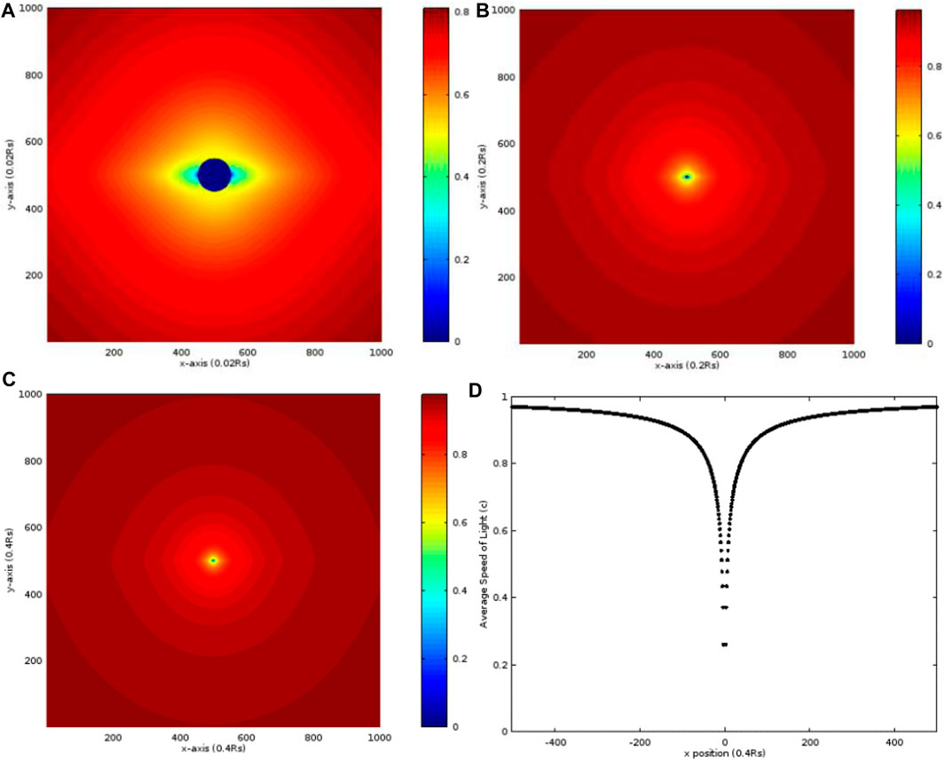
FIGURE 1. Distribution of the average radial speed of light in units of c, calculated from r = R_S to the random point S, in the case that a = 1.0 R_S and R_Q = 0.1 R_S. The maximums of x and y are both (A) 10 R_S, (B) 100 R_S, and (C) 200 R_S. (D) Distribution of the average radial speed of light along the x-axis in (C).

Then, we consider the case of a = 100 R_S and R_Q = 0.1 R_S. It is very explicit that the highest average radial speed of more than 20.0 c mainly distributes in a very narrow range near the x-axis as shown in Figure 2A, and the maximum is close to 45.0 c. The average radial speed quickly drops to about 10 c as r = 20 R_S as shown in Figures 2B and C. As r increases, it gradually goes to c. Comparing the calculations with those in Figure 1, the highest average speed is not on the y-axis. On the contrary, the highest value appears on the x-axis and the slowest one on the y-axis at the same r. Similar to Figure 1D, the distribution along the x-axis is shown in Figure 2D where the maximum of r is 200 R_S symmetrical to the center. In particular, the maximum on the x-axis is not at the place adjacent to R_S but a little away from R_S. The maximum is at about r = 2 R_S.

FIGURE 2

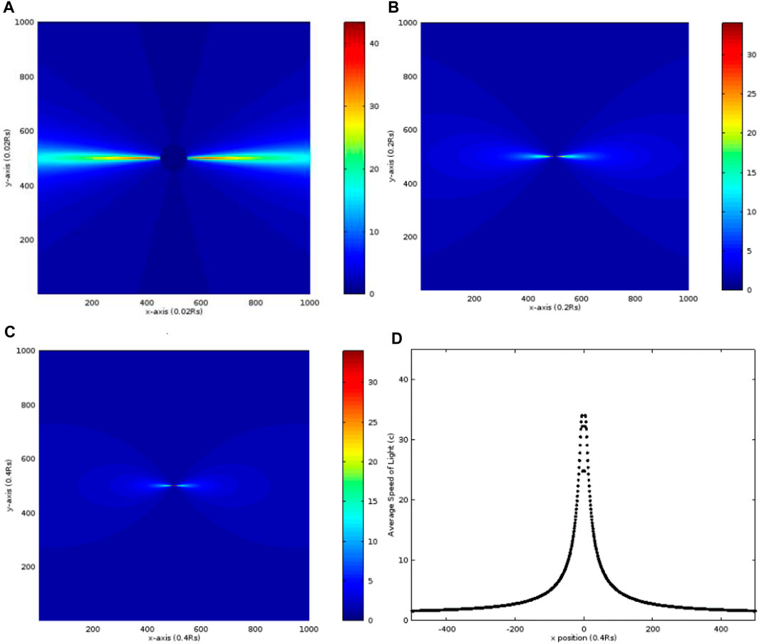
FIGURE 2. Distribution of the average radial speed of light in units of c, calculated from r = R_S to the random point S, in the case that a = 100 R_S and R_Q = 0.1 R_S. The maximums of x and y are both (A) 10 R_S, (B) 100 R_S, and (C) 200 R_S. (D) Distribution of the average radial speed of light along the x-axis in (C).

The third case is similar to the first one in which a = R_S but R_Q increases from 0.1 R_S to 1.0 R_S However, the results are much different from those in Figure 1. In Figure 3A, the maximum is at the place adjacent to R_S on the x-axis, and a lot of places show the average radial speed of more than 0.8 c. Therefore, increasing R_Q from 0.1 R_S to 1.0 R_S also raises the average radial speed and changes the distribution. In Figures 3B and C, the distributions in the larger ranges show that the variation along the x-axis is larger than that along the y-axis and the equi-speed surfaces are elliptic shapes. The distribution along the x-axis in Figure 3C is drawn in Figure 3D where the average radial speed is about 1.4 c adjacent to R_S and quickly drops to the minimum of roughly 0.85 c at about r = 4.0 R_S. The maximum of r is 200 R_S symmetrical to the center in Figure 3D. After this minimum, it slowly increases close to 1.0 c. Along each direction, all average radial speeds show similar trends reaching 1.0 c when r increases largely.

FIGURE 3

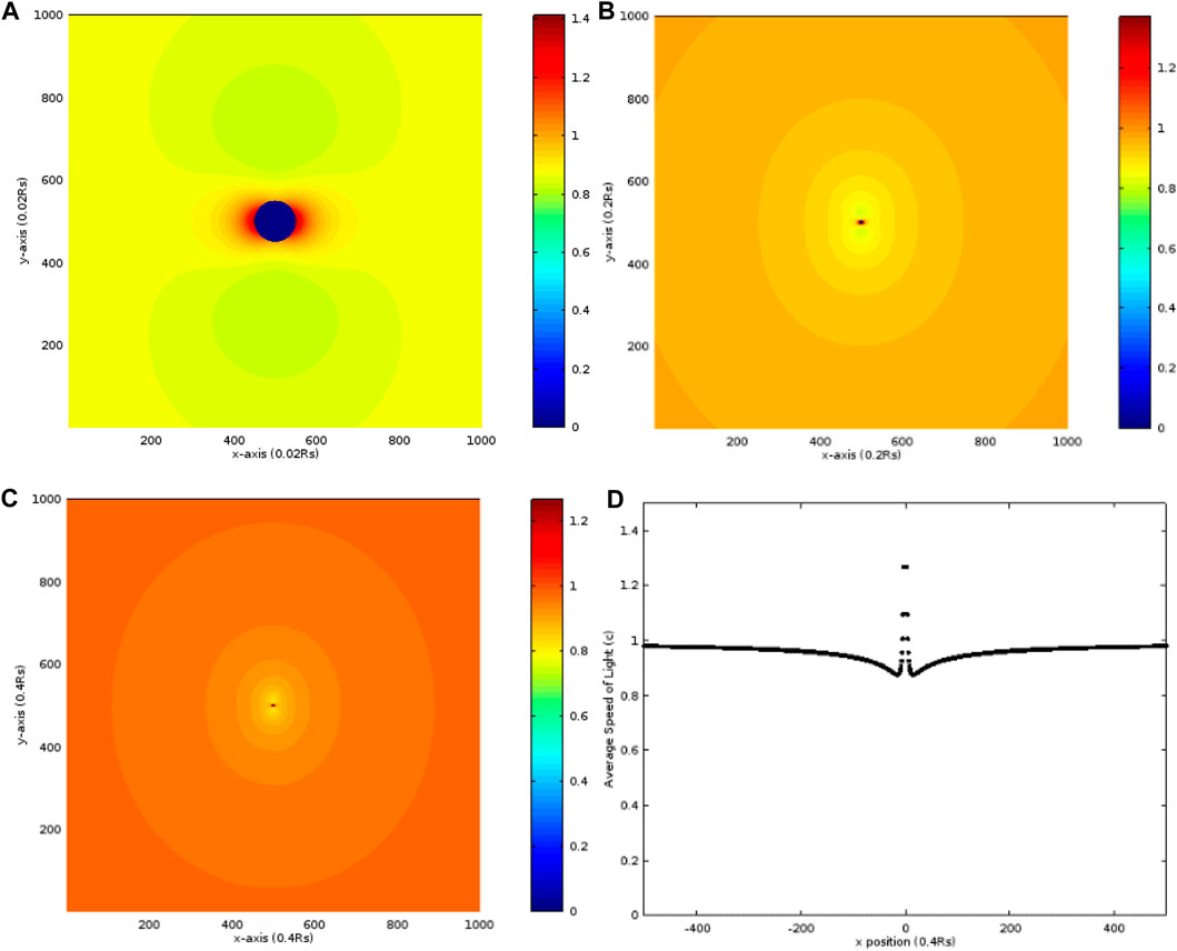
FIGURE 3. Distribution of the average radial speed in units of c, calculated from r = R_S to the random point S, in the case that a = 1.0 R_S and R_Q = 1.0 R_S. The maximums of x and y are both (A) 10 R_S, (B) 100 R_S, and (C) 200 R_S. (D) Distribution of the average radial speed of light along the x-axis in (C).

The fourth case holds R_Q equal to 1.0 R_S but increases a to 10.0 R_S. In Figure 4A, the maximum of about 10.0 c is also adjacent to R_S on the x-axis. The average radial speed of more than half maximum distributes in a narrow range near the x-axis but is not like the result in Figure 2 where the distribution is more centralized to the x-axis. As enlarging the calculation range, the average radial speed of more than 2.0 c mainly distributes near the x-axis and very close to R_S as shown in Figures 4B and C. The distribution of the average radial speed along the x-axis is drawn in Figure 4D, in which it drops very quickly from the place adjacent to R_S to 200 R_S. Finally, the average radial speed is close to 1.0 c as r is very large in our calculations.

FIGURE 4

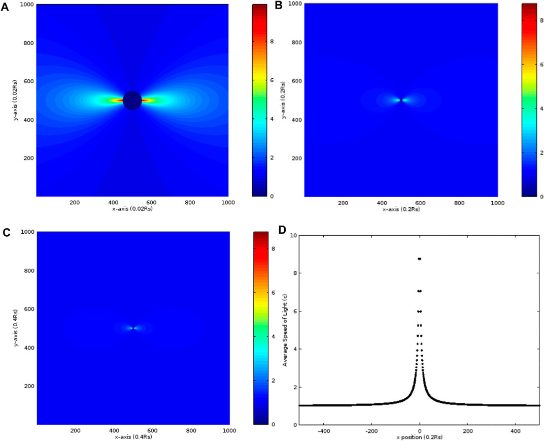
FIGURE 4. Distribution of average radial speed in units of c, calculated from r = R_S to the random point S, in the case that a = 10 R_S and R_Q = 1.0 R_S. The maximums of x and y are both (A) 10 R_S, (B) 100 R_S, and (C) 200 R_S. (D) The distribution of the average radial speed of light along the x-axis in (C).

The fifth case uses the same R_Q = 1.0 R_S and a is increased to 50 R_S in order to investigate the effect of the rotation on the average radial speed. In Figure 5A, the distribution of the average radial speed of more than 20.0 c is very close to the axis symmetric to the center within 4.0 R_S. The maximum of about 50.0 c is also adjacent to R_S on the x-axis. Comparing Figure 5A with Figure 4A, it shows this distribution closer to the x-axis and more centralized. In the enlarged space as shown in Figures 5B and C, the average radial speed of more than 20.0 c is close to the center. The distribution of the average radial speed along the x-axis is shown in Figure 5D where it quickly drops from the place adjacent to R_S to 200 R_S and the calculation is close to 1.0 c the same as in previous cases.

FIGURE 5

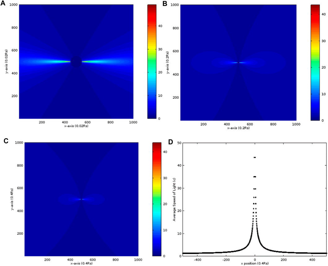
FIGURE 5. Distribution of the average radial speed of light in units of c, calculated from r = R_S to the random point S, in the case that a = 50 R_S and R_Q = 1.0 R_S. The maximums of x and y are both (A) 10 R_S, (B) 100 R_S, and (C) 200 R_S. (D) The distribution of the average radial speed of light along the x-axis in (C).

The sixth case continues the previous discussion where R_Q is still 1.0 R_S and a is increased to 100 R_S. In Figure 6A, the maximum of about 100.0 c is also adjacent to R_S on the x-axis. The distribution of the average radial speed of more than 40.0 c is much closer to the x-axis symmetric to the center and its range is within 4.0 R_S. When enlarging the calculation space, it shows the average radial speed of more than 40.0 c close to the center as shown in Figures 6B and C. The distribution along the x-axis is shown in Figure 6D where it quickly drops to 1.0 c from R_S to 200 R_S, and the calculation reveals the same result as the previous cases.

FIGURE 6

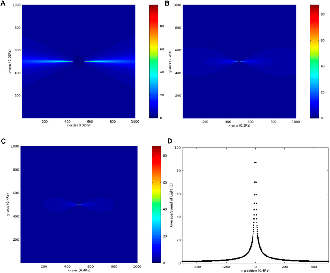
FIGURE 6. Distribution of the average radial speed of light in units of c, calculated from r = R_S to the random point S, in the case that a = 100 R_S and R_Q = 1.0 R_S. The maximums of x and y are both (A) 10 R_S, (B) 100 R_S, and (C) 200 R_S. (D) The distribution of the average radial speed of light along the x-axis in (C).

Then, we compare these cases with each other and find out the effects of R_Q and a. Each data is discrete and we connect them in a smooth curve. In Figure 7A, we investigate the effect of R_Q using the calculations in Figures 1D, 2D and Figures 3D, 6D. The figure shows log₁₀ of all curves. Comparing Figure 1D with Figure 3D, the case of 0.1 R_Q shows the minimum adjacent to R_S, and the case of 1.0 R_Q has a maximum adjacent to R_S and then drops to a minimum a little away from R_S. Both cases show very close values when r is more than 80 R_S and then gradually increase to zero when r = 200 R_S. For another two cases of 0.1 R_Q and 1.0 R_Q with the same a = 100 R_S, the smaller R_Q shows a drop when r is close to R_S and the maximum is at a distance a little away from R_S, whereas the bigger one has a maximum adjacent to Rs. Both values almost overlap when r is larger than 4.0 R_S and gradually decrease to zero as r increases largely. So the larger rotational term a needs longer distance to reach the average radial speed close to 1.0 c. The same result is also revealed in the four different rotation cases where R_Q holds at 1.0 R_S as shown in Figure 7B. All curves show the maximums adjacent to R_S and decrease to zero as r is large enough. It means when the observer is far away from the black hole, the measurement of the average radial speed of light is close to c as we measure on the Earth. This result can be applied to other superstars that produce strong gravity with high rotation.

FIGURE 7

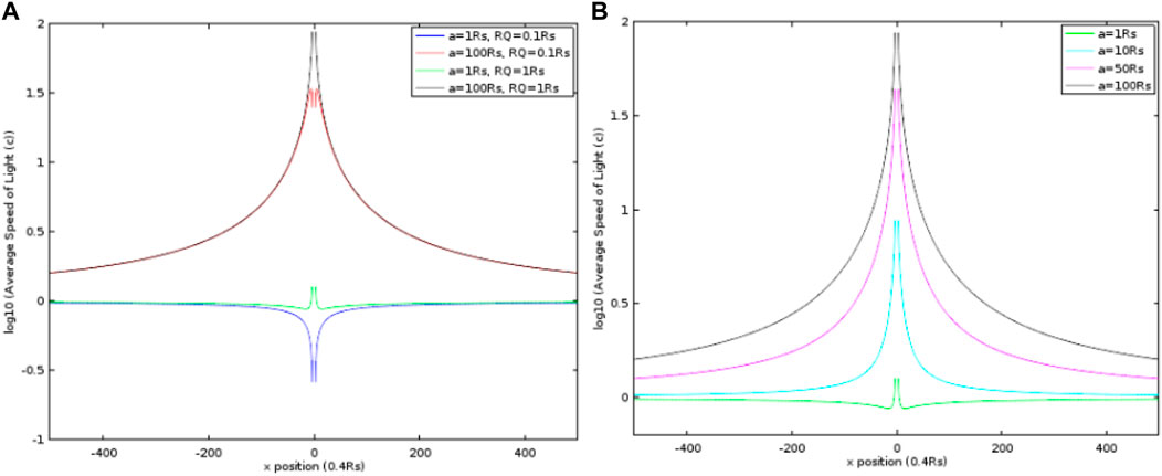
FIGURE 7. (A) Log₁₀ of the smooth curves from Figures 1D, 2D, 3D, 6D. (B) Log₁₀ of the smooth curves from Figures 3D–6D.

6 Why the Speed of the Massive Particle Is Astronomically Measured Faster Than That of Light?

According to the previous results, the average radial speed of light is possibly more than c very tiny from the black hole to a faraway place such as the Earth as long as the radial speed is the dominant part. Some reports (Blandford et al., 1977; Mirabel and Rodríguez, 1994; Rodríguez and Mirabel, 1995; Belloni et al., 1997; Orosz et al., 2001; Cheung et al., 2007; Asada et al., 2014a) showed that the speed of the particle away from the black hole was measured faster than c. This kind of phenomenon violates the special relativistic theory and makes us think about other possibilities. Here, we use our results to give another explanation.

As we know, there exists significant light bending near the superstar or black hole due to the strong gravity. Gravitational lensing is an example (Ehlers and Rindler, 1997). Then, we consider the relativistically electric particles leaving the black hole and radiating electromagnetic waves at two places A and B as shown in Figure 8. Supposing the time difference measured in the Earth system is 1 year and the speeds of the particles are all less than c. So how can the measurements on the Earth give particles faster than c? As shown in Figure 8, light radiated at place A forwards to the Earth and will be received after time t. Then, when the particles move to place B, light is radiated and will be received after time t-1 year on the Earth, the actual path for the particles is along AB and the actual length is AB. Light emitted at A is along the trajectory with the average speed c₁ and light emitted at B is along the other one with the average speed c₂. The time difference between these two trajectories is 1 year, and the former spending time is more than the latter. Due to the strong gravitation, two trajectories are curved near the black hole and approximate two straight lines far away from the black hole. The curvature of the light trajectory from A can be larger than that from B. Due to the light bending, the observed path of the particles is along A′’B′, not AB. We call the path A′B′ the imaging path and its distance the imaging length. The phenomenon is much similar to the observation of particles in water by an observer above water. The different refraction indices between water and air cause light to change its direction at the interface and result in the observer thinking of the particle is in shallow water. Therefore, the light bending near the black hole results in the imaging length A′B′ longer than the actual length AB. The ratio of A′B′ to AB might be several times, so it gives the results of the particles faster than c.

FIGURE 8

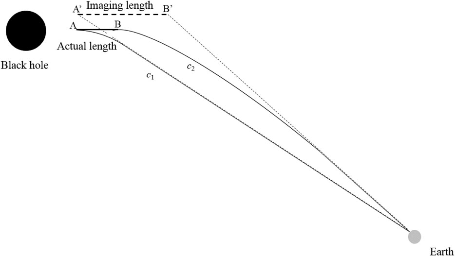
FIGURE 8. Two light trajectories with different average speeds cause the visual illusion in astronomical observations. It would result in the conclusion of the faster-than-light particle. Here, c₁ and c₂ are very close to c and possibly more or less than c being very tiny.

After all, special relativity (Marion and Thornton, 1988) tells us that the massive particle cannot be speeded higher than c and its relativistic mass is close to infinite when the speed is very close to c. This principle has been verified in each operation on the synchrotron accelerator, and it always needs a lot of energy to speed an electron close to c. We would expect that it is also the same phenomenon in most places even near the black hole because the massive particle is far away from the black hole with only finite total energy and its energy would be conserved even when it moves to the neighboring place of the black hole. However, when the speed of the massive particle is faster than the speed of light, it might be expected that a phenomenon like Cherenkov’s radiation would be observed in the regions near the black hole, some supermassive stars, or planets with strong gravity.

The speed of light near a massively rotating and charged black hole can be observed faster than it on Earth. This result can be one way to explain the flares near the black hole at IC 310 recorded on 12/13 November 2012 (Aleksić et al., 2014). The second way to explain the superluminal phenomena of the massive jets ejected from some quasars or black holes [−7] is based on our discussions. The superluminal phenomenon of light from the Earth’s viewpoint is the reason that we measure or observe the speed of light by the definition of dr/dt, not dr/dτ in the spontaneously local reference frame. Actually, the speed of light in the local reference frame near some quasars or black holes is still c, but it may be observed or measured to be larger than c on the Earth. According to the same statement, it is easy to speculate that the massive particles fully or most partly moving along the radial direction away from some quasars or black holes are possibly observed in their superluminal phenomena on the Earth, as long as their speeds in the spontaneously local reference frames are very close to c. Therefore, we can observe some relativistically massive jets moving faster than c near some quasars or black holes (Blandford et al., 1977; Mirabel and Rodríguez, 1994; Rodríguez and Mirabel, 1995; Belloni et al., 1997; Orosz et al., 2001; Cheung et al., 2007; Asada et al., 2014a).

7 Comparison With Other Theories Explaining the Superluminal Light

There are also some theories to explain the superluminal light in astronomy. In the following, two previous theories are reviewed. The first one is the corrections to the local propagation of photons calculated by the quantum electrodynamics (QED) contribution of the one-loop vacuum polarization to the photon effective action on a generally curved background manifold (Drummond and Hathrell, 1980). The so-called vacuum polarization is the photon being virtue e⁻-e⁺ pair for part of the time (Drummond and Hathrell, 1980; Shore, 1996; Cho, 1997). The two leading terms in the photon effective action are (Drummond and Hathrell, 1980; Daneils and Shore, 1994; Daneils and Shore, 1996; Shore, 1996; Cho, 1997; Cai, 1998; Shore, 2006; Hallowood and Shore, 2008; De Rham and Andrew, 2020)

$W=W_0+W_1=\int d^{4}x\sqrt{-g}\left[-\frac{1}{4}{F}_{\mu \nu }{F}^{\mu \nu }+\frac{1}{m_e^2}\left(aR{F}_{\mu \nu }{F}^{\mu \nu }+b{R}_{\mu \nu }{F}^{\mu \sigma }{F}_{\sigma }^v+c{R}_{\mu \nu \sigma \tau }{F}^{\mu \nu }{F}^{\sigma \tau }+d{D}_{\mu }{F}^{\mu \nu }{D}_{\sigma }{F}_v^{\sigma }\right)\right],(61)$

where the Minkowski metric $g^{\mu \nu }=diag\left(1,-1,-1,-1\right)$ (Drummond and Hathrell, 1980), the Riemann curvature tensor $R_{v\sigma \tau }^{\mu }={\Gamma }_{v\tau ,\sigma }^{\mu }-{\Gamma }_{v\sigma ,\tau }^{\mu }+{\Gamma }_{\lambda \sigma }^{\mu }{\Gamma }_{v\tau }^{\lambda }-{\Gamma }_{\lambda \tau }^{\mu }{\Gamma }_{v\sigma }^{\lambda }$ (Drummond and Hathrell, 1980), F^μν is the electromagnetic field strength, m_e is the electron mass (Drummond and Hathrell, 1980; Daneils and Shore, 1994; Daneils and Shore, 1996; Shore, 1996; Cho, 1997; Cai, 1998; Dogov and Novigov, 1998; Shore, 2006; Hallowood and Shore, 2008; De Rham and Andrew, 2020), a = -5α/720π (Drummond and Hathrell, 1980; Daneils and Shore, 1994; Daneils and Shore, 1996; Shore, 1996; Cho, 1997; Cai, 1998), b = 26α/720π (Drummond and Hathrell, 1980; Daneils and Shore, 1994; Daneils and Shore, 1996; Shore, 1996; Cho, 1997; Cai, 1998), c = -2α/720π (Drummond and Hathrell, 1980; Daneils and Shore, 1994; Daneils and Shore, 1996; Shore, 1996; Cho, 1997; Cai, 1998), and d = -24α/720π (Daneils and Shore, 1994; Daneils and Shore, 1996; Cho, 1997; Cai, 1998) in terms of the fine structure constant α. The coefficients a, b, and c reveal the influence of the curvature functional, and d may be obtained from the flat-space vacuum polarization amplitude which represents the mass-off-shell effect (Drummond and Hathrell, 1980). The next term in the photon effect action is (Daneils and Shore, 1994; Cho, 1997; Cai, 1998)

$W_2=\frac{1}{m_e^4}\int d^{4}x\sqrt{-g}\left[y{F}_{\mu \nu }{F}_{\sigma \tau }{F}^{\mu \sigma }{F}^{\nu \tau }+z{\left(F_{\mu \nu }{F}^{\mu \nu }\right)}^2\right],(62)$

where y = 56α²/720π and z = −20α²/720π (Daneils and Shore, 1994; Cho, 1997; Cai, 1998). This action is used to discuss the quantum correction of photon propagation near the Reissner–Nordström black hole of mass M and charge Q (Daneils and Shore, 1994), the topological black hole (Cai, 1998), and the dilaton black hole (Cho, 1997). The photon effective action in Eq. 61 leads to the gravitational modified equation of motion for the photon (Drummond and Hathrell, 1980; Daneils and Shore, 1994; Daneils and Shore, 1996; Cho, 1997; Cai, 1998)

$D_{\mu }{F}^{\mu \nu }+\frac{\delta W_1}{\delta A_{\mu }\left(x\right)}=0.(63)$

This equation shows D_μF^μν in order of O(e²) but the term involving the coefficient d influences the motion to O(e⁴) (Drummond and Hathrell, 1980). Usually, it can be omitted due to its very small influence. Therefore, the photon equation of motion approximates (Drummond and Hathrell, 1980; Daneils and Shore, 1994; Shore, 1996)

$D_{\mu }{F}^{\mu \nu }+\frac{1}{m_e^2}{D}_{\mu }\left[4aR{F}^{\mu \nu }+2b\left(R_{\sigma }^{\mu }{F}^{\sigma \nu }-R_{\sigma }^v{F}^{\sigma \mu }\right)+4c{R}_{\sigma \tau }^{\mu v}{F}^{\sigma \tau }\right]=0.(64)$

The more complicated photon equation of motion including the d and W₂ terms is (Daneils and Shore, 1994; Cho, 1997; Cai, 1998)

$\begin{array}{c}{D}_{\mu }{F}^{\mu \nu }+\frac{1}{m_e^2}[4a{D}_{\mu }\left(R{F}^{\mu \nu }\right)+2b{D}_{\mu }\left(R_{\sigma }^{\mu }{F}^{\sigma \nu }-R_{\sigma }^v{F}^{\sigma \mu }\right)\\ +4c{D}_{\mu }\left(R_{\sigma \tau }^{\mu v}{F}^{\sigma \tau }\right)+2d\left(D^2{D}_{\sigma }{F}^{\sigma \nu }-D_{\mu }{D}^{\nu }{D}_{\sigma }{F}^{\sigma \mu }\right)]\\ -\frac{1}{m_e^4}[8z\left(F^{\sigma \tau }{F}_{\sigma \tau }{D}_{\mu }{F}^{\mu \nu }+2F^{\mu \nu }{F}_{\sigma \tau }{D}_{\mu }{F}^{\sigma \tau }\right)\\ +8y\left(F^{\nu \tau }{F}_{\sigma \tau }{D}_{\mu }{F}^{\mu \sigma }+F^{\mu \sigma }{F}_{\sigma \tau }{D}_{\mu }{F}^{\nu \tau }+F^{\mu \sigma }{F}^{\nu \tau }{D}_{\mu }{F}^{\sigma \tau }\right)]=0.\end{array}(65)$

Without the one-loop quantum correction, we have D_μF^μν = 0 (Drummond and Hathrell, 1980; Shore, 1996; Cho, 1997; Cai, 1998). To study the photon equation of motion, the simplest way is to use the geometrical-optics plane-wave approximation in a gauge-invariant manner by setting F_μν = f_μνe^iθ, where f_μν is a slowly varying amplitude and θ is the rapidly varying phase with the photon momentum k_μ = D_μθ (Daneils and Shore, 1994; Daneils and Shore, 1996; Shore, 1996; Cho, 1997; Cai, 1998; Shore, 2006; Hallowood and Shore, 2008). The electromagnetic Bianchi identity becomes (Drummond and Hathrell, 1980; Daneils and Shore, 1994; Shore, 1996; Cai, 1998)

$k_{\rho }{f}_{\mu \nu }+k_{\mu }{f}_{\nu \rho }+k_{\nu }{f}_{\rho \mu }=0.(66)$

Furthermore, it gives $f_{\mu \nu }=k_{\mu }{a}_{\nu }-k_{\nu }{a}_{\mu }$ (Drummond and Hathrell, 1980; Daneils and Shore, 1994; Daneils and Shore, 1996; Shore, 1996; Cho, 1997; Cai, 1998; Dogov and Novigov, 1998; Shore, 2006) where a_μ is the polarization vector of the photon with the condition a^μa_μ = −1 (Daneils and Shore, 1994; Daneils and Shore, 1996; Shore, 1996; Cho, 1997; Cai, 1998; Dogov and Novigov, 1998; Shore, 2006). This polarization vector is orthogonal to the momentum that k^μa_μ = 0 (Drummond and Hathrell, 1980; Daneils and Shore, 1996; Cho, 1997). Then, we can obtain the light cone condition (Daneils and Shore, 1996; Shore, 1996; Shore, 2006)

$k^2-\frac{2b}{m_e^2}{R}_{\mu \lambda }{k}^{\mu }{k}^{\lambda }+\frac{8c}{m_e^2}{R}_{\mu \nu \lambda \rho }{k}^{\mu }{k}^{\lambda }{a}^{\nu }{a}^{\rho }=0.(67)$

The quantum corrections showed the tidal gravitational forces altering the low-energy speeds of photons greater than c in some cases (Drummond and Hathrell, 1980; Daneils and Shore, 1994; Daneils and Shore, 1996; Shore, 1996; Cho, 1997; Cai, 1998; Shore, 2006; Hallowood and Shore, 2008; De Rham and Andrew, 2020). The speed of light c used here is the value in vacuum without gravity. Initially, this non-dispersive and gauge-invariant effect was demonstrated on the Schwarzschild background in which the low-energy speed of the photon traveling transversely (with momentum in the angular direction) is found to be the form (Drummond and Hathrell, 1980)

$\left|\frac{k_t}{k_{\varnothing }}\right|\approx \left\{1+\frac{1}{2}\left[\frac{\frac{3R_s}{r^3}\left(\frac{\alpha }{90\pi m_e^2}\right)}{1+\frac{R_s}{r^3}\left(\frac{\alpha }{90\pi m_e^2}\right)}\right]\right\}\approx 1+\frac{\alpha }{60\pi m_e^2}\frac{R_S}{r^3}.(68)$

On the other hand, for the Reissner–Nordström black hole of mass M and charge Q, the unchanged radial photon velocity and two physically polarization-dependent orbital photon velocities are given (Daneils and Shore, 1994). The two orbital photon velocities are

${\left|\frac{k_t}{k_{\varnothing }}\right|}_{r-polarized}\approx 1+\frac{\alpha }{60\pi m_e^2}\frac{R_S}{r^3}+\frac{\alpha }{36\pi m_e^2}\frac{R_Q^2}{4\pi r^4}-\frac{{\alpha }^2}{45\pi m_e^4}\frac{R_Q^2}{4\pi r^4}(69)$

and

${\left|\frac{k_t}{k_{\varnothing }}\right|}_{\theta -polarized}\approx 1-\frac{\alpha }{60\pi m_e^2}\frac{R_S}{r^3}+\frac{13\alpha }{180\pi m_e^2}\frac{R_Q^2}{4\pi r^4}-\frac{7{\alpha }^2}{90\pi m_e^4}\frac{R_Q^2}{4\pi r^4}.(70)$

The first term in both equations is the gravitational contribution identical to the Schwarzschild background in Eq. 67. Whether it is superluminal or not is dependent on the relative magnitude of the quantum corrections in Eq. 68 (Daneils and Shore, 1994). Another spherically symmetric spacetime is the dilaton black hole (Cho, 1997), in which to first-order perturbation, the radially directed photons gives

$\left|\frac{k_t}{k_r}\right|\approx 1-\frac{1}{2m_e^2}\left(b+2c\right)\frac{{\widehat{a}}^2}{{\left(1+{\widehat{a}}^2\right)}^2}\left(\frac{r_{-}^2}{r^4}\right)\left(1-\frac{r_{+}}{r}\right){\left(1-\frac{r_{-}}{r}\right)}^{-1},(71)$

where

$\frac{2GM}{c^2}=r_{+}+\left(\frac{1-{\widehat{a}}^2}{1+{\widehat{a}}^2}\right)r_{-}(72)$

and

$\frac{KG{Q}^2}{c^4}=\frac{r_{+}{r}_{-}}{1+{\widehat{a}}^2}.(73)$

The light-cone condition is modified considering the QED quantum corrections. The radial photons in fact propagate superluminally when r > r₊, r_- in this dilatonic case even though the spacetime is still spherically symmetric. About the rotating black hole (Daneils and Shore, 1996), the radial motion for photons on the equatorial plane, the velocity shift is (Daneils and Shore, 1996)

$\Delta v=\left|\frac{k_t}{k_r}\right|-1=\pm \left(A+2B\right)ϵ=\mp ϵ\left(\frac{3M{a}^2{r}^3}{{\rho }^6{\mathrm{\Sigma }}^2}\Delta \right),(74)$

where

$\mathrm{\Sigma }={\left(r^2+a^2\right)}^2-a^2{\sin }^2\theta \mathrm{\Delta }.(75)$

It means the photon is possibly superluminal along the radial direction.

Furthermore, not only the correction speeds of photons but also the correction speeds of gravitational waves are proposed in the curved spacetime. Using a gravitational field effective theory (De Rham and Andrew, 2020),

$L=\sqrt{-g}\left[\frac{M_{pl}^2}{2}R-\frac{1}{2}{\left(\partial \varphi \right)}^2+\frac{a}{4M^4}{\left(\partial \varphi \right)}^4\right],(76)$

and considering a modification to the low-energy speed, it gives c_s different from unity:

$c_s^2=1+\frac{\left|a\right|{\dot{\varphi }}^2}{M_{pl}^2{M}^2}+\dots .,(77)$

where $\varphi$ is the amplitude of the propagating wave.

To sum up, the vacuum polarization in QED is thought to cause the superluminal low-frequency phase velocity of photons propagating in a non-dynamically curved spacetime (Daneils and Shore, 1996; Hallowood and Shore, 2008). All superluminal phenomena discussed in references 1–10 exist in the local Lorentz coordinate system. Some people even mentioned that the tidal effect seems to strangely change the causal structure of the manifold (Drummond and Hathrell, 1980). Due to the quantum correction of photons in curved spacetime, it even gives a surprising result that in some reference frames, based on the possibility of closed time-like trajectories, photons can return to their source before they are produced (Dogov and Novigov, 1998). However, the spacelike photon momentum given by the light-cone condition inevitably involves the problem of causal paradox (Daneils and Shore, 1994). This is the most serious problem we must face. Therefore, the author proposes that either a time machine is possible in principle, or the superluminal propagation of photons due to the quantum correction of the one-loop vacuum polarization is problematic (Dogov and Novigov, 1998).

Another key question is whether this superluminal propagation can be observed in principle (Daneils and Shore, 1994). In other words, we have to face the other serious question, that is, does the vacuum polarization in curved spacetime always occur, or does it randomly exist at a certain time? When we calculate the quantum correction in curved spacetime, it clearly points out that the one-loop vacuum polarization in QED is an effect in which a photon is converted into a virtual e⁻-e⁺ pair for part of the time (Drummond and Hathrell, 1980; Cho, 1997; Cai, 1998). In fact, the randomness of such virtual e⁻-e⁺ pairs causes the phenomenon of the superluminal of light to occur randomly. Therefore, the superluminal light based on the quantum correction caused by the vacuum polarization in the curved spacetime becomes unexpected, and it cannot be observed always. This is the second question we must ask can we really observe this kind of superluminal phenomenon or gravitational birefringence? Especially, this phenomenon of the superluminal light caused by the one-loop vacuum polarization can have more possibility to take place near the super-gravitation source. Therefore, the physical significance of our contribution and study lies in deriving the superluminal phenomenon of light observed in a reference frame far away from a super-gravitational source such as on the Earth, which is different from the above discussion in the local Lorentz frame.

The other theory reported in 1966 (Rees, 1966) was proposed to explain the superluminal observations (Blandford et al., 1977; Pearson et al., 1981; Schilizzi and de Bruyn, 1983; Davis et al., 1985; Mirabel and Rodríguez, 1994; Rodríguez and Mirabel, 1995; Belloni et al., 1997; Abraham and Romero, 1999; Briretta et al., 1999; Junor et al., 1999; Orosz et al., 2001; Qian et al., 2001; Cheung et al., 2007; Asada et al., 2014a; Asada et al., 2014b; Snios et al., 2019) in astronomy due to the optical illusion caused by the object partly moving in the direction of the observer. In this theory, the Doppler factor δ is (Davis et al., 1985; Mirabel and Rodríguez, 1994; Briretta et al., 1999; Qian et al., 2001)

$\delta =\frac{1}{\gamma \left(1-\beta \cos \theta \right)},(78)$

and the apparent velocity v_c is (Blandford et al., 1977; Pearson et al., 1981; Davis et al., 1985; Briretta et al., 1999; Qian et al., 2001)

$v_c=\frac{c\beta \sin \theta }{\left(1-\beta \cos \theta \right)},(79)$

where v₀ = cβ is the space speed of the moving body, θ is the angle between the velocity of the moving body and the line of sight of the observer, and the Lorentz factor $\gamma ={\left(1-{\beta }^2\right)}^{-1}$. However, this is a problematic expression and easy to check that v_c→0 at θ→0. It is a wrong result because it tells us that we never see any body approaching us along the line of sight of the observer. Moreover, the theory mentioned earlier has been applied for the measurement of the moving body through the sound wave on the Earth. Therefore, it may predict to detect many faster-than-sound phenomena easily when the bodies move partly toward the observer according to this theory. Even if the moving body is slower than the sonic wave, the theory still predicts a possibly faster-than-sound phenomenon on the Earth. The Doppler effect used to explain the observed change of the light wavelength in special relativity (Klinaku, 2016) is demonstrated in Figure 9. The theory proposed in the references (Rees, 1966; Rees, 1967) belongs to the field of special relativity. Whether the Doppler effect can explain the superluminal motion or only the change of the light wavelength is worth further discussion. In special relativity, the speed of light is a constant no matter which reference frame proceeds the velocity measurement. Thus, we would rather think about the Doppler effect changing the frequency or wavelength, not changing the speed of sound or light. However, this theory (Rees, 1966; Rees, 1967) does not disagree with our results here. On the contrary, we worry that this theory (Rees, 1966; Rees, 1967) only discussed the observed phenomenon in the flat spacetime, not the spacetime near the super-gravitational source like the black hole.

FIGURE 9

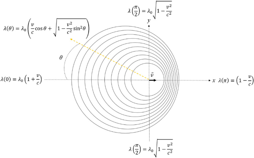
FIGURE 9. Doppler effect applied to the electromagnetic wave causing the change of wavelength in special relativity (Klinaku, 2016). This is a redrawn figure according to special relativity, and each circle represents the wave front. The wavelength of the light wave at the rest frame is λ₀ and the emitter moves at speed of v along the x-direction. The measured light wavelength λ(θ) is different at different observed angles θ due to the Doppler effect similar to the sound wave. In this figure, three observed wavelengths at 0, π/2, and π are also denoted by considering the relativistic effect.

As we know, many astronomically superluminal phenomena were reported near some very massive sources (Blandford et al., 1977; Pearson et al., 1981; Schilizzi and de Bruyn, 1983; Davis et al., 1985; Mirabel and Rodríguez, 1994; Rodríguez and Mirabel, 1995; Belloni et al., 1997; Abraham and Romero, 1999; Briretta et al., 1999; Junor et al., 1999; Orosz et al., 2001; Qian et al., 2001; Cheung et al., 2007; Asada et al., 2014a; Asada et al., 2014b; Snios et al., 2019), and the observation near the M87 black hole is a representation (Snios et al., 2019). Fortunately, the radio jet from the central black hole in M87 is not toward the observer on the Earth. Otherwise, we will be impacted by this relativistic jet resulting in a serious affection on the Earth’s living. After rigorous derivations, our results also show the main part of light along the radial direction can be observed faster than light. This phenomenon is from near to far space surrounding the central rotating and charged super-gravitational source. As long as the moving particles are very close to c in the local frame, then these particles can be observed faster than light in the far-distance frame on the Earth. Then, in the following, the M87 jet is used as an example to demonstrate our model.

The research about the M87 jet can be traced back 70 years. In the 1950s, it was discovered that the optical radiation emitted by the jet in M87 is synchrotron radiation performing strong polarization (Baade, 1956; Burbidge, 1956). Then, the phenomenon that the jet, from high-speed rotational Galaxy M87 (Stewart, 1971; Sparks et al., 1992; Briretta et al., 1999; Kovalev et al., 2007; Doeleman et al., 2012), radiates the polarized electromagnetic waves (Felten, 1968; Felten et al., 1970; Schmidt et al., 1978; Sparks et al., 1992; Cheung et al., 2007; Klein, 2007; Kovalev et al., 2007; Doeleman et al., 2012) can be explained by the accelerated electrons in an axial magnetic field. Researchers found that the M87 jet precesses and forms a spiral within a small conical angle because of the magnetic field from the nucleus of the black hole (Sparks et al., 1992; Kovalev et al., 2007). The plane-polarized light emitted by this jet suggested that light energy is produced by accelerated electrons moving in a magnetic field at relativistic velocities. At the same time, these accelerated electrons perform helical trajectories with a gradually increasing rotational radius along the axis (Persson, 1963). This jet was observed to extend five thousand light-years at least as shown in Figure 10 (Felten et al., 1970; Kovalev et al., 2007), and open a small polar angle of 6–7° at a distance of 37.5 light-years (12 pc) from the source (Kovalev et al., 2007).

FIGURE 10

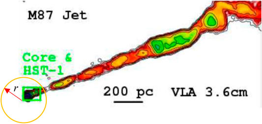
FIGURE 10. Multi-scale images of the M87 jet are shown in Reference (Cheung et al., 2007). It is a well-known M87 jet, extending at least 5,000 light-years. Here, we mainly use these images to demonstrate our model. When we discuss gravity and classical electrodynamics, the total mass as well as total charges have to be considered, respectively. This concept is also necessarily used in Einstein’s gravity when we use the Kerr–Newman metric. Theoretically speaking, if the observed point is on the sphere with radius r denoted by the yellow circle, the mass and charges within the sphere are necessarily considered to calculate the average radial speed of light in the Kerr–Newman metric. Therefore, not only the charges inside the black hole but also the charges surrounding the black hole are used. For simplicity, we suppose most parts of the effective charges distributing much wider than the Schwarzschild radius, about within several ten pc, used in the Kerr–Newman metric. The fixed approximate net charges are used to calculate points larger than several pc to several kpc in the M87 jet.

The fast electrons in this jet have been estimated to be ∼6 × 10⁵⁶ erg in the magnetic field B ∼ 6 × 10⁻⁶ G where the electromagnetic radiation above 10⁸ Hz is considered (Felten, 1968). The other estimation (Klein, 2007) reveals the total energy output of these electrons to be 5.1 × 10⁵⁶ erg (or 5.1 × 10⁴⁹ J or 3.2 × 10⁶⁸ eV). By comparison, the entire Milky Way only produces an estimated energy of about 5 × 10³⁶ J per second. Therefore, its energy is at least 10¹³ times as large as the emitted energy per second from the entire Milky Way. It means that this jet includes a lot of electrons, and the number of electrons can be estimated. If each electron on average possesses an energy of 10 MeV, then there are at least 5.1 × 10⁴² C electrons in this jet. In this average case, the Lorentz factor γ ∼ 20, so the correspondingly average speed of an electron is about 0.99875 c. If the average energy of an electron increases to 1 GeV, then there are at least 5.1 × 10⁴⁰ C electrons in this jet. Even though the average energy of electrons can be as high as 1 TeV (Stawarz et al., 2006; Cheung et al., 2007), at least 5.1 × 10³⁷ C electrons exist in this jet. Generally speaking, the average energy of 1 GeV would be a reasonable value for electrons in this jet. As we know, the lightest nucleus ¹H is 1,836 times heavier than one electron. According to this, we can speculate that most positively-charged nuclei or particles move much slower than the high-speed electrons, so these nuclei or particles exist much closer to the black hole, and the negatively-charged electrons move far away from the black hole at much faster speeds close to c (Felten et al., 1970). On the other hand, from the estimation of the blobs of hydrogen gas escaping the nucleus of the black hole (Felten et al., 1970), the mass speed of these blobs is v ∼ 0.06 c or more. This observation really reveals that the hydrogen gas moves much slower than electrons as expected. Therefore, the ejection of electrons in the M87 jet means a lot of positive charges far behind the relativistic electrons. If the energy of an electron were obtained initially the same as a charged particle like a proton or a hydrogen nucleus traveling at the above escaping speed, then the energy of an electron is about 1 GeV. Based on this fact, it is reasonable to assume the total charges surrounding the M87 black hole within several ten pc to be 10⁵∼10⁶ q where one q = 2.41 × 10³⁰ C. This charge q corresponds to $R_Q^2=KG{q}^2/c^4=R_S^2$ where K is the Coulomb’s constant and G is the Newton’s gravitational constant. The mass of the M87 black hole is about (6.2 ± 0.4) x 10⁹ M_ʘ (Doeleman et al., 2012), resulting in the maximum Schwarzschild radius of about 0.75 light-day. Then, Figure 1 in the reference (Stawarz et al., 2006) is used to demonstrate our model as shown in Figure 10. The concept of this model considers the total charges used in the Kerr–Newman metric, not only from those in the black hole but also from the charges surrounding the black hole because the fast-moving electrons leave many positive charges behind them, after the production of positive and negative charges in the sources. Although the tide charge parameter is introduced to study the extra hidden dimensions in the black hole spacetime (Banerjee et al., 2020; Banerjee et al., 2021; Mishra et al., 2021), we still use the real charge concept to easily and reasonably explain the observed superluminal phenomena (Blandford et al., 1977; Pearson et al., 1981; Schilizzi and de Bruyn, 1983; Mirabel and Rodríguez, 1994; Rodríguez and Mirabel, 1995; Belloni et al., 1997; Abraham and Romero, 1999; Briretta et al., 1999; Junor et al., 1999; Orosz et al., 2001; Qian et al., 2001; Cheung et al., 2007; Asada et al., 2014a; Asada et al., 2014b; Snios et al., 2019). When the observed point leaves the black hole further and further, more and more mass and charges from the black hole to the observed point can affect spacetime. Theoretically speaking, if the observed point is on the sphere with radius r, the mass and charges within the sphere are necessarily considered to calculate the average radial speed of light in the Kerr–Newman metric. Therefore, not only the charges inside the black hole are used but also the charges surrounding the black hole. Although most of the mass is gathered in the black hole, however, the distribution of charges extends a relatively long distance. However, the net charges shall decrease gradually and quickly from near to far space surrounding the black hole and most of them would mainly exist within several ten pc from the center of the black hole. In our discussions, for simplicity, we use constant net charges within several ten pc to calculate the average radial speed of light from several ten pc to 1,550 pc as shown in Figure 11A, where the constant net charges are 455,000 q, corresponding to R_Q = 455,000 R_S. Herein, we adopt each calculation point representing the average radial speed of light within one pc. Three calculation data are also denoted in Figure 11A. When the calculations are averaged by 1 year, three data vary between 1 and 4% only. We find that the calculated distribution of the average radial speed much matches the approximate fitting curve to the real observations in 2019 (Snios et al., 2019), as shown in Figure 11B. This approximate fitting curve is drawn to pass through the centers of the two data nearest the black hole. Furthermore, we can also present calculations close to the approximate fittings for the other observed data in different years by choosing different net charges in the Kerr–Newman metric. In addition, if the net charges are all consisting of the hydrogen nuclei, then the total mass of 455,000 q hydrogen nuclei equals 0.0057 M_ʘ or 8.66 × 10⁻¹³ times the M87 black hole. The mass corresponding to these hydrogen nuclei is much smaller compared to the M87 black hole thus they easily exist surrounding the black hole within several ten pc. So, our computations can be one explanation for the M87 jet ejected from the rotational black hole. Our model and calculations, based on the rotating and charged solution in general relativity, can give a reasonable explanation of the superluminal phenomena observed on the Earth.

FIGURE 11

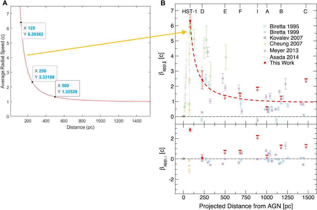
FIGURE 11. (A) Average radial speed of light along one radius from several ten pc to 1,550 pc in the equator plane calculated based on Eq. 30 where a = 0.10 R_S and R_Q = 455,000 R_S. Each data represent the average speed within one pc. Three calculation data are denoted in the figure. When the calculations are averaged by 1 year, these three data vary between 1 and 4% only. (B) Several observation reports of the radio jet from the central black hole in M87 from 1995 to 2019 (Snios et al., 2019). Although the average speeds of light are not coincident with each other, all the trends show the decreasing average radial speeds of light after a certain distance from the central black hole. The red dashed curve is the approximate fitting curve to the 2019 report without including the data near 1,500 pc. This fitting curve is much similar to the calculation curve in (A). It reveals that our model based on Eq. 30 is an explanation for the tangible observation about the M87 jet.

8 Conclusion

We use the Kerr–Newman metric based on general relativity to discuss the average radial speed of light from near to far space surrounding the black hole. First, according to the equivalence principle, time dilation requires some conditions between R_S, a, and R_Q. The geodesic of light is determined by ds² = 0 then we obtain the velocity equation of light described on the reference frame far away from the black hole like on the Earth. Next, we can calculate the spending time for light traveling from r = ${\alpha }_1{R}_S$ to r = ${\alpha }_2{R}_S$ along the radial direction at any $\theta$. We find that the average speed of light along the radial direction is possibly larger than c dependent on a and R_Q. Usually, the larger the a is, the higher the average radial speed of light is. The larger R_Q also benefits from a higher average radial speed. Higher rotation or larger charge of the black hole gives a longer range where the average radial speed is more than c, and it needs a longer distance to decrease and approach c. When an observer is far away from the black hole or other strong gravity, the measured average speed of light is close to c, as the measurement on the Earth. Based on these results, our explanation is also applicable to the observation of the faster-than-light massive particles like the M87 jet in astronomy.

In addition, two superluminal theories used to explain the speed of light in astronomy are compared. One is the Doppler effect in special relativity proposed 50 years ago, and the other is the change in the photon speed due to the QED contribution of one-loop vacuum polarization to the photon effective action in the general curved background manifold. The former seems to mainly appear as the change of the observed wavelength or frequency, while the latter is the possibly random and irregular occurrences. The Doppler effect has been applied on the observed wavelength of the sound wave dependent on the observed angle and the emitter velocity in air so the Doppler effect for the light wave in special relativity shall not be explained as the speed change of light in special relativity. On the other hand, although the QED contribution of one-loop vacuum polarization might predict the speed change of light, it probably only takes place for part of the time, that is, randomly occurs in spacetime, not always. Our explanation is based on the Kerr–Newman metric in general relativity, and it extends the discussion from the flat spacetime in special relativity to the curved spacetime which is suitable for many superluminal observations from near to far space surrounding the super-gravitational sources like the black hole.

Finally, we use the M87 jet as a tangible observation to be verified and explained by our calculations. The way we used to calculate the measured time on the Earth is based on Eq. 30 or Eq. 36. Then we use Eq. 59 to calculate the average radial speed of light traveling a distance. It tells us that the smaller the measured time is, the larger the average radial speed of light is. Because the fast-moving electrons leave many positive charges behind them after the production of positive and negative charges in the sources, the net charges are used to calculate the average radial speed of light in the Kerr–Newman metric, not only inside the black hole but also the charges surrounding the black hole. A demonstration is to consider the total charges surrounding the M87 black hole within several ten pc to be 455,000 q where one q = 2.41 × 10³⁰ C. The calculated distribution of the average radial speed of light from several ten pc to 1,550 pc as shown in Figure 11 much matches the approximate fitting curve to the real observations in 2019 (Snios et al., 2019). In summary, our model and calculations are used to explain the well-known superluminal phenomena in the M87 jet.

Data Availability Statement

The raw data supporting the conclusion of this article will be made available by the authors, without undue reservation.

Author Contributions

The single author proposed the research concept and derived all mathematical expressions. After building the mathematical form for the average radial speed of light near the Kerr–Newman gravitational source, he wrote all the programs to simulate and calculated the radial speed of light from the Kerr–Newman gravitational source like a rotating and charged black hole. Finally, he carefully obtained the whole results in this manuscript. He also read many references, completed this manuscript, and submitted this manuscript.

Conflict of Interest

The author declares that the research was conducted in the absence of any commercial or financial relationships that could be construed as a potential conflict of interest.

Publisher’s Note

All claims expressed in this article are solely those of the authors and do not necessarily represent those of their affiliated organizations, or those of the publisher, the editors, and the reviewers. Any product that may be evaluated in this article, or claim that may be made by its manufacturer, is not guaranteed or endorsed by the publisher.

Acknowledgments

The author thanks the Institute of Astronomy and Astrophysics at Academia Sinica in Taiwan for their encouragement. The author is also grateful to the reviewers for their comments to strengthen the statements in this article.

References

Abraham, Z., and Romero, G. E. (1999). Beaming and Precession in the Inner Jet of 3C 273. Astro. Astrophys. 344, 61–67.

Google Scholar

Adamo, T., and Newman, E. T. (2016). The Kerr-Newman Metric: A Review. arXiv: 1410.6626.

Google Scholar

Aleksić, J., Ansold, S., Antoneil, L. A., Babic, A., Barrio, J. A., Wilms, J., et al. (2014). Black Hole Lightning Due to Particle Acceleration at Subhorizon Scales. Sci 346, 1080. doi:10.1126/science.1256183

CrossRef Full Text | Google Scholar

Asada, K., Nakamura, M., Doi, A., Nagai, H., and Inoue, M. (2014). Discovery of SUB- TO SUPERLUMINAL MOTIONS IN THE M87 JET: AN IMPLICATION OF ACCELERATION FROM SUB-RELATIVISTIC TO RELATIVISTIC SPEEDS. Astrophys. J. Lett. 781, L2. doi:10.1088/2041-8205

CrossRef Full Text | Google Scholar

Asada, K., Nakamura, N., Doi, A., Nagai, H., and Inoue, M. (2014). Discovery of Sub- to Superluminal Motions in the M87 Jet: An Omplication of Acceleration from Sub-relativistic to Relativistic Speeds. Astrophys. J. Lett. 781, L2. doi:10.48550/arXiv.1311.5709

CrossRef Full Text | Google Scholar

Baade, W. (1956). Polarization in the Jet of Messier 87. ApJ 123, 550–551. doi:10.1086/146194

CrossRef Full Text | Google Scholar

Banerjee, I., Chakraborty, S., and SenGupta, S. (2021). Looking for Extra Dimensions in the Observed Quasi-Periodic Oscillations of Black Holes. J. Cosmol. Astropart. Phys. 9, 37. doi:10.1088/1475-7516/2021/09/037

CrossRef Full Text | Google Scholar

Banerjee, I., Chakraborty, S., and SenGupta, S. (2020). Sihouette of M87*: A New Window to Peek into the World of Hidden Dimensions. Phys. Rev. D. 101, 041301(R). doi:10.1103/physrevd.101.041301

CrossRef Full Text | Google Scholar

Belloni, T., Méndez, M., King, A. R., Van Der Klis, M., and Van Paradijs, J. (1997). An Unstable Central Disk in the Superluminal Black Hole X-Ray Binary GRS 1915+105. Astrophys. J. 479, L145–L148. doi:10.1086/310595

CrossRef Full Text | Google Scholar

Biggs, A. D., Browne, I. W. A., Helbig, P., Koopmans, L. V. E., Wilkinson, P. N., and Perley, R. A. (1999). Time Delay for the Gravitational Lens System B0218+357. Mon. Notices R. Astronomical Soc. 304, 349–358. doi:10.1046/j.1365-8711.1999.02309.x

CrossRef Full Text | Google Scholar

Blandford, R. D., Mckee, C. F., and Rees, M. J. (1977). Super-luminal Expansion in Extragalactic Radio Sources. Nature 267, 211–216. doi:10.1038/267211a0

PubMed Abstract | CrossRef Full Text | Google Scholar

Briretta, J. A., Sparks, W. B., and Macchetto, F. (1999). HUBBLE Space Telescope Observations of Superluminal Motion in the M87 Jet. Astrophys. J. 520, 621–626.

Google Scholar

Burbidge, G. R. (1956). On Synchrotron Radiation from Messier 87. ApJ 124, 416–429. doi:10.1086/146237

CrossRef Full Text | Google Scholar

Cai, R.-G. (1998). Propagation of Vacuum Polarized Photons in Topological Black Hole Spacetimes. Nucl. Phys. B 524, 639–657. doi:10.1016/s0550-3213(98)00274-0

CrossRef Full Text | Google Scholar

Cheung, C. C., Harris, D. E., and Stawarz, Ł. (2007). Superluminal Radio Features in the M87 Jet and the Site of Flaring TeV Gamma-Ray Emission. ApJ 663, L65–L68. doi:10.1086/520510

CrossRef Full Text | Google Scholar

Cho, H. T. (1997). "Faster Than Light" Photons in Dilaton Black Hole Spacetimes. Phys. Rev. D. 56, 6416–6424. doi:10.1103/physrevd.56.6416

CrossRef Full Text | Google Scholar

Daneils, R. D., and Shore, G. M. (1994). Faster Than Light Photons and Charged Black Holes. Nucl. Phys. 425, 634–650.

Google Scholar

Daneils, R. D., and Shore, G. M. (1996). Faster Than Light Photons and Rotating Black Holes. Phys. Lett. B 367, 75–83.

Google Scholar

Davis, R. J., Muxlow, T. W. B., and Conway, R. G. (1985). Radio Emission from the Jet and Lobe of 3C273. Nature 318, 343–345. doi:10.1038/318343a0

CrossRef Full Text | Google Scholar

De Felice, F., and Clarke, C. J. S. (1990). Relativity on Curved Manifolds. Cambridge: Cambridge University Press, 355 &362.

Google Scholar

De Rham, C., and Andrew, J. (2020). Tolley, “Causality in Curved Spacetimes: The Speed of Light and Gravity. Phys. Rev. D. 102, 084048. doi:10.1103/physrevd.102.084048

CrossRef Full Text | Google Scholar

Demorest, P. B., Pennucci, T., Ransom, S. M., Roberts, M. S. E., and Hessels, J. W. T. (2010). A Two-Solar-Mass Neutron Star Measured Using Shapiro Delay. Nature 467, 1081–1083. doi:10.1038/nature09466

PubMed Abstract | CrossRef Full Text | Google Scholar

Doeleman, S. S., Fish, V. L., Schenck, D. E., Beaudoin, C., Blundell, R., Bower, G. C., et al. (2012). Jet-Launching Structure Resolved Near the Supermassive Black Hole in M87. Science 338, 355–358. doi:10.1126/science.1224768

PubMed Abstract | CrossRef Full Text | Google Scholar

Dogov, A. D., and Novigov, I. D. (1998). Superluminal Propagation of Light in Gravitational Field and Non-causality Signals. Phys. Lett. B 442, 82–89.

Google Scholar

Drummond, I. T., and Hathrell, S. J. (1980). QED Vacuum Polarization in A Background Gravitational Field and its Effect on the Velocity of Photons. Phys. Rev. D. 22, 343–355. doi:10.1103/physrevd.22.343

CrossRef Full Text | Google Scholar

Ehlers, J., and Rindler, W. (1997). Local and Global Light Bending in Einstein's and Other Gravitational Theories. General Relativ. Gravit. 29, 519–529. doi:10.1023/a:1018843001842

CrossRef Full Text | Google Scholar

Felten, J. E., Arp, H. C., and Lynds, C. R. (1970). The M87 Jet. II. Temperature, Ionization, and X-Radiation in a Secondary-Production Model. ApJ 159, 415–425. doi:10.1086/150319

CrossRef Full Text | Google Scholar

Felten, J. E. (1968). The Radiation and Physical Properties of the M87 Jet. ApJ 151, 861–879. doi:10.1086/149488

CrossRef Full Text | Google Scholar

Gradshteyn, I. S., and Ryzhik, I. M. (2007). Table of Integrals, Series, and Products. 7th Ed. Burlington: Academic Press, 254.

Google Scholar

Hallowood, T. J., and Shore, G. M. (2008). The Refractive Index of Curved Spacetime: The Fate of Causality in QED. Nucl. Phys. B 795, 138–171. doi:10.48550/arXiv.0707.2303

CrossRef Full Text | Google Scholar

Hans, C. (1994). Ohanian and Remo Ruffini, Gravitation And Spacetime. 2nd ed. New York: W. W. Norton & Company&, 445460466492.

Google Scholar

Junor, W., Biretta, J. A., and Livio, M. (1999). Formation of the Radio Jet in M87 at 100 Schwarzschild Radii from the Central Black Hole. Nature 401, 891–892. doi:10.1038/44780

CrossRef Full Text | Google Scholar

Klein, U. (2007). The Large-Scale Structure of Virgo A. Radio Galaxy Messier 87, 55. doi:10.1007/BFb0106418

CrossRef Full Text | Google Scholar

Klinaku, S. (2016). The Doppler Effect and the Three Most Famous Experiments for Special Relativity. Results Phys. 6, 235–237. doi:10.1016/j.rinp.2016.04.011

CrossRef Full Text | Google Scholar

Kovalev, Y. Y., Lister, M. L., Homan, D. C., and Kellermann, K. I. (2007). The Inner Jet of the Radio Galaxy [OBJECTNAME STATUS="LINKS"]M87[/OBJECTNAME]. ApJ 668, L27–L30. doi:10.1086/522603

CrossRef Full Text | Google Scholar

Landau, L. D., and Lifshitz, E. M. (1975). The Classical Theory of Fields. Pergamon Press LTD., Fourth Revised English Edition, 309.

Google Scholar

Lovell, J. E. J., Jauncey, D. L., Reynolds, J. E., Wieringa, M. H., King, E. A., Tzioumis, A. K., et al. (1998). The Time Delay in the Gravitational Lens PKS 1830−211. Astrophys. J. 508, L51–L54. doi:10.1086/311723

CrossRef Full Text | Google Scholar

Marion, J. B., and Thornton, S. T. (1988). Classical Dynamics of Particles & Systems. 3rd ed. Orlando: Harcourt Brace Jovanovich, 507.

Google Scholar

Mirabel, I. F., and Rodríguez, L. F. (1994). A Superluminal Source in the Galaxy. Nature 371, 46–48. doi:10.1038/371046a0

CrossRef Full Text | Google Scholar

Mishra, A. K., Ghosh, A., and Chakraborty, S. (2021). Constraining Extra Dimensions Using Observations of Black Hole Quasi-Normal Modes. arXiv:2106.05558.

Google Scholar

Mould, R. A. (2002). Basic Relativity. Springer, 324.

Google Scholar

Newman, E. T., Couch, E., Chinnapared, K., Exton, A., Prakash, A., and Torrence, R. (1965). Metric of a Rotating, Charged Mass. J. Math. Phys. 6, 918–919. doi:10.1063/1.1704351

CrossRef Full Text | Google Scholar

Orosz, J. A., Kuulkers, E., van der Klis, M., McClintock, J. E., Garcia, M. R., Callanan, P. J., et al. (2001). A Black Hole in the Superluminal Source SAX J1819.3−2525 (V4641 Sgr). ApJ 555, 489–503. doi:10.1086/321442

CrossRef Full Text | Google Scholar

Pearson, T. J., Unwin, S. C., Cohen, M. H., Linfield, R. P., Readhead, A. C. S., Seielstad, G. A., et al. (1981). Superluminal Expansion of Quasar 3C273. Nature 290, 365–368. doi:10.1038/290365a0

CrossRef Full Text | Google Scholar

Persson, H. (1963). Electric Field along a Magnetic Line of Force in a Low-Density Plasma. Phys. Fluids 6, 1756. doi:10.1063/1.1711018

CrossRef Full Text | Google Scholar

Pounds, K. A., Nixon, C. J., Lobban, A., and King, A. R. (2018). An Ultrafast Inflow in the Luminous Seyfert PG1211+143. Mon. Not. R. Astron. Soc. 481, 1832. doi:10.1093/mnras/sty2359

CrossRef Full Text | Google Scholar

Qian, S.-J., Zhang, X.-Z., Krichbaum, T. P., Zensus, J. A., Witzel, A., Kraus, A., et al. (2001). Periodic Variations of the Jet Flow Lorentz Factor in 3C 273. Chin. J. Astron. Astrophys. 1, 236–244. doi:10.1088/1009-9271/1/3/236

CrossRef Full Text | Google Scholar

Rees, M. J. (1966). Appearance of Relativistically Expanding Radio Sources. Nature 211, 468–470. doi:10.1038/211468a0

CrossRef Full Text | Google Scholar

Rees, M. J. (1967). Studies in Radio Source Structure: I. A Relativistically Expanding Model for Variable Quasi-Stellar Radio Sources. Mon. Notices R. Astronomical Soc. 135, 345–360. doi:10.1093/mnras/135.4.345

CrossRef Full Text | Google Scholar

Risaliti, G., Harrison, F. A., Madsen, K. K., Walton, D. J., Boggs, S. E., Christensen, F. E., et al. (2013). A Rapidly Spinning Supermassive Black Hole at the Centre of NGC 1365. Nature 494, 449–451. doi:10.1038/nature11938

PubMed Abstract | CrossRef Full Text | Google Scholar

Rodríguez, L. F., and Mirabel, I. F. (1995). Grs 1915+105: a Superluminal Source in the Galaxy. Natl. Acad. Sci. U. S. A. 92, 11390.

Google Scholar

Schilizzi, R. T., and de Bruyn, A. G. (1983). Large-scale Radio Structures of Superluminal Sources. Nature 303, 26–31. doi:10.1038/303026a0

CrossRef Full Text | Google Scholar

Schmidt, G. D., Peterson, B. M., and Beaver, E. A. (1978). Imaging Polarimetry of the Jets of M87 and 3C 273. ApJ 220, L31–L36. doi:10.1086/182631

CrossRef Full Text | Google Scholar

Schutz, B. F. (1985). A First Course in General Relativity. Cambridge: Cambridge University Press, 291. & p.299.

Google Scholar

Shapiro, I. I., Ash, M. E., Ingalls, R. P., Smith, W. B., Campbell, D. B., Dyce, R. B., et al. (1971). Fourth Test of General Relativity: New Radar Result. Phys. Rev. Lett. 26, 1132–1135. doi:10.1103/physrevlett.26.1132

CrossRef Full Text | Google Scholar

Shapiro, I. I. (1964). Fourth Test of General Relativity. Phys. Rev. Lett. 13, 789–791. doi:10.1103/physrevlett.13.789

CrossRef Full Text | Google Scholar

Shore, G. M. (1996). 'Faster Than Light' Photons in Gravitational Fields - Causality, Anomalies and Horizons. Nucl. Phys. B 460, 379–394. doi:10.1016/0550-3213(95)00646-x

CrossRef Full Text | Google Scholar

Shore, G. M. (2006). Causality and Superluminal Light in Time and Matter. in Proceedings of the International Colloquium on the Science of Time, Venice Italy (2002) . Editor I. Bigi, and M. Faessler (Singapore: World Scientific), 45–66.

Google Scholar

Snios, B., Nulsen, P. E. J., Kraft, R. P., Cheung, C. C., Meyer, E. T., Forman, W. R., et al. (2019). Detection of Superluminal Motion in the X-Ray Jet of M87. ApJ 879, 8. doi:10.3847/1538-4357/ab2119

CrossRef Full Text | Google Scholar

Sparks, W. B., Fraix-Burnet, D., Macchetto, F., and Owen, F. N. (1992). A Counterjet in the Elliptical Galaxy M87. Nature 355, 804–806. doi:10.1038/355804a0

CrossRef Full Text | Google Scholar

Stawarz, L., Aharonian, F., Kataoka, J., Ostrowski, M., Siemiginowska, A., and Sikora, M. (2006). Dynamics and High-Energy Emission of the Flaring HST-1 Knot in the M 87 Jet. Mon. Notices R. Astronomical Soc. 370, 981–992. doi:10.1111/j.1365-2966.2006.10525.x

CrossRef Full Text | Google Scholar

Stewart, P. (1971). The Jet in M87. Astrophys. Space Sci. 14, 261–264. doi:10.1007/bf00653316

CrossRef Full Text | Google Scholar

Tomislav Kundi'c, , Turner, E. L., Colley, W. N., Richard Gott, J., Rhoads, J. E., Wang, Y., et al. (1997). Sangeeta Malhotra. Astrophys. J. 482, 75.

Google Scholar

Wilkins, D. C. (1972). Bound Geodesics in the Kerr Metric. Phys. Rev. D. 5, 814–822. doi:10.1103/physrevd.5.814

CrossRef Full Text | Google Scholar