 P. G. Richards
- The University of Alabama in Huntsville, Huntsville, AL, United States
This paper presents a personal account of developments in the solution of two related problems that limited the accuracy of ionosphere calculations in the 1980s. The first problem concerns the model-data discrepancies in the ionosphere photoelectron flux spectrum. Early comparisons between measured and modeled data revealed discrepancies in magnitude and shape. A lateral thinking approach revealed that there were problems with two key photoelectron model inputs: namely, the electron impact cross-sections and the solar extreme ultraviolet irradiance. This work led to the development of a widely used EUVAC solar irradiance model for ionosphere electron density calculations. The second problem relates to the neutral winds that are crucial for modeling variations in the ionosphere ion and electron densities. There is a lack of thermosphere neutral wind data because they are difficult to measure. The winds determine the altitude at which the electron density peaks. An accurate solution to this problem was the development of an algorithm that assimilates the altitude of the peak electron density into ionosphere models. This technique works because the altitude of the peak density is very sensitive to variations in the neutral wind.
Introduction
A common approach to solving scientific problems is to 1) build a model, 2) input the best parameters, 3) compare the model output with data, and 4) publish. If there is a model-data discrepancy, see if the model formulation and its input parameters can be improved and repeat steps 3 and 4.
Another approach is to simply do a parameter study, in which step 3 is omitted and the model is run with different input parameters just to see how the model output changes. This approach is of limited value since even if the model output looks reasonable, it may not represent anything physical.
A problem with the first approach is what to do if the model output does not match the data after careful checking of the formulation and the input. That is, given that the coding is correct, which of several input parameters might be responsible for the discrepancy. Input parameter refers to parameters that may be hard-coded or input from a file.
For some complex problems such as weather forecasting, the model may deviate from normal over time despite the best available modeling. In such a case, it may be possible to improve the model performance by assimilating measurements as it steps in time. Such models can be used to forecast future behavior based on current behavior.
Ionosphere photoelectron fluxes
The specific problem addressed in this article relates to the modeling of the ionosphere photoelectron flux. The Earth’s atmosphere above about 100 km altitude contains a substantial number of charged particles (ions and electrons produced in equal numbers), which are primarily created by the photoionization of atomic oxygen (O) and molecular nitrogen (N2) by extreme ultraviolet (EUV) light from the sun. Studying the ionosphere electron distribution is important because of its effect on radio waves that pass through or are refracted by the electrons. Prior to the mid-1990s, most ionosphere model calculations used the F74113 solar irradiance spectrum, which was based on rocket measurements from the 1960s and 1970s (Hinteregger, 1981).
In the photoionization process, some of the photon energy is stored in the resulting positive ion and the rest appears as translational energy of energetic photoelectrons. Unlike the photoelectrons, the ions gain little translational energy. The photoelectrons lose their excess energy in a cascade process through multiple collisions with the neutral gases, before ultimately joining the ambient low-energy thermal electron population. This cascade process resembles a mountain avalanche with most of the debris (low energy electrons) ending up in a pile near the bottom. Some of the photoelectrons lose energy in collisions with neutrals that result in the excitation of internal energy states of the neutral particles, while other collisions result in the creation of new ions in which the impacting (primary) electron loses energy, and an additional (secondary) electron is created. In fact, between about 100 and 170 km altitude, photoelectrons create more ions than are created by the initial photoionization by the solar EUV photons.
If photoelectron transport and energy cascade were not important, the flux for a specific electron energy at each altitude would be determined by the number of ions produced initially by solar EUV and lost due to energy-sapping collisions with the ambient thermosphere particles. The energy cascade process greatly complicates the calculation because there are many different types of collisions that can result in a wide energy spectrum of degraded primary electrons and secondary electrons.
In calculating the photoelectron flux spectrum, the process begins at the highest energy with just the primary electrons and proceeds to lower energies. Secondary electrons and degraded primary electrons are added to the primary electrons at lower energies. There is a lot of bookkeeping because there are many possible energy losses depending on which electronic states are created from which neutral particle.
At low altitudes, most photoelectrons lose their energy locally, but transport begins to have a significant effect on the energetic electron spectrum above about 300 km at solar minimum and at higher altitudes at solar maximum. Transport adds another layer of complexity to the photoelectron calculation. Photoelectrons can escape upwards along the magnetic field into the plasmasphere where they heat the thermal electron population and deposit energy in the opposite hemisphere. Another modeling complication, when transport is considered, is that the photoelectrons are created with multiple pitch angles. The simplest photoelectron transport model is the two-stream model developed by Nagy and Banks, 1970. It treats the photoelectrons as a single upward flux and a single downward flux. Even this simplified method is unsuitable for large global calculations because of the many ways photoelectrons can be degraded. The computation can be greatly reduced if production frequencies are pre-calculated for each photoelectron energy and for each neutral species. The photoelectron fluxes can then be efficiently recreated by simply folding the production frequencies with the appropriate neutral densities as necessary (see Richards and Peterson, 2008).
Figure 1 shows an example photoelectron flux that was measured by the AE-E satellite (dots) along with a model calculation (solid black line). The exponential increase in flux with decreasing energy reflects, to a large extent, the result of electron energy cascade. Below ∼20 eV, the photoelectron flux is overwhelmingly a result of the cascade from higher energies. That means that most of the overall photoelectron population is generated by photons with wavelengths less than about 400Å. The prominent flux peaks between 20 and 30 eV are the result of the photoionization to several different energy states of O and N2 by the strong 304Å solar irradiance. The red solid and dashed lines with circles show the solar EUV irradiance as a function of energy (top axis). The EUV spectrum has been shifted down by 18 eV to emphasize that the 20 and 30 eV peaks are caused by this strong 304Å (41 eV) solar line.
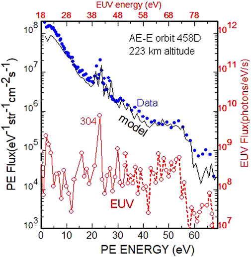
FIGURE 1. Measured (dots) and modeled (solid black line) photoelectron flux at 223 km. The red solid and dashed lines show the F74113 solar EUV reference irradiance as a function of energy, which has been shifted down by 18 eV (top axis) to approximately line up the EUV photons with the primary photoelectrons that they produce. The dashed line irradiances are double those of the standard F74113 irradiances.
Ideally, a model calculation should match the photoelectron flux magnitude well at the peaks and also at most other energies up to 60 eV. Beyond 60 eV the low instrument count rate introduces a lot of measurement uncertainty. A model should also reproduce the altitude variation of the photoelectron flux well as the dominant species changes from N2 to O. If the model does not match the overall flux magnitude, it should at least match the shape of the spectrum.
A key insight of Richards and Torr (1981) was that the 20–30 eV peaks have only a small contribution from the cascade process. That insight greatly simplifies the flux calculation below ∼250 km where transport is negligible. So, the prominent peaks can be used to validate the complex full photoelectron calculations at these energies. The calculation using the observed F74113 304Å solar irradiance revealed that the best fit to the peaks is obtained with electron impact cross-sections that are approximately a factor of 2 smaller than most used previously. The problem could be solved if the measured photoelectron fluxes were a factor of 2 too high or the 304Å solar irradiance was a factor of 2 too small. The general opinion amongst modelers in the early 1980s was that the measured photoelectron fluxes were a factor of 2 too high. This was not borne out by later measurements and modeling.
In addition to validating the full flux calculation, the 1981 study revealed that the electron impact cross-sections that were used in prior calculations would create photoelectron flux spectra that did not match the shape of the measured spectra. With this observation, Richards and Torr (1984) decided to try to determine the energy variation of the electron impact cross-sections that would be needed to reproduce the shape and magnitude of the observed photoelectron fluxes. As revealed below, these results published in 1984 identified a problem with the F74113 standard solar EUV irradiance for wavelengths below 250Å (see dashed line in Figure 1).
The technique was to recast the photoelectron problem by using the measured solar EUV irradiance and photoelectron fluxes to determine the total electron impact cross-sections for O and N2 that would be compatible with those measurements. The O cross-section was determined from ionosphere data around 250 km where O is the dominant species and the N2 cross-section was determined below ∼200 km where N2 is the dominant species. Both the O and N2 cross-sections so obtained were only about half of the other sets of cross-sections that were being used at the time in photoelectron models.
A more concerning problem was that there was a distinct discontinuity near 35 eV in both the O and N2 cross-sections that were calculated from the ionosphere data. The curve labeled AE in Figure 2 shows the discontinuity for the N2 electron impact cross-section. The oxygen electron impact cross-section had a similar discontinuity. The calculated cross-sections increase smoothly as expected from the threshold near 15 eV to about 35 eV. Then both cross-sections drop to only half of their prior value. This behavior is contrary to the well-established shape of the laboratory cross-sections in this energy range (solid line). Since the discontinuity occurred in both the O and N2 cross-sections, Richards and Torr (1984) suggested that the F74113 solar EUV irradiance was a factor of 2 too small below 250Å. Private consultations with Hans Hinteregger confirmed that the solar irradiances below 250Å were the least reliable in the F74113 solar EUV spectrum. So, it was decided to double the solar EUV irradiance below 250Å (dashed line in Figure 1) for all subsequent calculations of ionosphere densities and temperatures. Although there was a problem with the magnitude of the F74113 irradiance below 250Å, the variation with changing solar activity proved to be satisfactory, which allowed accurate scaling of all wavelengths with solar activity.
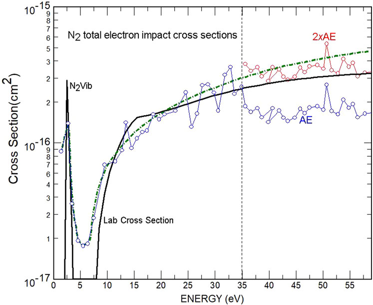
FIGURE 2. Comparison of N2 cross-sections derived from Atmosphere Explorer solar EUV irradiance and photoelectron flux (AE) with Laboratory cross-section (solid line). The dash-dot line is a weighted least-squares fit to the 1.0xAE data points below 35 eV. The points labeled 2xAE were obtained by doubling the AE values. The label N2Vib identifies the cross-section peak near 2.5 eV that results from vibrational excitation of N2.
When the cross-section results were submitted for publication, the unconventional technique resulted in a good deal of pushback from two reviewers and a third reviewer was consulted. He was a laboratory scientist involved with N2 cross-section measurements and was concerned that we might be casting aspersions on the laboratory measurements. After a phone conversation, he became convinced that this result was important because it identified a serious problem with solar EUV irradiance, and the paper was finally published. It turned out to be one of the two most important papers that we published. From this experience, I adopted a policy of never reviewing journal articles anonymously. It has led to some productive and enjoyable interactions with authors.
After the paper was published, the modified F74113 solar irradiances were used in all our ionosphere calculations of densities and temperatures for the next 10 years until 1993 when a reviewer challenged their use in a paper concerned with the comparison of our calculated ion densities and temperatures with measurements. That criticism prompted the development and publication of the EUVAC solar irradiance model that has been widely used (Richards et al., 1994). The EUVAC model is based on the F74113 solar EUV irradiances with the doubling of the solar irradiance short ward of 250Å. It was not until almost 20 years after its initial discovery that the problem with the F74113 solar irradiance was confirmed by new measurements from the Student Nitric Oxide Explorer (SNOE) satellite (Bailey et al., 2000). Further confirmation came from the measurements of the SEE experiment on the TIMED satellite (Woods and Eparvier, 2006).
Despite these corroborating measurements, skepticism continued in the general aeronomy community. When I took up a position as a program scientist at NASA headquarters in 2003, I worked with fellow program scientist, Bill Peterson, who expressed skepticism about the Richards and Torr photoelectron work. To settle the issue, we decided to compare model calculations with his photoelectron data from the FAST satellite. The model-data agreement was highly satisfactory, and our subsequent collaboration led to 11 journal articles on various aspects of photoelectron behavior (e.g., Richards and Peterson, 2008; Peterson 2021). These papers show that the 2-stream photoelectron model not only produces good agreement with photoelectron data in the local ionosphere but also in the plasmasphere including backscattered fluxes from the conjugate ionosphere.
Although great progress has been made in photoelectron flux and ionosphere theory, there are still unresolved problems. None of the current solar irradiance models adequately capture the photoelectron flux variations (Peterson et al., 2012). To date, photoelectron modeling has not been tested with a truly comprehensive set of coincident high-resolution measurements of both photoelectron and solar EUV spectra.
Inadequate knowledge of the photoelectron and EUV spectra is likely the reason that ionosphere models routinely underestimate the E-region peak electron density by > 30% (Solomon et al., 2001). Photoelectrons are the major source of ions and electrons in the E-region. Because the chemical loss rate is a square function of the electron density, a 30% model-data difference could correspond to a factor of 2 underestimate of the photoelectron source. Resolution of this problem would require coincident high-resolution rocket measurements of the photoelectron spectra and high-resolution measurements of the solar EUV X-ray spectrum, along with ion and neutral densities.
Epilogue
The collaboration with Bill Peterson that began at NASA HQ illustrates the scientific importance of taking full advantage of being in the right place at the right time. My career has benefited from several other fortuitous circumstances that have led to a deeper understanding of the space environment. Photoelectron modeling played a central role in the research examples below.
Among these happenstances was a decision in 1971 to get a degree at LaTrobe University. There, I was adopted as a graduate student by the well-known pioneering space physicist professor Keith Cole who was very supportive. His reputation helped me to obtain a post-doc at the University of Michigan with Doug Torr in May 1978 where Andy Nagy introduced me to his 2-stream photoelectron code. For some reason, Doug had great faith in my ability and set challenging research goals that greatly expanded my scientific horizons. At the University of Michigan Space Physics Research Laboratory in those days, it was common practice to submit a meeting abstract before the investigation had even started, possibly as a motivator for post-docs to work long hours. Fortunately, we usually managed to avoid embarrassing performances at meetings.
One such example was the submittal of an abstract in August 1979 for a meeting in Canberra, Australia to be held in December 1979. The abstract described the reevaluation of the solar EUV heating efficiency, which entailed the daunting work of updating the model to include a photoelectron calculation, comprehensive photochemistry, and additional dynamics of minor species. The solar EUV heating efficiency was important for efficient neutral gas heating calculations in global thermosphere models. These heating efficiency calculations were CPU intensive and had to be done remotely on the CRAY-1 computer located in Boulder CO. Just before getting on the plane to Australia the results were output on line-printer paper and the EUV heating efficiency was evaluated using a calculator on the flight to Australia. Our EUV heating efficiencies were different from previous ones in important ways but were later confirmed by others.
On another occasion, chance discussions in a hallway at the 1990 fall American Geophysical Union meeting led to a solution to a vexing problem for ionosphere modeling. By then, the basic ion chemistry had been established from laboratory and Atmosphere Explorer satellite measurements. However, there was great uncertainty in the ion dynamics because of a lack of knowledge of the thermosphere neutral winds that affect the modeled electron density and temperature. It is not possible to accurately model the electron density profile without first accurately reproducing the observed hmF2. The neutral wind determines the height of the ionosphere peak electron density (hmF2). Without an accurate thermal electron density profile, the heating by photoelectrons was not accurate and therefore the electron and ion temperature could not be modeled accurately either. The key insight was to have an ionosphere model assimilate hmF2 as a proxy for the neutral wind (Richards, 1991). The peak height and peak density (NmF2) have been well-measured globally for many decades using ground-based ionosondes. An algorithm was developed to modify the neutral winds to cause the model to closely follow the observed hmF2 automatically as it stepped in time. Just as with the early photoelectron work, this procedure was greeted with much skepticism but has now become widely accepted. Together with the earlier EUV and photoelectron work, this algorithm enabled more accurate studies of the electron density and temperature as a function of altitude. The neutral winds produced by the algorithm are also a useful by-product of the algorithm, greatly increasing the amount of neutral wind data available for other studies.
Another fortuitous collaboration that connected all these ideas together occurred in 1996 during a 3-months sabbatical visit to LaTrobe University. Peter Dyson’s group had only just finished extracting high-quality hmF2 and NmF2 data from their ionosonde. They also had accurate optical measurements of the neutral wind and temperature. These data enabled a detailed test of the photoelectron and EUVAC models and the neutral wind algorithm (Dyson et al., 1997; Richards et al., 1998).
There remain some vexing problems in ionosphere modeling. While the modeling of the quiet midlatitude F-region ionosphere is now reasonably mature, more dynamic conditions at high and equatorial latitudes and during geomagnetic storms still present a major challenge primarily due to the difficulty in accounting for the rapid changes in the key inputs such as neutral densities and winds, and electric fields. It is likely that data assimilation will be necessary for further improvement of the modeling of these more dynamic conditions and that will require improved data availability on smaller scales.
Data availability statement
The data analyzed in this study is subject to the following licenses/restrictions: No restrictions. The data are available from the author. Requests to access these datasets should be directed to Phil Richards, cGdyaWNoZHNAZ21haWwuY29t.
Author contributions
PR performed all research on this perspective and wrote the manuscript.
Conflict of interest
The authors declare that the research was conducted in the absence of any commercial or financial relationships that could be construed as a potential conflict of interest.
Publisher’s note
All claims expressed in this article are solely those of the authors and do not necessarily represent those of their affiliated organizations, or those of the publisher, the editors and the reviewers. Any product that may be evaluated in this article, or claim that may be made by its manufacturer, is not guaranteed or endorsed by the publisher.
Acknowledgments
The author thanks the colleagues mentioned in this article as well as the many colleagues in the space science community who supported and critiqued my research. Special thanks to Andy Nagy who generously shared his photoelectron model and expertise and to Bill Peterson for being a great collaborator and for reviewing this article prior to submission.
References
Bailey, S. M., Woods, T. N., Barth, C. A., Solomon, S. C., Canfield, L. R., Korde, R., et al. (2000). Measurements of the solar soft X-ray irradiance by the Student Nitric Oxide Explorer: First analysis and underflight calibrations. J. Geophys. Res. 105 (27), 27179–27193. doi:10.1029/2000ja000188
Dyson, P. L., Davies, T. P., Richards, P. G., Parkinson, M. L., Reeves, A. J., Fairchild, C. E., et al. (1997). Thermospheric neutral winds at southern mid-latitudes: A comparison of optical and ionosondehmF2methods. J. Geophys. Res. 102, 27189–27196. doi:10.1029/97ja02138
Hinteregger, H. E. (1981). Representations of solar EUV fluxes for aeronomical applications. Adv. Space Res. 1, 39–52. doi:10.1016/0273-1177(81)90416-6
Nagy, A. F., and Banks, P. M. (1970). Photoelectron fluxes in the ionosphere. J. Geophys. Res. 75, 6260–6270. doi:10.1029/ja075i031p06260
Peterson, W. K. (2021). Perspective on energetic and thermal atmospheric photoelectrons. Front. Astron. Space Sci. 8. doi:10.3389/fspas.2021.655309
Peterson, W. K., Woods, T. N., Fontenla, J. M., Richards, P. G., Chamberlin, P. C., Solomon, S. C., et al. (2012). Solar EUV and XUV energy input to thermosphere on solar rotation time scales derived from photoelectron observations. J. Geophys. Res. 117, A05320. doi:10.1029/2011JA017382
Richards, P. G. (1991). An improved algorithm for determining neutral winds from the height of the F2 peak electron density. J. Geophys. Res. 96, 17839. doi:10.1029/91ja01467
Richards, P. G., Dyson, P. L., Davies, T. P., Parkinson, M. L., and Reeves, A. J. (1998). Behavior of the ionosphere and thermosphere at a southern midlatitude station during magnetic storms in early March 1995. J. Geophys. Res. 103 (26), 26421–26432. doi:10.1029/97ja03342
Richards, P. G., Fennelly, J. A., and Torr, D. G. (1994). EUVAC: A solar EUV flux model for aeronomic calculations. J. Geophys. Res. 99, 8981. doi:10.1029/94ja00518
Richards, P. G., and Peterson, W. K. (2008). Measured and modeled backscatter of ionospheric photoelectron fluxes. J. Geophys. Res. 113, A08321. doi:10.1029/2008JA013092
Richards, P. G., and Torr, D. G. (1981). A formula for calculating the theoretical photoelectron fluxes resulting from the He+ 304 Å solar spectral line. Geophys. Res. Lett. 8, 995–998. doi:10.1029/gl008i009p00995
Richards, P. G., and Torr, D. G. (1984). An investigation of the consistency of the ionospheric measurements of the photoelectron flux and solar EUV flux. J. Geophys. Res. 89, 5625. doi:10.1029/ja089ia07p05625
Solomon, S. C., Bailey, S. M., and Woods, T. N. (2001). Effect of solar soft X-rays on the lower ionosphere. Geophys. Res. Lett. 28, 2149–2152. doi:10.1029/2001gl012866
Keywords: ionosphere, thermosphere, photoelectrons, solar EUV, cross-sections
Citation: Richards PG (2022) Ionospheric photoelectrons: A lateral thinking approach. Front. Astron. Space Sci. 9:952226. doi: 10.3389/fspas.2022.952226
Received: 24 May 2022; Accepted: 30 June 2022;
Published: 22 July 2022.
Edited by:
Joseph E. Borovsky, Space Science Institute, United StatesReviewed by:
Tamas I. Gombosi, University of Michigan, United StatesMichael Denton, Space Science Institute, United States
Copyright © 2022 Richards. This is an open-access article distributed under the terms of the Creative Commons Attribution License (CC BY). The use, distribution or reproduction in other forums is permitted, provided the original author(s) and the copyright owner(s) are credited and that the original publication in this journal is cited, in accordance with accepted academic practice. No use, distribution or reproduction is permitted which does not comply with these terms.
*Correspondence: P. G. Richards, cGdyaWNoZHNAZ21haWwuY29t