Towards an AI-based understanding of the solar wind: A critical data analysis of ACE data

1 Introduction

The space weather community aims to understand and quantify the associated threats, mitigate them, and in the best cases, prevent them altogether. Recently, Daglis et al. (2020) detailed a new scientific program of the Scientific Committee on Solar-Terrestrial Physics (COSTEP) called PRESTO, for Predictability of the variable Solar-Terrestrial coupling. Such a study highlighted the remaining questions surrounding the understanding of the Sun-Earth coupling. Among these open questions, we can find:

• How do various solar wind conditions (e.g., IMF components, speed, density, level of turbulence) and different large-scale drivers control the coupling efficiency and the energy/mass transfer from the solar wind to the magnetosphere?

• How do solar wind conditions control the occurrence frequency and location of different magnetospheric plasma waves?

These questions emphasize the role of the solar wind as it is indeed one of the key issues in the predictability of the Earth space environment. Studies to better understand both solar wind and the interplanetary magnetic field using coordinated space- and ground-based data along with models are of essential importance. Recently, the emergence of machine learning algorithms in space weather Camporeale et al. (2018), Camporeale (2019), Camporeale (2020) appeared as one of the most promising solutions to nowcast and forecast phenomena in space weather. More and more papers using machine learning, and especially deep learning, are published in the field of space weather Reiss et al. (2021), Zewdie et al. (2021), Stumpo et al. (2021), Reep and Barnes (2021).

Initiated in 2018, a Research Coordination Network (RCN) supported by the National Science Foundation (NSF) named “Towards Integration of Heliophysics Data, Modelling, and Analysis Tools” (@HDMIEC) planned to make progress in the understanding of physical mechanisms in the Sun and on modelling and the data accessibility and analysis. In this regard, workshops, and discussions around the topic of Machine Learning in Space Weather were held and the opinion of the community was gathered. Several outcomes from the Q&A sessions are worth to be noticed from Nita et al. (2020):

• Half of the attendees (46.7%) agreed that the heliophysics community does not even have a fair understanding of machine learning capabilities and limitations.

• There was a consensus that cooperation between ML and heliophysics does not exist.

• ML methods are more successful regarding the Big Data environment behind heliophysics than physics-based methods. But there is no consensus around which areas could ML methods outperform physics-based ones.

• The overwhelming majority of attendees strongly agreed (73.3%) that there is a need to combine physics-based and ML models.

• Most of the attendees did not feel that the ML was a “bubble” ready to burst.

In this paper, we decided to discuss the use of solar wind data in the context of artificial intelligence. Firstly, because the solar wind is a central data as seen through PRESTO. Secondly, because most of the space weather community is not so familiar with AI and its good practices but seems ready to use it more in the future Nita et al. (2020). Hence, we present here a complete data analysis of the ACE solar wind and IMF measurements, an essential and largely used data when forecasting on-Earth events, even today (Myagkova et al. (2020), Wintoft et al. (2015), etc.). While we will not expand on this in this paper, it is interesting to notice that a lot of studies use the NASA’s OMNIWeb dataset (see https://omniweb.gsfc.nasa.gov/html/ow_data.html) such as Wihayati et al. (2021) or Gombosi et al. (2018) for instance. High-Resolution OMNIWeb data are made of ACE, IMP 8, Wind and Geotail satellites data gathered and time-shifted to the Bow Shock Nose. Although they are really interesting data, we did not want to add here any complexity through the fact that this time-shifting was based on several asumptions and needed an intercalibration between satellites. This data preparation is largely documented on OMNIWeb (https://omniweb.gsfc.nasa.gov/html/HROdocum.html).

These kinds of analyses are “required to correct for scattering, baselines changes, peak shifts, noises, missing values and several other artefacts so that the “true” relevant underlying structure can be highlighted and/or, if required, the property of interest can be predicted correctly” Mishra et al. (2020). The chosen data go from 1998 to 2021, including a large part of the 23rd and the full 24th solar cycles (for a schematic view, see the Supplementary Figure S1, showing the Solar radio flux index at 10.7 cm, a good representation of the solar activity). The objective of this paper is to extract all possible useful information that can be found in solar wind data and highlight the issues that could arise when applying machine learning algorithms and techniques.

Before diving into the subject, it is worth noticing that impressive work has been done by Smith et al. (2022) on a similar topic. Their paper consists of an analysis of the quality and continuity of the data that are available in Near-Real-Time from the Advanced Composition Explorer and Deep Space Climate Observatory (DSCOVR) spacecraft. Part five (Discussion and Conclusion) of our work details how our two studies differ.

2 A quick introduction to machine learning concepts

In order to better understand the data analysis presented here, we first need to quickly introduce some concepts in Machine Learning. According to Oxford Dictionary, Machine Learning is “the use and development of computer systems that are able to learn and adapt without following explicit instructions, by using algorithms and statistical models to analyse and draw inferences from patterns in data”. The products include models, forecasts, identification of patterns, anomalies, or even relationships among data. Machine learning is usually described through two categories of algorithms: supervised learning and unsupervised learning (although it exists a wealky-supervised algorithm that embraces both ideas).

• Supervised learning LeCun et al. (2015) includes regression algorithms and classification algorithms. The first aims at discovering connections between input and output data and is often employed to approximate functions or predict future values of continuous functions. It comprises linear regressions, decision trees, most of neural networks, and ensemble methods, among others. The second aims at mapping input data to classes and is therefore usually employed to classify data (e.g., True/False problems). It includes support vector machines (SVM), discriminant analysis, naïve Bayes classifiers, and K-nearest neighbour, among others. Such algorithms are called supervised because they require to be fed examples of output data to train.

• Unsupervised Learning Storrs et al. (2021) includes clustering algorithms, which group data together. Clustering algorithms map input data to a set of categories initially identified by the system (e.g., Gaussian Mixture Model, K-mean). They are referred to as unsupervised because one does not know their output. A simple example is the grouping of customer profiles, where the final quantity of groups is unknown at first.

The procedure is often the same: access, scrap, analyse and pre-process the data (format, missing values, etc.), choose and compute the features that will be used for the model and train the model thanks to a loss function taking or not the label into account (subjective choice from the user). We then iterate the last three steps to find the best model. As introduced in this paper, the key and most time-consuming parts are the data analysis and the pre-processing, as we need to build a scalable and efficient ready-to-use dataset to answer a given problem. The pre-process ends with a split of our data into three groups:

• The train set: a dataset that will be used by our algorithm to train itself.

• The validation set: a dataset used by the algorithm to test itself. The accuracy of the model on this dataset allows the user to see how good it is at predicting, how fast and how well it is training and allows him to make some changes accordingly.

• The test set: a dataset that will never be used by the user and the model until the very last moment. The user applies his trained and ready-to-use model to this dataset to ultimately know the final accuracy of his model and to avoid a human/user bias from hyperparameter tuning.

Finally, it is worth noticing that the train and validation sets have to be “well-balanced”. This means that all possible cases should appear in both datasets and, ideally, in the same quantities. A model will easily get used to recurrent cases. If we only have one or two samples of fast solar wind in our train set, and thousands of slow solar wind samples, the model will not be able to accurately predict fast-solar wind cases. One possibility to address this issue is to perform what we call data augmentation, but we will not expand it here Shorten and Khoshgoftaar (2019), Chen et al. (2020).

3 Data description

The Advanced Composition Explorer (ACE) satellite is located in the Lagrange point 1 (L1), a stable point in space, between the Earth and the Sun, where the gravitational attraction from both bodies and the centrifugal force all balance each other. Satellites at this location are at the front line to see phenomena coming from the Sun.

ACE Solar Wind Data are Level-2 Real-Time Solar Wind (RTSW) data. “Level 2” means that raw data from the instruments have been processed by the instrument teams. According to the Ace Science Center Level 2, it includes such operations as calibration, organization into energy and time bins, or application of ancillary data. The frequency of measurements for instruments MAG (Magnetometer) and SWEPAM (Solar Wind Electron Proton Alpha Monitor) are respectively 16-s and 64-s, from 1998 to 2020. The data have been gathered from the following link: srl. caltech.edu/ACE/ASC/level2/where they are considered to be official and verified¹. A lot of research needing solar wind data also uses OMNIWeb 1-min and 5-min solar wind datasets mathematically time-shifted from the Lagrange one point to the Earth’s bow shock nose King and Papitashvili (2006). Choosing these manually propagated data as input to nowcast or forecast near-Earth data Shprits et al. (2019), McGranaghan et al. (2021), Bentley et al. (2018) is a good idea to prevent a machine-learning-made propagation which can be subject to unidentified errors. However, as the point of this paper is to highlight the dangers of using in situ data, it was more relevant to take in situ solar wind values.

We focus on the data from two main instruments of the ACE satellite:

• SWEPAM McComas et al. (1998), for Solar Wind Electron, Proton and Alpha Monitor measures rates of electron and ion flows with two distinct electrostatic analyzers with fan-shaped fields of view that use the spacecraft’s rotation to observe in all directions. The first one observes electrons in the 1 eV–1.35 keV energy range and the second one ions in the 0.26–36 keV energy range. For this instrument, we only focus on ion data, spanning 23 years from 1998 to 2020 with a 64-s resolution. This corresponds to 11, 299, 710 measurements.

• MAG, for Magnetic Field Monitor, consists of a set of twin sensors (triaxial fluxgate magnetometers, Stone et al. (1998)) measuring the three components of the interplanetary magnetic field at L1. For this instrument, we have 25 years of 16-s data from 1997 to 2021. We removed the years 1997 and 2021 to have the same time range as the SWEPAM instrument. In the end, we have 45, 365, 393 data points for this instrument. For the first part of our analysis, we decided to subsample the dataset every 64 s. With both years removed, we obtain 11, 341, 349 measurements. However, the corresponding times of each sample do not correspond to SWEPAM’s ones, and another post-process (presented further) had to be done to compare data between the two instruments.

Here are the analyzed in situ measurements and their unit:

• IMF X, Y and Z-component, GSE coordinates [nT]

• Solar wind proton density [cm⁻³]

• Solar wind proton speed [km.s⁻¹]

• Solar wind ion temperature [K]

For the interplanetary magnetic field, X, Y and Z-component are in the GSE (Geocentric Solar Ecliptic) coordinates instead of the GSM. By definition Russell (1971) the X-axis points from the Earth towards the Sun, the Y-axis is chosen to be in the ecliptic plane opposing the planetary motion, and the Z-axis is parallel to the ecliptic pole. This system has been chosen instead of GSM because the aberration of the solar wind due to the orbital motion of Earth around the Sun representing a 30 km/s vector oriented in the minus Y direction axis is easier to remove Russell (1971). According to Russell (1971), GSE coordinates have been widely used to display satellite trajectories, interplanetary magnetic field observations, and solar wind velocity data.

4 Data analysis

In this part, we present the full analysis along with related conclusions.

• In the first part, statistical distributions of the data are plotted and explained, and every variable will be looked at independently of others. In all the datasets, there are some missing values that perturb the statistics computations. We removed all of them in this first part.

• The second part is an example of how to handle the aforementioned missing and extreme values.

• The third part will study the classical linear relationships between the different variables. Aside from being important to better understand our data, it is worth reminding that too many intercorrelated input features may give redundant information to an AI algorithm and then lower its performance. The topic of interdependencies in solar wind data has already been looked at in the literature (e.g., in Bentley et al. (2018)) but will be done here in the light of neural networks and deep learning.

4.1 Linear analysis of the IMF, and Plasma’s parameters

Before studying neural networks, it is important to begin with a simple linear analysis. Theses analysis allow to reveal some important information and features about data with simple computations which will help you save a lot of time during the deep learning study.

Observing various parameters of the Solar Wind and the interplanetary field gives us a good insight into their nature. The first step is to look at their histogram and statistical parameters such as mean, median, maximum or the standard deviation, globally, yearly and potentially in a shorter time period. Both solar wind and the IMF are influenced by the solar activity which evolves on 11-year cycles. Recall that all the statistics in this part are computed on non-missing values only.

It is essential to understand how values can fluctuate, evolve, or change in time when we are dealing with time series. The following Table 1 highlights two interesting things: the great number of missing values in SWEPAM data, and the large distance between the 99.995th percentiles and mean values for Bt and the Ion Temperature. Such spread values seem dangerous to implement in a deep-learning algorithm without a pre-process.

TABLE 1

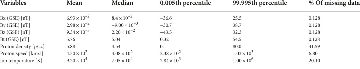
TABLE 1. Mean, median, 0.005th and 99.995th percentile from ACE MAG and SWEPAM data.

Figure 1A shows the yearly standard deviation of the three components of the IMF. It is a direct witness to the obvious the dependencies of some of our parameters over the solar cycle because it follows the global trend of the solar activity index F10.7 throughout the year. All possible figures to detect dependence of distribution parameters over time have been plotted. Only some of them are shwon in this paper.

FIGURE 1

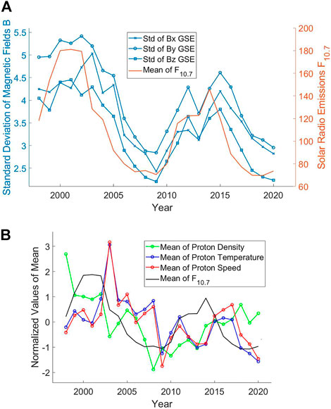
FIGURE 1. (A) Standard deviations per year of the three-components of the interplanetary magnetic field (Bx, By, Bz) in GSE coordinates compared to the mean per year of the solar radio flux at 10.7 cm from NASA’s OMNIWeb (omniweb.gsfc.nasa.gov/)—1998 to 2020. Values are not normalized here. (B) Mean of Proton Density, Temperature, Speed and Solar Radio Index F10.7 per year, from 1998 to 2020. All values are normalized (center 0 and standard deviation 1) to plot them on the same scale.

Figure 1B is another example of how values can change over time and shows that the evolution of the yearly average temperature and speed of the solar wind already suggests a dependence between the two. In other words, different periods in our dataset imply different distributions depending on the solar activity. Although it may seem obvious for a space weather expert, it is information of prime importance for the data scientist dealing with these datasets. Such observations suggest that the solar activity in the name of F10.7 has to be part of the inputs as we will have to know where we are in the solar cycle. Moreover, this highlights the need to have at least one full solar cycle in our training set to span all possible cases.

4.1.1 Histograms

Distributions are essential for the data scientist to assess the information contained in a dataset. For instance, under-represented values will have a more important high error on average than most-represented values. Although a limited number of plots are shown here, all histograms have been plotted and analyzed.

4.1.1.1 SWEPAM

Most of SWEPAM variables distributions (i.e., plasma parameters) were close to lognormal distributions Burlaga and Lazarus (2000). Hence, for clarity purposes and to enhance our understanding, we also plot the distribution of the logarithm applied to these varaibles.

Ion velocity is the only plasma parameter that differs from a lognormal distribution. The most probable value is 364 km s⁻¹, lower than its median value 408 km s⁻¹. Most conclusions from Veselovsky et al. (2010) still hold when adding all the data until 2021. Although solar wind speed can reach values such as 1,000 km s⁻¹, 94.2% of all values are contained in the 300 km s⁻¹ to 700 km s⁻¹ window. Moreover, 500 km s⁻¹ seems to be a breaking point, suggesting that two different distributions could overlap with a local maximum of around 600 km s⁻¹. According to Burlaga and Lazarus (2000), this could be due to corotating interactions regions where fast solar wind catches up slow solar wind, when corotating streams from coronal holes are numerous. As these phenomena appear more during declining solar activity, we plotted distribution for 2002–2009, 2015–2020 (two cumulated declining phases of solar activity) and distribution on the remaining dates (ascending phases). If needed as a comparison, the full distribution can be observed in the Supplementary Figure S2.

Figures 2A, B confirm a 600 km s⁻¹ peak during the declining phases of the solar activity, as suggested by Burlaga and Lazarus (2000) with data from 1995 to 1998 (here confirmed with new data from 1998 to 2020). If we approximate the distribution of speed as lognormal, it then appears that the two declining phases of the solar activity are adding a Gaussian distribution of speed centered around 580–600 km s⁻¹. This is confirmed when looking at Figure 8 in Xu and Borovsky (2015). They classified solar wind into four plasmas: coronal-hole-origin plasma, streamer-belt-origin plasma, sector-reversal-region plasma, and ejecta. We see in Figure 2A the coronal-hole-origin plasma (black arrow). Let’s keep in mind that a lot of work is being done to have the solar wind classified (e.g., Camporeale et al. (2017)). This information is of prime importance if we want to use the solar wind to forecast other parameters.

FIGURE 2

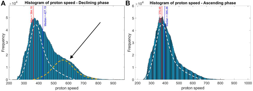
FIGURE 2. (A) Distribution of ion speed (km.s⁻¹) between 01 January 2002 and 22 October 2009 and between 23 October 2014 and 09 September 2019 corresponding to declining phases of the solar activity. (B) Distribution of ion speed for opposite periods (km.s⁻¹), corresponding to ascending phases of the solar activity. The maximum of the distribution (i.e., the most probable value) and median are also plotted on the two figures. The white dotted lines are an approximation of the shape of the distribution during the ascending phase (2b), while the yellow dotted line represent the potential contribution of the coronal-hole-origin plasma with a peak at 600 km s⁻¹ (pointed by the black arrow).

Proton density follows a lognormal distribution with the most probable value being 2.94 cm⁻³ (Figures 3A, B). As seen Figure 1B, this value is highly influenced by the solar cycle. The peak of the density distribution is moving through our 23-years period, roughly following the solar cycle (represented here by F10.7 averaged each year).

FIGURE 3

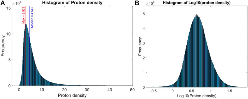
FIGURE 3. (A) Distribution of ion density (cm⁻³). Red line highlights the maximum of the curve or most probable value (equals to 2.939 cm⁻³) and the blue line highlights the median value (equals to 4.542 cm⁻³). (B) Distribution of logarithmic (base 10) values of the proton density.

Unlike Burlaga and Lazarus (2000), we do not observe any double peak in our ion density distributions, and our most probable value is far from their 8.0 cm⁻³ value (our is approximately 2.94 cm⁻³). One can imagine this to be related to the global decline in solar activity since solar cycle 22 (solar cycles can be seen in the Supplementary Figure S1) but we do not have a proper explanation. This suggests, again, that we should not use less than 11 years of data to train our algorithm (ideally at least three cycles).

Temperature is well approximated by a lognormal distribution, and the most probable value is around 30,000 K. The two distributions have a similar shape to the ones in Figure 3 (if needed, this can be seen in the Supplementary Figure S4 for normal and logarithmic histograms). However, our computation of the most probable value shows an offset to the right instead of representing the peak of the distribution. This is one of the major issues that we will have with SWEPAM data in general, mentioned in Veselovsky et al. (2010): rounding of numbers is performed to different orders, with different significant digits. To highlight this issue, we plotted another histogram of the ion temperature with a higher number of bins (1,000,000) and zoomed on corresponding zones (Figure 4). As an example, when the temperature reaches 10,000K, the measures start to be rounded every 1 K (instead of every 0.1 K for values below 10,000 K). The same goes when reaching 100,000K, the measures start to be rounded every 10 K. The distribution when taking the logarithm values of the ion temperature is an even better view of the “jumps” in scale. Although these changes are anecdotic in most astrophysical applications, they are far from negligible in the AI context. Such changes in scale multiply the amount of data having identical values (as seen in Figure 4, where the maximum is shifted to the right). Yet, a deep-learning algorithm will wrongly interpret these values as being more probable and will give them more importance during the training although they are not supposed to be so (maximum probability of temperature should stay around 30,000 K). As a consequence, the algorithm will only focus on the most-probable value and the others will not be able to lead to coherent and correct results.

FIGURE 4

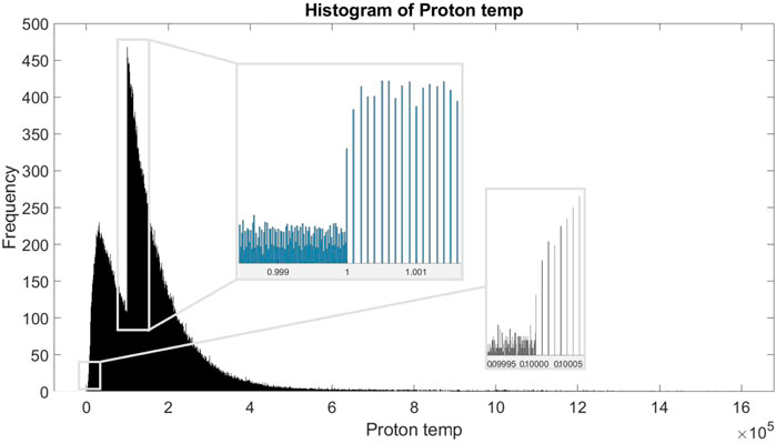
FIGURE 4. Same histogram of ion temperature than S.4 using 1,000,000 bins. Figure is zoomed on two specific zones, highlighting the changes in order of magnitude when rounding the measures.

4.1.1.2 MAG

Histograms of the X, Y, and Z-components of the IMF seem close to Gaussian distributions. The norm of the IMF magnetic field vector seems close to a lognormal distribution. All plots can be found in the Supplementary Figures S5−S8). Some observed characteristics:

• X and Y-components could be interpreted as two superposed Gaussian, with two different most probable results each. X and Y components seem to have opposite values and are linked by the orientation of the IMF when coming from the Sun (i.e., magnetic field lines are either oriented towards or away from the Sun). In addition, plotting the median of all values each year for these components suggest also suggests a strong relationship between the two, that should be considered before implementing them as input. The yearly median of both distributions seems to evolve in opposite directions over time and this is in line with the investigation shown in part 4.3. (report to part 4.3. for a better understanding but this can still be checked Supplementary Figure S3).

• The Z-component of the IMF is strangely following a perfect Gaussian curve with a center close to 0. Without any additional information from the space weather scientific community, one might assimilate the Z-component to a white-noise signal i.e., consider Bz as random. However, it is known (see for example Kivelson et al. (1995)) that the Bz-component orientation is responsible for magnetic reconnection at the front of the magnetosphere. When pointing southward, the IMF can connect to the Earth’s northward magnetic field, allowing plasma to enter the dayside magnetosphere. When using ACE data to nowcast or forecast possible impacts of solar phenomena on in-space and on-ground systems, it is not possible to exclude the Bz-component. In general, analyzing data to answer a specific need using Machine Learning cannot be properly done without including the physical systems and phenomena responsible for the observations. The physics lying behind the data has to be addressed and understood to avoid absurd solutions and errors.

• Finally, the total IMF—B— distribution seems very close to a Laplacian distribution.

As a conclusion on histograms:

• Data shown here cannot be put in the algorithm as such. Distributions are everything but uniform and will lead to unequal training over samples. A possible consequence is having an algorithm incapable of dealing with rare cases (tails of the Gaussian and Laplacian curves).

• Gaussian noise is inherent to instruments. It might be very difficult (but useful) to evaluate the signal-to-noise ratio. A possible consequence on the training loss curve is to observe a steep drop followed by a flat trend, meaning that the algorithm quickly trained on the information it has and then started training on noise.

• Relation (linear or not) between data cannot be overlooked (we investigate them in part 4.3.).

• Particular attention is required on data values, as shown by the changes in the order of magnitude in the ion temperature (which, furthermore, could not be seen without manually increasing the number of bins).

4.1.2 Autocorrelations

The autocorrelation function (ACF) gives the data analyst indications on how future values are influenced by past values in time series. It helps identify randomness or periodic patterns, seasonality, and trends. When plotting ACF on the different features here, no autocorrelation is noticed, except for two trends.

• IMF norm, X and Y-components reveal a 27-day periodicity, corresponding either to the Carrington synodic rotation period of the Sun or the Bartels Rotation Number. Solar rotation varies with latitude, with a maximum of 38 days at the poles and less than 25 days at the equator. In this context, the synodic period is 27.2753 days Wilcox (1972), and the Bartels Rotation Number is chosen to be exactly 27 days Bartels (1934) (the number of apparent rotations of the Sun as viewed from Earth and from L1 in our case).

• IMF norm also reveals the 11-year solar activity cycle.

• Density, temperature, and speed reveal the same two periodicities.

Graphs do not bring enough information and will just appear in the Supplementary Figures S9−S12 for the reader’s curiosity. It is important to notice that the lack of a clear autocorrelation is good news to apply machine learning technics. Time series data tend to be autocorrelated by having consecutive data with quite similar values. The risk when trying to forecast the next value is to end up using a persistence model, where the algorithm just picks the last value as being the best approximation for the next one. This is avoided when we have almost no autocorrelation, which is our case here.

4.2 Missing and extreme values

Missing and extreme values is a real struggle when working on AI algorithms but are more than usual in the Space Weather field. Table 1 also presents the percentages of missing data in our dataset and Figure 5 represents through a black and white image the missing values in our dataset. On the left side of Figure 5 are the MAG measurements and on the right side are the SWEPAM measurements. At a glance, we can see that the time tags for missing values in the interplanetary magnetic field are the same, meaning that the instrument measures the components of the IMF altogether and that one missing value on a component means missing values on all components.

FIGURE 5

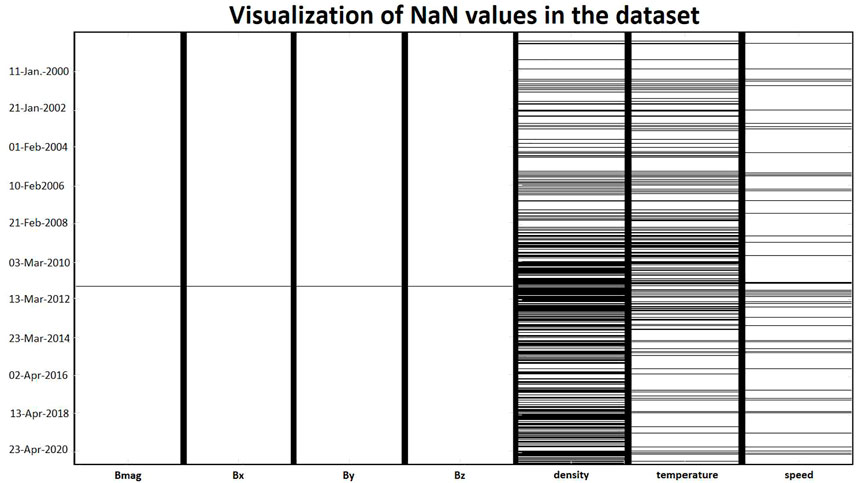
FIGURE 5. Visualization of missing values (i.e., NaN—Not a Number) in the dataset. Each black and white column here represent all values of one variable (see x-axis). Each line of pixels within these columns represent the presence (horizontal white lines) or absence (horizontal black lines) of values for a given datetime (y-axis). All dataset is shown from first to last datetime, every 64 s. These maps help quickly visualize when in time are the missing values and which parameter is the most affected.

What we noticed from MAG does not hold for SWEPAM. Although most of the missing data happen at the same moment, they are still not distributed in the exact same way. However, it seems like when speed is missing, all of them are. This type of visualization is easy to create, and very useful to make a first opinion on how missing values are organized (in which variables, around which year, etc.).

Finally, there are much more missing data in the SWEPAM dataset than in the MAG one, and almost half of the proton density data is missing: a very high amount that cannot be ignored when dealing with AI. Such high percentages require that we take a closer look as done in Figure 6 (and, later, in Table 2).

FIGURE 6

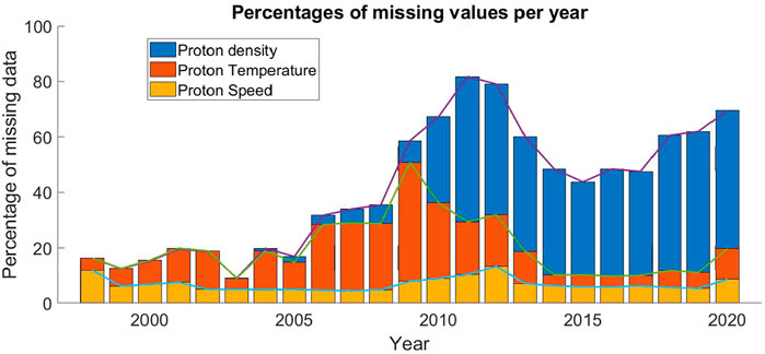
FIGURE 6. Percentage of data that are missing in the SWEPAM measurements (i.e., proton speed, proton density, and proton temperature) per year, from 1998 to 2020.

TABLE 2

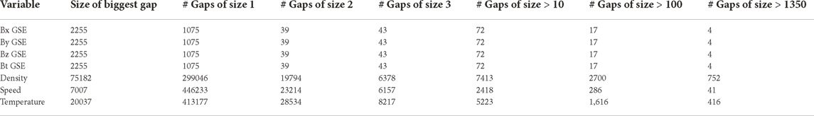
TABLE 2. Size of the biggest gap (number of consecutive missing values in the data) and number of gaps having a certain size (e.g., size 1 = one missing data surrounded by non-missing values, size 3 = 3 consecutive missing data) in the X, Y and Z-components of the IMF, and in the solar wind density, speed and temperature.

Data here are Level-2 data, meaning that a group of experts analyzed them and kept reliable measures. Starting from 2009/2010, the amount of missing data is greatly increasing. This information seen in Figure 6 is confirmed when looking at the data status update of the ACE Science Center on 23 October 2012:

“The SWEPAM observations, in particular the proton density and to a lesser extent the temperature, became increasing sparse starting in 2010 as the primary channel electron multiplier (CEM) detectors have aged. […] In response, the ACE science team has developed and implemented, starting 23 Oct 2012, an innovative mission operations concept that more frequently repoints the ACE spacecraft’s spin axis further away from the Sun.” (Skoug et al. (2012)).

This information is of high value for Machine Learning scientists. As we saw, when working with an AI algorithm, we split the data into a train, a validation, and a test dataset. What is usually done in AI applied to Space Weather (and even broader when dealing with time series) is to pick a whole period (e.g., an entire year) as the validation or test set McGranaghan et al. (2021). A random choice would be dangerous as we might end up with a year with 81% of missing values (e.g., 2010).

The next question to answer is how these missing values will be processed. First, let’s check the gaps of consecutive missing data and their size.

Table 2 shows the variety of gaps in our data. The biggest gap in the SWEPAM instrument is made of 75,182 consecutive missing data, approximately 55.6 consecutive days in the proton density. The density also has 752 gaps longer than a day. The longest gap in the speed is 5.2-day long, and the longest gap in the temperature is almost 15-day long. They have respectively 41 and 416 gaps more than 24 h long. Once again, we confirm the issue already seen for the density and temperature measurements: more than a lot of missing data, there are a lot of consecutive missing data.

Concerning the interplanetary magnetic field, this table also goes in the same direction as Figure 5. It confirms that the missing data are at the same time for all components of the magnetic field: only four gaps longer than a day and the longest gap is approximately 40-h long. Several processes exist to deal with missing data. Here are some examples:

• Removing all the rows containing missing data. The main advantage of this method is the robustness of the resulting model. However, using this method usually also removes some non-missing data. Here, the total loss of rows will be based on the ion density’s data, as it has 41.51% of missing data. It will result in a loss of almost four million proton speed data and 2.4 million proton temperature data points.

• Imputing missing values (especially for time series) with mean, median, last seen value, or through linear, spline or other interpolations. Such methods are quite easy to implement but might result in unplausible results. In the following (Figures 10, 11), we applied the spline interpolation (as seen in some literature concerning AI in Space Weather - e.g., Gruet (2018)) on a few hours’ gaps in our SWEPAM’s ion temperature data around November 2020.

Figure 7B represents Figure 7A with gaps filled with spline interpolation. As expected, a spline interpolation cannot be used when a gap is too large, it fills the dataset with values at different orders of magnitudes. The risk lies in the divergences such as the one between 13 August and 20 August 2009, giving very high values compared to the initial curve that now seems flat. Such extreme values will highly disturb algorithms, especially neural networks and can restrain them from learning. Even more, neural networks will tend to give high importance to these values, that were not even in our dataset at first.

However, it is efficient with smaller gaps in (around 10 to 15 missing values according to Andriambahoaka (2008)). The gaps seen in Figure 8A between 28 August and 30 August 1998, are good examples on how efficient the spline interpolation can be for small gaps. Figure 8B shows the result when interpolating with spline.

FIGURE 7

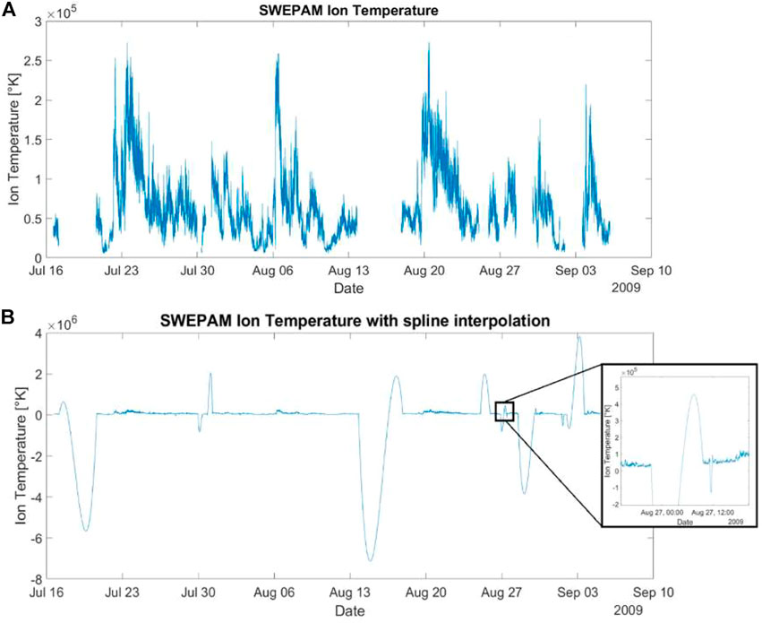
FIGURE 7. (A) SWEPAM’s Ion Temperature from the 16th of July to the 10th of September 2009. This period has been chosen to evaluate the efficiency of using spline interpolation when we have large gaps in the data. (B) SWEPAM’s Ion Temperature from the 16th of July to the 10th of September 2009. Gaps seen in Figure 7A are now filled using a spline interpolation. On the right is a zoom on a particular period to highlight the large divergence caused by the interpolation.

FIGURE 8

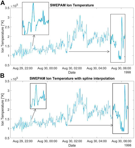
FIGURE 8. (A) SWEPAM’s Ion Temperature from 28 August to 30 August 1998. This period has been chosen to evaluate the efficiency of using spline interpolation when we have small (here minutes-long) gaps in the data. We zoomed on two of them for easier observation. (B) SWEPAM’s Ion Temperature from the 28th of August to the 30th of August 1998. Gaps seen in Figure 8A are now filled using a spline interpolation. We zoomed on the same two periods for easier observation.

It is essential to keep in mind this dependence on gaps’ sizes when trying to impute values to missing data. The best way to deal with it is to have a detailed analysis of missing data (as we saw in Table 2, or in Figures 5, 6), and use the best available method by first isolating characteristic gaps and testing methods on them independently.

• Finally, it is worth noticing that in astrophysics, gaps in the data could be filled by using other instruments and satellites that are measuring the same variables. In our case, satellites such as DSCOVR, also located in L1, represent viable solutions. However, inter-calibration between instruments will then have to be double-checked and can become critical if not considered.

As a conclusion on missing values:

• Missing data cannot be left aside and have to be looked at and processed, especially when dealing with time series.

• An analysis of the missing data should at least include percentages per variable, amount of missing data in time, size and number of gaps, few plots along with the data. It is advised to also consult the data suppliers and experts to better understand the analysis.

• While a large number of processes exist (e.g., removing rows or interpolating), they are not equivalent, and their use should depend on the aforementioned dataset analysis.

4.3 Interdependencies between variables

After analyzing every data independently, we now focus on comparing them together through three assessments:

• Two-dimensional statistical distributions

• Correlation matrices

• Principal Component Analysis

4.3.1 Two-dimensional statistical distributions

We analyzed the two-dimensional statistical distributions of values for the logarithm of the solar wind’s speed, temperature, and velocity. We are using the logarithm as an answer to the lognormal distributions observed in part 4.1.1.1. Here are the figures for speed and temperature (Figure 9A) and for speed and density (Figure 9B). The distribution for temperature and density did not highlight anything interesting.

FIGURE 9

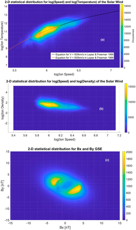
FIGURE 9. (A) 2-D statistical distribution for logarithmic (base 10) values of solar wind speed and logarithmic (base 10) values of solar wind temperature. The two curves (respct. red and black) are the empirical equations from Lopez and Freeman (1986) (respectively for a solar wind speed smaller and greater than 500 km s⁻¹). (B) 2-D statistical distribution for logarithmic (base 10) values of solar wind speed and logarithmic (base 10) values of solar wind density. (C) 2-D statistical distribution for the X and Y-components of the IMF [nT] from MAG data.

These 2D statistical distributions highlighted well-known results:

• Proton temperature increases with solar wind speed and a linear correlation appears between the two (Figure 9A). In 1986, this linear correlation has been approximated by Lopez and Freeman (1986) with a difference for speeds above and below 500 km s⁻¹. We verified the accuracy of their following equations in the graph:

$T=\left(0.77\pm 0.021\right)V-\left(265\pm 12.5\right)\text{for\hspace{0.17em}}V>500km.s^{-1}(1)$

$T^{0.5}=\left(0.031\pm 0.002\right)V-\left(4.39\pm 0.08\right)\mathrm{f}\mathrm{o}\mathrm{r}V<500km.s^{-1}(2)$

The first one appears in black in Figure 9A while the second appears in red. It is interesting to notice that a model built in 1986 seems quite valid on these data from 1998 to December 2020. During CMEs however, temperature is usually lower Richardson and Cane (1995).

• Density and speed are well correlated. Fast solar wind is usually less dense, and slow solar wind varies a lot Geiss et al. (1995). Recall that fast solar wind can catch up slow solar wind and compress it creating what is called corotating interaction regions Jian et al. (2006). This is a known result but the corresponding figure is shown here (Figure 9B)

Concerning MAG, the two-dimensional statistical distribution for the X and Y-components of the IMF has two maxima and shows the approximate 45° angle between the IMF vector and the radial Sun-Earth direction. This angle is the direct consequence of the characteristic Parker’s spiral (first theoretically predicted by Chapman) flow of the solar wind Parker, 1963; Kivelson et al. (1995). These two maxima can be found in Figure 9C. Two-dimensional plots including the Bz were not adding new information and are not shown here.

4.3.2 Linear correlation matrices

Until now, we subsampled MAG data to obtain one data point every 64 s. Now, to compare MAG and SWEPAM together, it is important to have the same timestamp for every data. The choice made was to keep SWEPAM data and its corresponding timestamps and, for every data point of SWEPAM, take the closest MAG 16sec-data point in time and change its timestamp to the SWEPAM’s one². The result is a dataset of 11, 282, 160 data points, from the 04th of February 1998 to the 22nd of December 2020. After removing all rows where data were missing, we end up with 6,559,840 samples from which we can compute the correlations and the corresponding p-values matrices (Figure 10).

FIGURE 10

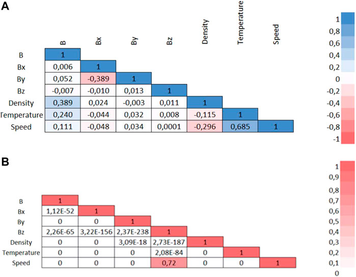
FIGURE 10. Matrices of correlation (A) coefficients for the IMF absolute value and its three components (from ACE’s MAG instrument) and the three parameters (speed, density and temperature) of the solar wind (from ACE’S SWEPAM instrument) and the corresponding p-values (B). p-values range from 0 to 1, where closed-to-zero values 0 mean the corresponding correlation coefficient is significant (or that there is a low probability of observing the null hypothesis, meaning the correlation coefficients are not random).

As expected, the correlations between the proton’s speed and temperature, and between density and temperature (although smaller) appear. Two small negative correlations (between proton’s speed and density and between X and Y-components of the IMF) also appear. Oddly enough, there is a high p-value for the correlation coefficient between speed and the Z-component of the IMF, but the correlation is inexistent (Figure 10). Finally, let’s recall that the correlation coefficient is none other than the cosine of the angle between the two centered vectors and that the cosine function is not linear. Hence, a 0.685 (our higher correlation coefficient here) corresponds to a 46.76° angle between the two vectors. In other words, no significant enough correlation has been obtained here. From an AI point of view, and without nonlinear pre-processing, this means that we want to keep all the parameters as they might contain different relevant information. But would it be possible to combine parameters together to reduce the total amount of parameters needed? The principal component analysis will answer this question.

4.3.3 Principal component analysis (PCA)

What is the idea behind the PCA? As an example, let’s assume that we have a dataset made of p different variables and let’s suppose that each observation is close to a specific n-dimension hyperplane in ${\mathbb{R}}_p(n\le p)$. The idea of the PCA is to find this possible “best plane” (the plane such that the sum of the distances of the points to that plane is the smallest). PCA then gives us this new coordinate system (or affine space of dimension n) and data are projected in it. Note that the distances between observations in this new system best reflect the distances between observations in the starting space ${\mathbb{R}}_p$. PCA answers the problem of finding the n-dimensional linear space which best represents the observations in the sense that the orthogonal projection on this space moves them as little as possible. In AI, it is widely used when preprocessing the data either to reduce the number of features needed or to target the most relevant features in a given dataset.

Following in Figure 11 is the PCA applied to our dataset (IMF |B|, X, Y and Z-components, proton density, temperature, and speed). In the output of the PCA are the principal components, which are the vectors of the new coordinate system. The first component is such that it contains the greatest variance of some scalar projection of the data points on it. For further understanding, a handmade example (for which data have nothing to do with ours) can be seen in the Supplementary Figure S13.

FIGURE 11

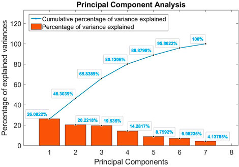
FIGURE 11. Percentage of explained variance for each principal component from the principal component analysis (in red bins) of the 7 parameters (|B|, X, Y and Z-components of the IMF, solar wind speed, density and temperature) and the cumulative percentage value in blue.

Hence, from Figure 11, it appears that the PCA does not find any good coordinate system in which to project the data points, justifying the use of more complex models for data analysis and data processing (e.g., non-linear models, Hinton’s t-distributed stochastic neighbour embedding—Van der Maaten and Hinton (2008)). This can be seen in the quasi-linear augmentation of the cumulative percentage of variance explained. An ideal case would have been to have a major (90%) percentage of the variance explained by the first three principal components but almost all components here explain the same amount of variance.

As a conclusion on dependencies between variables:

• There is a dependency between speed and temperature that will need further observations.

• There is a non-linear relationship between the X and the Y-components of the IMF. Hence, they cannot be considered independently.

• Most of the graphs did not show any linear dependency (this will be checked further with correlation matrices) and hence might imply the use of non-linear models. This has been confirmed by the correlation matrix and the PCA.

5 How to use the data for AI

Once we observed and analyzed the data, we need to preprocess it, which usually means:

• Choosing the final set of input features and labels. The selection of variables to pass as input into the model is essential. The model must be informed of the possible relationships between inputs and outputs. Some information might not be sufficient for the model to understand these relationships and it is then highly recommended to discuss the underlying objectives with experts from the field. In astrophysics problematics, the physical relationships between variables have to be used to construct the set of features McGranaghan et al. (2021). However, too many features carrying the same information might also impact the performance of the model. It is better to avoid redundant information Khalid et al. (2014). Intercorrelations and PCA are quite useful to remove some unwanted features. Moreover, the final samples will be built as a vector containing all the input features and the label (labelled data appear in supervised learning algorithms only) and, in the case of time series, one has to choose the temporal resolution for it (usually the resolution of the labels). Features with a lower resolution will have missing values and features with a higher resolution will be transformed (e.g., mean, max, standard deviation, etc.). Indeed, the set of features can include transformed variables (e.g., the square of the density). Of course, it might also contain passed values of variables (e.g, the magnetic field B, and the same magnetic field B 1 hour ago, or 1 day ago). In this case, autocorrelations are useful to identify redundant information in time. Overall, choosing the input features will depend on our objectives (whether it is forecasting or classifying for example) and our knowledge of the underlying physical phenomena (depending on our aims, the algorithm might find better solutions with the density squared or with the past 3 h of magnetic field).

• Handling the missing values. Null values are quite a challenge as they are abundant in the space weather field. Removing entire rows of data will result in significant information loss, and we just saw that interpolation depends on the sizes of gaps in the data. In our context, a good response might be to find another satellite or data source when talking with experts (e.g., DSCOVR) and fill the gaps using interpolation with these new data points. If we do not have other data sources, a compromise should be found between removing and interpolating.

• Standardizing or normalizing the data. We will not detail here the differences between these two, but rescaling the data is required for the model to compare inputs together. It avoids placing too much emphasis on variables with large values (e.g., speed would be considered more important than density). The field of astrophysics also faces observations with high variance and a large number of outliers (defined as extreme values far from the initial distribution, often thought to be generated by a different mechanism–Hawkins (1980)). Outliers are particularly problematic when located in the labels of the dataset. The extent to which a label-outlier disrupts the training will be discussed in a subsequent paper. One way to remove these outliers is to remove entire samples where labels are behind certain quantiles in their probability distribution. For instance, McGranaghan et al. (2021) removed all samples where the labels’ values were out of the 99.995th percentiles. However, in space weather we are often concerned about the extreme values since they pose the most risk. A user must be able to differentiate between real anomalies and extreme values that are accouting for extreme phenomenon and treat them differently. The algorithm cannot distinguish them by itself. Another possibility would be to do anomaly detection (another field of Machine Learning) but, again, it is impossible to assess the efficiency of the algorithm without an expert able to differentiate anomalies and relevant exteme values. Finally, a user could adapt the loss function to account for physical phenomenon. Loss functions are functions allowing the algorithm to learn, they are cost function Wang et al. (2022) such as the Mean Squared Error function. The difficulty in adapting a loss function is that one must very well understand the physics behind the phenomena, but trying to understand these phenomena is often the very point of using AI in the first place.

6 Discussion and Conclusion

In the field of Space Weather, the use of AI is progressively gaining importance. First mentions of machine learning techniques or neural networks at the European Space Weather Week appeared around 2011 and dedicated “Machine learning and statistical inference techniques” sessions only appeared in 2016. In this context, proper understanding and pre-processing of the data is central. Here, we decided to focus on ACE satellite data as it has been widely used by the community and considered a good indicator to forecast the near-Earth phenomena. Its location (L1) and measurements (IMF, solar wind parameters and particle fluxes) made it the perfect candidate for our study. Obviously, the methods presented here have to be adjusted depending on the dataset and one’s objectives. Concerning our dataset, the conclusions are the following:

• Some parameter distributions are well approximated by Gaussian distributions while others are closer to lognormal laws. As said in Veselovsky et al. (2010) lognormal laws can testify of “multiple multiplicative transformations of local characteristics at intermitting random intensifications and attenuations of waves, compression and rarefaction of irregularities in turbulent processes of transporting mass, energy, and momentum on the Sun and in the heliosphere”. Overall, histograms are not uniform distributions at all. If we use data as such, algorithms will perform well on more frequent samples and poorly on rare cases. For example, if the purpose is to forecast events related to very fast and dangerous solar winds, our algorithm will struggle to obtain anything interesting. Moreover, it is important to keep in mind the possible noise in our measurements. The signal-to-noise ratio seems difficult to estimate here and the interesting information may be hidden in noisy data.

• Histograms are not steady and change from year to year, maybe due to dependence to the solar cycle. This means that a model built on a single (or limited number of) year(s) might not be reproducible and usable in the future. At best, one should know the origin of such changes. In any case, the training set has to be well-balanced and has to include several different years of data (e.g., both ascending and descending phases of the solar cycle).

• We must pay special attention to rounded measurements when there are changes in the order of magnitude within the data, as seen with the ion temperature data. The consequence could be an over-attention of the algorithm on higher values as they would appear more frequent. Two possible solutions here: either round all the data to the highest order of magnitude, or artificially re-distribute values following the closest Gaussian distribution (when looking at the logarithm of proton temperature).

• The number of missing values in our dataset is significant and has to be addressed (e.g., 41.59% of proton density data missing). For the analysis, we removed the corresponding samples, but it is not a solution for the training when the number of missing values is very high. The best solution here would be to use DSCOVR data. Either way, when filling missing data, sizes of gaps have to be looked at to choose a corresponding interpolation method for instance.

• Even if we noticed the well-known linear relationship between speed and temperature of the solar wind, a linear model might not be enough to accurately model the data. It seems that non-linear relationships between data exist (e.g., X-component and Y-component of the interplanetary magnetic field). PCA, correlation matrix and 2-D statistical distributions suggest that all parameters should be kept and that non-linear models should be preferred.

• Overall, some cycles appear in the dataset. Proton speed seems highly dependent on the solar cycle and the synodic rotation period of the Sun appears in most of the autocorrelations. We advise having several solar cycles included in the training set to avoid biases. Solar cycle could also be part of our input features through the solar radio flux at 10.7 cm or the sunspots number.

As mentioned in the introduction, Smith et al. (2022) study is very complementary to ours. The differences lie in the methods and data chosen.

• First, Smith et al. (2022) take into account both ACE and DSCOVR data while we only focused on level-2 ACE data.

• They compare together Near-Real-Time (NRT) raw data to the same data post-processed by the scientific community. On our side, we do not assess the quality and relevance of raw data as we considered level-2 data as the entry point of any AI study in this field. Smith et al. (2022) indeed show that the NRT values are subject to short-term variability and anomalous values, confirming our choice.

• Concerning missing values, Smith et al. (2022) again compare NRT and scientific data. They draw some conclusions about the amount data gaps, but we go slightly beyond in Table 2 and through the testing of filling methods. However, their analysis on windowed data validity (part 3.2.2.) is very interesting. Indeed, some AI algorithms need windows of consecutive data (e.g., Temporal Convolutional Network) to learn properly. Here, as shown in their study: “if 2 hours (120 min) of continuous input are required then […] approximately 1% of plasma data are available.” Missing values is then an even bigger problem and it is required to choose a method to deal with missing values.

• Finally, concerning autocorrelations, the difference lies in the use of data. Smith et al. (2022) do autocorrelations on NRT data and only on 1 h-long windows of consecutive data without missing values. On our side, we do autocorrelations on level-2 ACE data and we take all the data as input and omit the computation for missing values.

Data analysis goes hand in hand with the field’s expertise. Some of the solutions suggested here will not be ideal depending on one’s objectives and the conclusions one might have when looking only at the statistics could also be wrong. As an example, even if Gaussian distributions are often associated with random processes, we know that the mechanisms lying behind the values of the IMF and solar wind are everything but random. We also know that very fast and powerful CMEs can saturate instruments and create missing values, hence changing how we would consider replacing them. Knowing how AI algorithms work can give us clues on what to focus on when analyzing a dataset and where a problem might arise. However, it is the understanding of these data and a space weather expertise together that will allow us to favor one solution over another.

Data availability statement

Publicly available datasets were analyzed in this study. This data can be found here: https://izw1.caltech.edu/ACE/ASC/level2/.

Author contributions

SB: Conceived and designed the analysis; Collected and organized the data; Contributed data or analysis tools; Contributed astrophysics analysis; Performed the analysis and created graphs; Wrote the paper PV: Contributed to the data science part of the analysis; Conceived and designed the analysis; Contributed data or analysis tools; Helped writing paper; Contributed to the redaction with major corrections and changes MB: Contributed to the astrophysics part of the analysis; Corrected several parts of the manuscript JC: Correction and guidance All authors contributed to manuscript revision, read, and approved the submitted version.

Acknowledgments

The authors would like to acknowledge the ACE Science Center for providing the data and especially Andrew Davis for answering our concerns. In addition, the authors would like to thank Data Science Expert and the PNST (Programme National Soleil-Terre). A special thanks to Pierre Porchet for his precious help in understanding, processing, and drawing conclusions from the data. Special thanks to Elisa Robert and Angélique Woellflé for their support and expertise. The authors would also like to thank SpaceAble for their support and expertise. The company was not involved in the study design, collection, analysis or interpretation of data.

Conflict of interest

Author SB was employed by SpaceAble.

The remaining authors declare that the research was conducted in the absence of any commercial or financial relationships that could be construed as a potential conflict of interest.

Publisher’s note

All claims expressed in this article are solely those of the authors and do not necessarily represent those of their affiliated organizations, or those of the publisher, the editors and the reviewers. Any product that may be evaluated in this article, or claim that may be made by its manufacturer, is not guaranteed or endorsed by the publisher.

Supplementary material

The Supplementary Material for this article can be found online at: https://www.frontiersin.org/articles/10.3389/fspas.2022.980759/full#supplementary-material

Footnotes

¹A special thanks to Andrew Davis from the ACE Science Center for his answers and advice on the use of data.

²Special thanks to Pierre Porchet and his generous help in preparing this massive dataset (processing 45 million data points for MAG and 11 million for SWEPAM - respectively 6.3 and 2.6 Gigabytes of data).

References

Andriambahoaka, Z. (2008). “Modélisation régionale du champ magnétique terrestre et établissement de cartes magnétiques détaillées appliqués à Madagascar,” (Strasbourg, France: Université Louis Pasteur). Ph.D. thesis.

Google Scholar

Bartels, J. (1934). Twenty-seven day recurrences in terrestrial-magnetic and solar activity, 1923–1933. J. Geophys. Res. 39 (3), 201–202a. doi:10.1029/TE039i003p00201

CrossRef Full Text | Google Scholar

Bentley, S., Watt, C., Owens, M., and Rae, I. (2018). ULF wave activity in the magnetosphere: Resolving solar wind interdependencies to identify driving mechanisms. J. Geophys. Res. Space Phys. 123 (4), 2745–2771. doi:10.1002/2017JA024740

CrossRef Full Text | Google Scholar

Burlaga, L., and Lazarus, A. (2000). Lognormal distributions and spectra of solar wind plasma fluctuations: Wind 1995–1998. J. Geophys. Res. 105 (A2), 2357–2364. doi:10.1029/1999JA900442

CrossRef Full Text | Google Scholar

Camporeale, E., Carè, A., and Borovsky, J. E. (2017). Classification of solar wind with machine learning. J. Geophys. Res. Space Phys. 122 (11), 10–910. doi:10.1002/2017JA024383

CrossRef Full Text | Google Scholar

Camporeale, E.S. O. C. of ML-Helio (2020). ML-Helio: An emerging community at the intersection between heliophysics and machine learning. JGR. Space Phys. 125 (2), e2019JA027502. doi:10.1029/2019JA027502

CrossRef Full Text | Google Scholar

Camporeale, E. (2019). The challenge of machine learning in space weather: Nowcasting and forecasting. Space weather. 17 (8), 1166–1207. doi:10.1029/2018SW002061

CrossRef Full Text | Google Scholar

Camporeale, E., Wing, S., and Johnson, J. (2018). Machine learning techniques for space weather. Amsterdam, Netherlands: Elsevier.

Google Scholar

Chen, S., Dobriban, E., and Lee, J. H. (2020). A group-theoretic framework for data augmentation. J. Mach. Learn. Res. 21 (1), 9885–9955. doi:10.48550/arXiv.1907.10905

CrossRef Full Text | Google Scholar

Daglis, I., Chang, L., Dasso, S., Gopalswamy, N., and Khabarova, O. (2020). Predictability of the variable solar-terrestrial coupling. Annales Geophysicae. doi:10.5194/angeo-39-1013-2021

CrossRef Full Text | Google Scholar

Geiss, J., Gloeckler, G., and Von Steiger, R. (1995). Origin of the solar wind from composition data. Space Sci. Rev. 72 (1), 49–60. doi:10.1007/BF00768753

CrossRef Full Text | Google Scholar

Gombosi, T. I., Chen, Y., Manchester, W., Zou, S., Hero, A. O., Landi, E., et al. (2018). Machine learning and the” holy grail” of space weather forecasting. SM54A–02.

Google Scholar

Gruet, M. (2018). “Intelligence artificielle et prévision de l’impact de l’activité solaire sur l’environnement magnétique terrestre,” (Toulouse, ISAE. Ph.D. thesis.

Google Scholar

Hawkins, D. M. (1980). Identification of outliers. Berlin, Germany: Springer.

Google Scholar

Jian, L., Russell, C., Luhmann, J., and Skoug, R. (2006). Properties of stream interactions at one AU during 1995–2004. Sol. Phys. 239 (1), 337–392. doi:10.1007/s11207-006-0132-3

CrossRef Full Text | Google Scholar

Khalid, S., Khalil, T., and Nasreen, S. (2014). “A survey of feature selection and feature extraction techniques in machine learning,” in Proceedings of the 2014 Science and Information Conference, London, UK, 27-29, Aug. 2014, 372–378. doi:10.1109/SAI.2014.6918213

CrossRef Full Text | Google Scholar

King, J., and Papitashvili, N. (2006). One min and 5-min solar wind data sets at the Earth’s bow shock nose. Greenbelt, Md: NASA Goddard Space Flight Cent.

Google Scholar

Kivelson, M. G., Kivelson, M. G., and Russell, C. T. (1995). Introduction to space physics. Cambrindge, United Kingdom: Cambridge University Press.

Google Scholar

LeCun, Y., Bengio, Y., and Hinton, G. (2015). Deep learning. nature 521 (7553), 436–444. doi:10.1038/nature14539

PubMed Abstract | CrossRef Full Text | Google Scholar

Lopez, R. E., and Freeman, J. W. (1986). Solar wind proton temperature-velocity relationship. J. Geophys. Res. 91 (A2), 1701–1705. doi:10.1029/JA091iA02p01701

CrossRef Full Text | Google Scholar

McComas, D., Bame, S., Barker, P., Feldman, W., Phillips, J., Riley, P., et al. (1998). “Solar wind electron proton alpha monitor (SWEPAM) for the Advanced Composition Explorer,” in The advanced composition explorer mission (Berlin, Germany: Springer), 563–612. doi:10.1007/978-94-011-4762-020

CrossRef Full Text | Google Scholar

McGranaghan, R. M., Ziegler, J., Bloch, T., Hatch, S., Camporeale, E., Lynch, K., et al. (2021). Toward a next generation particle precipitation model: Mesoscale prediction through machine learning (a case study and framework for progress). Space weather. 19 (6), e2020SW002684. doi:10.1029/2020SW002684

CrossRef Full Text | Google Scholar

Mishra, P., Biancolillo, A., Roger, J. M., Marini, F., and Rutledge, D. N. (2020). New data preprocessing trends based on ensemble of multiple preprocessing techniques. TrAC Trends Anal. Chem. 132, 116045. doi:10.1016/j.trac.2020.116045

CrossRef Full Text | Google Scholar

Myagkova, I., Shirokii, V., Vladimirov, R., Barinov, O., and Dolenko, S. (2020). “Comparative efficiency of prediction of relativistic electron flux in the near-earth space using various machine learning methods,” in International conference on neuroinformatics (Berlin, Germany: Springer), 222–227. doi:10.1007/978-3-030-60577-325

CrossRef Full Text | Google Scholar

Nita, G., Georgoulis, M., Kitiashvili, I., Sadykov, V., and Camporeale, E., 2020. Machine learning in heliophysics and space weather forecasting: A white paper of findings and recommendations. arXiv preprint arXiv:2006.12224. 10.48550/arXiv.2006.12224.

Google Scholar

Parker, E. N. (1963). The Solar-Flare Phenomenon and the Theory of Reconnection and Annihiliation of Magnetic Fields. The Astrophysical Journal Supplement Series 8, 177

CrossRef Full Text | Google Scholar

Reep, J. W., and Barnes, W. T. (2021). Forecasting the remaining duration of an ongoing solar flare. Space weather. 19 (10), e2021SW002754. doi:10.1029/2021SW002754

CrossRef Full Text | Google Scholar

Reiss, M. A., Möstl, C., Bailey, R. L., Rüdisser, H. T., Amerstorfer, U. V., Amerstorfer, T., et al. (2021). Machine learning for predicting the Bz magnetic field component from upstream in situ observations of solar coronal mass ejections. Space weather. 19 (12), e2021SW002859. doi:10.1029/2021SW002859

CrossRef Full Text | Google Scholar

Richardson, I., and Cane, H. (1995). Regions of abnormally low proton temperature in the solar wind (1965–1991) and their association with ejecta. J. Geophys. Res. 100 (A12), 23397–23412. doi:10.1029/95JA02684

CrossRef Full Text | Google Scholar

Russell, C. T. (1971). Geophysical coordinate transformations. Cosm. Electrodyn. 2 (2), 184–196.

Google Scholar

Shorten, C., and Khoshgoftaar, T. M. (2019). A survey on image data augmentation for deep learning. J. Big Data 6 (1), 60–48. doi:10.1186/s40537-019-0197-0

CrossRef Full Text | Google Scholar

Shprits, Y. Y., Vasile, R., and Zhelavskaya, I. S. (2019). Nowcasting and predicting the K p index using historical values and real-time observations. Space weather. 17 (8), 1219–1229. doi:10.1029/2018SW002141

CrossRef Full Text | Google Scholar

Skoug, R., Mccomas, D., and Elliott, H. (2012). Effect of ACE spacecraft repointing on SWEPAM calculated moments.

Google Scholar

Smith, A., Forsyth, C., Rae, I., Garton, T., Jackman, C., Bakrania, M., et al. (2022). On the considerations of using near real time data for space weather hazard forecasting. Space weather. 20 (7), e2022SW003098. doi:10.1029/2022sw003098

CrossRef Full Text | Google Scholar

Stone, E. C., Frandsen, A., Mewaldt, R., Christian, E., Margolies, D., Ormes, J., et al. (1998). The advanced composition explorer. Space Sci. Rev. 86 (1), 1–22. doi:10.1023/A:1005082526237

CrossRef Full Text | Google Scholar

Storrs, K. R., Anderson, B. L., and Fleming, R. W. (2021). Unsupervised learning predicts human perception and misperception of gloss. Nat. Hum. Behav. 5 (10), 1402–1417. doi:10.1038/s41562-021-1097-6

PubMed Abstract | CrossRef Full Text | Google Scholar

Stumpo, M., Benella, S., Laurenza, M., Alberti, T., Consolini, G., and Marcucci, M. F. (2021). Open issues in statistical forecasting of solar proton events: A machine learning perspective. Space weather. 19 (10), e2021SW002794. doi:10.1029/2021SW002794

CrossRef Full Text | Google Scholar

Van der Maaten, L., and Hinton, G. (2008). Visualizing non-metric similarities in multiple maps. Mach. Learn. 9 (11), 33–55. doi:10.1007/s10994-011-5273-4

CrossRef Full Text | Google Scholar

Veselovsky, I., Dmitriev, A., and Suvorova, A. (2010). Algebra and statistics of the solar wind. Cosm. Res. 48 (2), 113–128. doi:10.1134/S0010952510020012

CrossRef Full Text | Google Scholar

Wang, Q., Ma, Y., Zhao, K., and Tian, Y. (2022). A comprehensive survey of loss functions in machine learning. Ann. Data Sci. 9 (2), 187–212. doi:10.1007/s40745-020-00253-5

CrossRef Full Text | Google Scholar

Wihayati, , Purnomo, H. D., and Trihandaru, S, (2021). “Disturbance storm time index prediction using long short-term memory machine learning,” in 2021 4th International Conference of Computer and Informatics Engineering (IC2IE), Depok, Indonesia, 14-15 Sep. 2021 (IEEE), 311–316. doi:10.1109/IC2IE53219.2021.9649119

CrossRef Full Text | Google Scholar

Wilcox, J. M. (1972). “Divers solar rotations,” in Cosmic plasma physics (Berlin, Germany: Springer), 157–164. doi:10.1007/978-1-4615-6758-520

CrossRef Full Text | Google Scholar

Wintoft, P., Wik, M., and Viljanen, A. (2015). Solar wind driven empirical forecast models of the time derivative of the ground magnetic field. J. Space Weather Space Clim. 5, A7. doi:10.1051/swsc/2015008

CrossRef Full Text | Google Scholar

Xu, F., and Borovsky, J. E. (2015). A new four-plasma categorization scheme for the solar wind. J. Geophys. Res. Space Phys. 120 (1), 70–100. doi:10.1002/2014ja020412, Available at: https://agupubs.onlinelibrary.wiley.com/doi/pdf/10.1002/2014JA020412.

CrossRef Full Text | Google Scholar

Zewdie, G. K., Valladares, C., Cohen, M. B., Lary, D. J., Ramani, D., and Tsidu, G. M. (2021). Data-Driven forecasting of low-latitude ionospheric total electron content using the random forest and LSTM machine learning methods. Space weather. 19 (6), e2020SW002639. doi:10.1029/2020SW002639, Available at: https://agupubs.onlinelibrary.wiley.com/doi/pdf/10.1029/2020SW002639.

CrossRef Full Text | Google Scholar