Exploratory data analysis (EDA) machine learning approaches for ocean world analog mass spectrometry

1 Introduction

Future planetary spacecraft will be equipped with next-generation instruments producing more data than can be sent back to Earth, while facing severe operations and transmission limitations (e.g., communication delays, limited bandwidth, limited reconnaissance (Thompson et al., 2012), harsh environmental conditions, and limited resources such as CPU and onboard memory). Due to these communication challenges, the ability to autonomously detect signals of scientific interest onboard the spacecraft could greatly benefit these missions by enabling data prioritization, thus increasing mission science return from outer Solar System targets. Undoubtedly, in situ missions to more challenging targets such as Mercury, Venus, and ocean worlds (e.g., Europa, Enceladus, Triton) will demand an innovative approach to mission design and operations to maximize science return.

Within the last few decades, ocean worlds have become the targets of several future space exploration missions. The ocean worlds include some icy moons of Jupiter, Saturn, Uranus, Neptune, and several dwarf planets in which oceans exist or may have existed; they represent opportunistic targets to find extant life beyond Earth, and could be natural laboratories to study the prebiotic processes that led to the emergence of life on Earth. Missions to these targets must overcome limited power and communication windows, and long communication delays. Therefore, future planned and possible missions to icy ocean worlds in the next decades will require innovations in technology, especially to meet astrobiological goals.

To overcome such challenges to ocean worlds missions, we envision an agile science operations plan (Thompson et al., 2012) wherein the spacecraft and flight software work together for onboard analysis of the acquired science data to inform subsequent actions to take. Some operations will need to shift from the current teleoperated data collection to automated onboard analysis in order to reduce the need for ground-based analysis and decision-making processes, which will enable decreased downtime in science data collection and increased science return. We posit that developing such an “agile” and modular architecture would enable any future mission to adapt the architecture for its instrumentation and science goals. Agile science operations have been studied for primitive bodies and deep space exploration. Thompson et al. (2012) describes this capability for comet sample return missions due to needs for near real-time target analysis and characterization to select a safe and effective sampling scheme in the subsequent spacecraft operations. Chien et al. (2014) further investigates this potential through the development of onboard autonomy for imaging instruments (e.g., navigation cameras). The ideal operations plan would enable the spacecraft to collect science data and talk to each subsystem in order to prioritize resources to meet science goals while respecting engineering constraints. It would be organized as follows: 1) acquire scientific data, 2) analyze scientific data onboard, 3) detect prespecified features (variables, predictors or attributes) of interest, 4) decide next operations for generating new data acquisition based on prespecified priorities set by the science team, 5) update the operational plan to acquire new data based on prioritization. This strategy would not only enhance science return, but would also enable science “on-the-fly” and science in environments with poor or no communication.

Some of these capabilities have been developed or are in development. For planetary science missions, Mars has been the main target of various investigations of autonomy. These include the detection of dust devils and clouds on Mars using the Spirit and Opportunity Mars Exploration Rovers (MER) (Andres et al., 2008), as well as the Autonomous Exploration for Gathering Increased Science (AEGIS) system on the Mars Science Laboratory (MSL) mission to autonomously detect targets of interest using the ChemCam instrument (Francis et al., 2015; Francis et al., 2017). Ocean worlds have been targets for detection algorithms investigations, such as the research of Wagstaff et al. (2019) on the detection of thermal anomalies (hot spots), compositional anomalies, and plumes on Europa during flybys of the future Europa Clipper. Most of this research has focused on imaging techniques to develop autonomy for space missions, and on data treatment for dimensionality reduction strategies. In contrast, we focus on similar advancements for mass spectrometry data, a challenging field due to the large data volumes of individual spectra, and a field prime for development and maturation of autonomous capabilities. Indeed, several teams are working to develop such capabilities (e.g., Da Poian et al., 2022; Mauceri et al., 2022). Mauceri et al. (2022) investigated the compression of raw mass spectra of the capillary electrophoresis coupled to mass spectrometry (CE-MS) instrument for the ocean world’s life surveyor (OWLS) instrument suite. Crucial to developing such useful onboard tools is exploratory data analysis (EDA), which is a common practice in data science and machine learning that uses a range of statistical and unsupervised learning to understand patterns in data.

One of the main motivations for the exploration of icy ocean worlds is their potential habitability, making them prime candidates in the search for life in our Solar System. An invaluable tool to support this effort is mass spectrometry (MS). MS is a technique with a rich heritage in planetary missions ranging from Apollo 17, Mars Viking Lander, Cassini-Huygens, to Mars Science Laboratory (MSL), and is used to characterize the chemical composition of planetary rocks, ice, and atmospheres (Mahaffy, 1999). It enables the identification and quantification of molecules, macromolecules from samples, and the detection of ions within the samples due to their mass-to-charge ratio (m/z). Mass spectrometers produce high-dimensionality output data that can be difficult to analyze because of noise. For this purpose, data-driven tools can greatly benefit/contribute to mass spectrometry analysis in different processing steps (removing noise, filtering corrupt spectra, preliminary categorization for prioritization) and discovery-driven inquiry (Chou et al., 2021). Mass spectrometry enables a comprehensive approach in providing complex measurements of chemical composition, with more quantitative data such as isotopic ratios and elemental abundances, as well as the observation of possible biosignatures through physical and chemical characteristics such as elemental distributions and isotopic fractionations (Neveu et al., 2018).

Future icy ocean world missions will be equipped with highly developed mass spectrometers enabling isotope ratio measurements of the volatiles evolving from the exosphere (a very tenuous atmosphere) and from the plumes. A clear understanding of isotopic fractionation will be essential to evaluate potential isotopic biosignatures for future ocean worlds missions. For instance, the MAss Spectrometer for Planetary EXploration (MASPEX) onboard the Europa Clipper mission will be able to analyze the isotopic composition of volatiles (e.g., CH₄, H₂O, NH₄, CO₂, etc.) (Brockwell et al., 2016) during fly-bys of Europa. We not only have to assess the capabilities of MS instruments to perform this task during fly-bys, but also evaluate the potential ability of onboard software in future missions (e.g., Enceladus Orbilander) to autonomously pre-process and identify signals of higher interest to enable data transmission prioritization.

In this paper, we describe EDA relevant for development of future AI and ML tools for mass spectrometry (MS). Here we use isotope ratio mass spectrometry (IRMS) data analyzed from laboratory analogs of ocean worlds as a use case to demonstrate how EDA can be used to inform data processing for further algorithm development. We describe an analytics pipeline with data science techniques to better understand the dataset(s) under study before applying supervised machine learning (ML) algorithms to identify and characterize specific features from ocean worlds analogs volatiles. As a longer-term goal, we envision the concept of science autonomy (Theiling et al., 2020; 2022; Da Poian et al., 2022) where data analysis processes–some of which are discussed in the current study–could be used onboard a spacecraft to conduct real-time data analysis and decision-making, and prioritize data transmission for bandwidth-limited outer Solar System missions, which could greatly enhance the science relevance of the limited data returned to Earth. This paper is not meant to be an exhaustive presentation of ML and data science tools for space exploration missions using mass spectrometry. We refer the reader to recent ML papers using mass spectrometry (Da Poian et al., 2022; Mauceri et al., 2022) as well as relevant methodologies cited in these papers and (Theiling et al., 2022). The main objective of this paper is to share a refined method and provide lessons learned and insights in the development of data analysis tools focusing on mass spectrometry data for future planetary missions.

2 Methods and results

2.1 Data science and ML overview

Machine learning is a sub-discipline of computer science that aims to develop systems that can learn from data in order to support decision making processes. While several types of ML algorithms exist, the two main categories are supervised learning and unsupervised learning (Figure 1). In supervised learning, input data is given with labels: X usually represents an m by p matrix of input data with p features (equivalently referred to as variables, predictors or dimensions) and m samples or observations, and y represents a vector of class labels for the samples that the algorithms will learn to predict. The main goal is to use algorithms to optimize mathematical (statistical) models of the p features to best fit the class label y. For supervised learning optimization, it is important to include cross-validation and, when feature selection is used, nested cross-validation to avoid overfitting (Parvandeh et al., 2020). These models are then used to predict an output given new data previously unseen by the model. Algorithms learn by minimizing the error measured between the algorithms’ results and the correct outputs (given labels y). Common applications of supervised ML are for prediction–making a prediction of the output label for new unseen data, and information–helping to understand the relationship between inputs and output(s). In contrast, unsupervised learning input samples do not include external labels, y, for making predictions, and, thus, do not require cross-validation. The main goals of unsupervised learning are to explore the features and samples in the data matrix X and study the intrinsic structure of the data. Unsupervised ML is often used for clustering–grouping the data in similar groups or by similar features–and for dimensionality reduction–simplifying the datasets by reducing the number of features (dimensions).

FIGURE 1

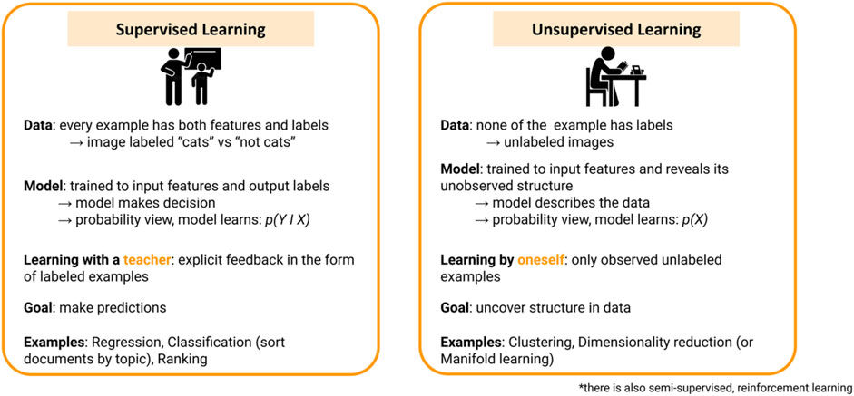
FIGURE 1. Summary of supervised learning and unsupervised learning approaches in machine learning applications.

During the advancement of a data science or ML project, it is essential to keep in mind that 1) the choice of the approach depends on the goal of the project, and 2) the goal(s) must be realistic and achievable. Moreover, the approach needs to be defined based on the structure and the properties of the data, which EDA helps the scientists understand. The problem to solve, and the available resources like data and domain knowledge will change the strategy to apply. Moreover, the science experts (in our case, mass spectrometry scientists) and data scientists need to work in close collaboration to correctly implement tools to achieve the main science goal(s), while respecting the project or mission constraints. In this work, we introduce a data science and ML pipeline for EDA of ocean worlds analog spectra, keeping in mind that similar techniques could be applied to other planetary instruments’ datasets.

2.2 Dataset description

Here we use laboratory analog datasets from Theiling (2021), as well as new data from ocean worlds seawater analogs and associated CO₂ that interacted with the seawater (Figure 2). These Enceladus- and Europa-relevant laboratory analog ocean world seawaters were previously analyzed to refine the current carbon and oxygen isotopic fractionation models for seawaters of various composition and pH (Theiling, 2021). In the present study, these data are used to understand the potential of CO₂ spectra to cluster by seawater environment. These seawaters are composed of varying ionic strengths and combinations of NaCl, MgCl₂, NaHCO₃, MgSO₄, and Na₂SO₄. CO₂ mixed with helium was injected in varying concentrations (0%, 0.3%, 1%, and 2%) to study the isotopic fractionation that occurs as each solution interacts with the CO₂. Each experiment was prepared and analyzed in triplicate. Experiments were equilibrated over varying times: 24, 48, 72, and 168 h. The standard equilibration time used after initial experimentation was 168 h. Isotope ratios (δ¹³C and δ¹⁸O) were analyzed using a trace gas analyzer (Gasbench II) coupled to an isotope ratio mass spectrometer (IRMS: Thermo Finnigan Delta V Advantage). Theiling (2021) demonstrates that the CO₂ concentration and pH affect the isotopic fractionation, which would affect isotope ratios measured during missions to Enceladus or Europa differently. In our present study, we use this CO₂ IRMS dataset to develop EDA methods, automated quality checks, processing, filtering, data analysis, and ML pipelines for predictions of seawater composition and identification of biosignatures. For EDA methods detailed in the current study, these proof-of-concept tools include basic data analysis methods and unsupervised ML techniques for detection and visualization of the data structure. Supervised ML techniques to learn underlying complex models and predict the composition of new, unseen data are the subject of future work. The driving goal of these algorithms is to develop an analytical software tool that could be used by mission scientists as a rapid data analysis method for returned data. A longer-term goal is to deploy further analytical ML tools onboard a spacecraft for automated real-time data analysis and decision-making.

FIGURE 2

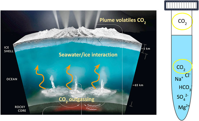
FIGURE 2. Schematic illustration of the internal structure and subsurface and surface interactions on Enceladus. CO₂ was measured in Enceladus’s plumes by Cassini, and is an expected product of rock-water interaction at the seafloor. This CO₂ would interact with the ocean before plume ejection. Laboratory experiments simulate the interaction of CO₂ with the seawater, and CO₂ is analyzed from the gaseous headspace. Figure modified from NASA/JPL-Caltech.

2.3 Preprocessing

Data from each experiment is composed of several measurements of volatiles over time in the headspace of a 12 mL vial containing 0.5 mL of an analog seawater. Experiments consist of repeated sampling using a double walled needle that exchanges sample gas with inert helium. These volatile measurements are then transferred to the IRMS through an 8-way valve, which effectively produces 10 discrete “sample” peaks (Figure 3). The data collection strategy was organized around several factors, with variations of each one as described in Table 1.

FIGURE 3

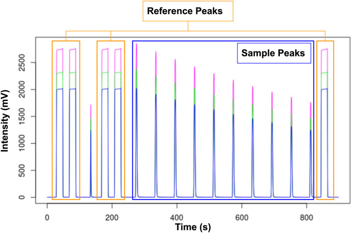
FIGURE 3. Typical trace gas analysis-IRMS example with 5 rectangular reference peaks (peaks 1, 2, 4, 5, 16 = orange rectangle), a valve flush peak to remove contamination (peak 3), and 10 sample peaks (blue rectangle). In our data processing, QA/QC, and ML analyses, we remove the first peak of the replicate sample peaks (peak 6) as it can potentially include residual gas from the previous sample.

TABLE 1

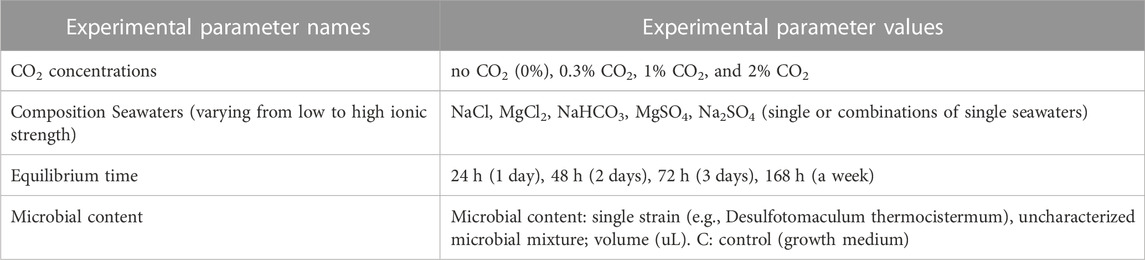
TABLE 1. Primary variables of the ocean worlds analog experiments data collection strategy. The composition of the seawaters varied by salt type, concentration, and whether the mixture was a single or multiple salt solution. The amount of initial CO2 interacting with these seawaters was varied, and whether seawaters were inoculated with single strains of microbes or complex microbial ecosystems. Equilibrium time was varied to compare data from disequilibrium conditions (<72 h) with those at equilibrium (≥168 h).

Data from each experiment is composed of raw chromatograms (x-axis: time (s), y-axis: voltage (mV)) and extracted data in tables representing spectral features such as isotope ratios (for CO₂), voltages (mV), and times (s), calculated features such as the fractionation values of these ratios (δ¹³C, δ¹⁸O), as well as experiment metadata such as CO₂ preparation concentrations, compound information, etc. Before training an ML algorithm to classify biotic versus abiotic compounds for instance, or to classify between the amount of injected CO₂, we need to understand the dataset and process it into high-quality input data for further data science and ML algorithm investigation/development. The first step consists of pre-processing the data from raw experimental data using automated quality analysis/quality control (QA/QC) designed using expert knowledge of our dataset, replicating the checks usually performed by science operations teams.

2.3.1 Raw data to quality checked data

Spectra from trace gas analysis using the Gasbench-IRMS are usually composed of 10 sample peaks, 5 reference peaks (reference gas measurements), and a valve flush peak to remove contamination from the previous sample (peak number 3) (Figure 3). The automated QA/QC pipeline outputs calibrated high-quality experimental data and removes poor-quality data while returning a summary of the analysis. This quality check pre-processing step prepares the dataset to be as robust as possible for follow-on statistical analyses and ML training. Some common data quality issues result from constricted flow and air contamination or sample transfer line clogging, which result in poor sample peak definition, additional peaks, inconsistency, or poorly defined or organized data. This pre-processing step is based on domain knowledge from IRMS experts who have developed a defined, agreed-upon set of rules and standards governing the experiment and dataset. For instance, a common quality check rule is that each spectrum has a defined number of peaks with a maximum of 18 peaks and a minimum of 14 peaks. For example, a simple quality check is for the expected number and retention time of peaks, since they are specified at the onset of the IRMS experiment and occur at programmed times. There are five reference peaks (peak numbers 1, 2, 4, 5, and 16), a flush peak (peak number 3), and ten sample peaks (peaks 7–15). Periodically during the high-throughput MS experiments, the IRMS samples known compounds (named “internal standards”) with known isotope fractionations to verify the quality of the run. In the creation of the studied dataset, we remove the flush peak (peak number 3 if present) as its main purpose is to remove contamination in the gas transfer system, and remove the first sample peak (peak number 6) as contamination from prior sample is sometimes present in the first subsample peak.

2.3.2 Data: from raw MS to time-averaged data

Mass spectrometers transfer samples in a gaseous form and ionize the sample gas to convert it into charged particles, and peripheral instruments are responsible for converting solid, liquid, or gas samples into a gas at some pressure or rate required by the instrument. The ionized gas is then accelerated toward detectors that determines the particles’ mass, which may be performed by measuring multiple times over a range of mass-to-charge (m/z) (e.g., ion trap mass spectrometry (ITMS)), or by interacting the charged particles with a magnet to deflect their path, and timing their transit to the detectors (e.g., time-of-flight (TOF) mass spectrometry). For SAM (Sample Analysis at Mars) instrument onboard Curiosity rover (Mahaffy et al., 2012), MOMA (Mars Organic Molecule Analyzer) that will be onboard the ExoMars mission (Goesmann et al., 2017), or EMILI (Europan Molecular Indicators of Life Investigation) for Europa exploration (Brinckerhoff et al., 2022), the samples studied are being ionized for a specific duration in a trap before being released to the instrument’s detector (ITMS). The detectors continuously make measurements over the duration of the experiment and the outcomes are mass spectra with a time dimension.

As detailed above, experiments (vial of seawater analog) are repeatedly sampled over a period of time, adding a time component to IRMS data. The detectors make repeated measurements over the duration of the experiment and the outcomes produce intensity versus time chromatograms. A simple reduction of these repeated measures is to compute a mean and standard deviation of IRMS-generated variables (e.g., peak intensity, area, isotope ratios, etc.) for EDA. This process generates a high-dimensional variable space of MS-derived features with physical meaning for EDA and ML methods. We use IRMS data as raw data and converted it into a time-averaged dataset in order to significantly reduce the dimensionality of the input data while preserving the relevant information. For the raw data, each experiment has 9 sample peaks, and the input csv file is composed of 3,474 rows. On the other hand, the averaged data inputs all the 9 scientific peaks and computes the average over the 9 peaks. Each experiment is now represented by a single point and the input csv file has 386 rows (3,474/9).

2.4 Exploratory data analysis (EDA)

After performing QA/QC checks, we perform Exploratory Data Analysis (EDA)—a critical process of performing initial investigations on data in order to discover patterns, find anomalies such as outliers, and test initial hypothesis and assumptions with some statistics and visual representations. EDA is a tool used to better understand the dataset and prepare it as well as possible for further ML algorithms implementation. Indeed, EDA is an initial and fundamental step to learn patterns from your data that could then be leveraged to create precision algorithms that focus on onboard capabilities to support science investigations.

2.4.1 Getting to know your data

Any computer science problem with data science and ML applications must start with steps to understand the data and gather as many insights as possible from it. The main goal of EDA is to make sense of the data before developing any algorithms with it. Initial investigations of the dimensionality of the data and the generation of summary statistics (supp table**) can give insights into data quality and the potential for outliers. Here, we describe an advanced EDA pipeline that yields more understanding into the nature of the data. The specific nature and properties of data, such as repeated measures, multicollinearities, and missing values, should inform the design of further data science and ML methods.

Initial basic steps start with loading the dataset, looking at the first few rows, getting the shape (e.g., the number of rows and columns) of the studied dataset, analyzing the variables stored in the columns and their corresponding data types, as well as finding whether some rows or columns contain null or missing values. A summary of statistics returns the count, mean, standard deviation, quantiles, minimum and maximum values. A quick look at this statistics summary gives a first idea of its quality and potential outliers in the dataset (Supplementary Table S1 in the annex).

2.4.2 Metadata analysis

It is necessary to understand whether the data contains multicollinearities between features that add redundancy and noise to the ML training process. A straightforward method for studying correlations in the dataset is to visualize the correlation matrix via a heatmap (Figure 4). Correlation scores close to 1 (represented in green) represent a positive correlation, while scores closer to −1 (represented in red) illustrate a negative correlation. During the features selection step, correlated variables are removed in order to reduce the dimension of the dataset while retaining the most information.

FIGURE 4

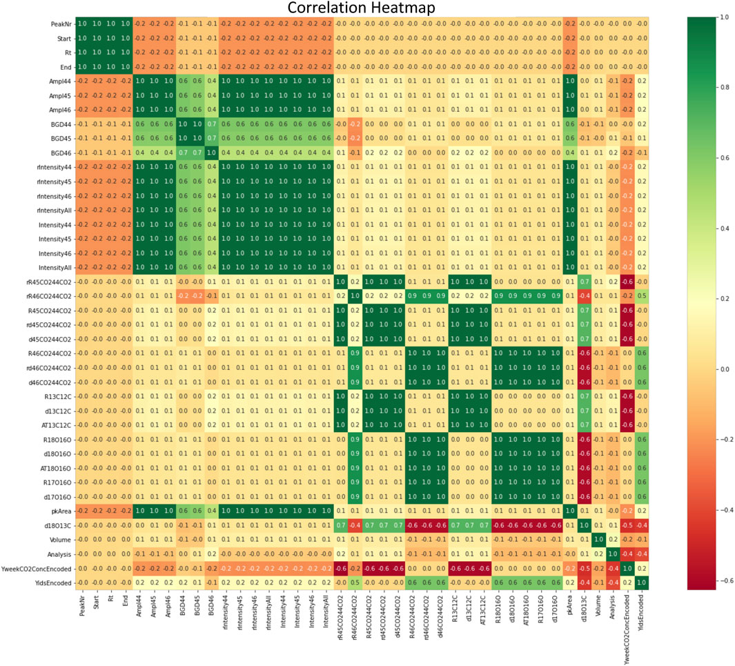
FIGURE 4. Correlation matrix (heatmap) of all 41 features from the MS instrument. This correlation matrix shows correlation coefficients between variables of the input dataset. Each cell represents the correlation between 2 variables. A correlation heatmap is used to summarize the data and is a diagnostic for advanced analyses such as machine learning.

In the correlation matrix of our studied dataset, we observe that “PeakNr”, “Start”, “Rt”, and “End” (described in the Supplementary Table S2) are highly correlated and effectively contain the same information (upper left corner of Figure 4). Indeed, these four features represent the same concept: the temporal dimension of each peak. On the other hand, we observe that “d18O13C” is negatively correlated (correlation value of −0.6) with the ratios of ⁴⁶CO₂ to ⁴⁴CO₂ (named “R46CO244CO2”, “rd46CO244CO2”, “d46CO244CO2” in the Supplementary Table S2). There are multiple perfect correlation blocks (dark green in Figure 4) that can be collapsed into one unit of analysis.

Boxplots and pairplots are other common types of plots useful to display the distribution of the studied data. Boxplots display the 5 main statistical values: minimum, maximum, median, first, and third quartiles. Such distribution graphs provide a first glimpse at potential outliers and enable us to look at the relationships between the variables in more detail than a correlation heat map. Pairplots represent pairwise relationships in the input dataset and help to understand the best set of features to explain relationships between two variables. They also help distinguish the most separated clusters of data, thus forming simple classification models. Pairplots from our example dataset (Figure 5) illustrate several important differences between “abiotic” samples (orange) and those inoculated with microbes “biotic” (green).” In these examples, the plots on a diagonal from the upper left to lower right illustrate distribution plots of each variable in the data output. As such, these plots demonstrate a strong differentiation of biotic and abiotic data in terms of R45CO244CO2 and d13C12C (δ¹³C), yet that distributions for R46CO244CO2 and d18O16O (the isotope ratio of oxygen, δ¹⁸O) are more similar for abiotic and biotic samples. This observation suggests that differences between abiotic and biotic samples may be best represented by changes in isotopologues of CO₂ (R45CO244CO2) and carbon isotope ratios (d13C12C, the isotope ratio of carbon, δ¹³C).

FIGURE 5

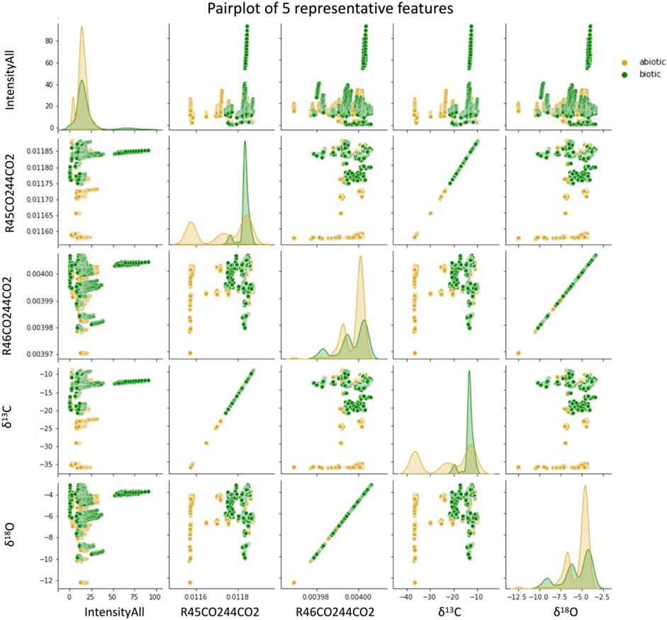
FIGURE 5. Pairplot of five representative input features of the studied dataset. The diagonal represents the distribution plot of each variable, and other plots represent each variable against the rest of the variables. Pairplots are powerful tool to quickly explore distributions and relationships in any dataset. For instance, here we can notice the linear relationship between R45CO244CO2 and δ¹³C, and between R46CO244CO2 and δ¹⁸O.

In contrast, each plot outside of this diagonal represents each variable against a different variable. For example, Figure 5 illustrates a linear relationship between δ¹⁸O (d18O16O) and R46CO244CO2. This is an expected result, as δ¹⁸O is linearly calculated based on the ratio of isotopologues with mass 46 and mass 44 (R46CO244CO2), and therefore is not expected to be a distinct measurement. Therefore, distribution plots such as pairplots (and boxplots) can be a rapid and useful tool to understand which variables are important for specific types of follow-on analysis, including machine learning. These initial EDA techniques are useful in understanding the nuances of the dataset and further enable an informed approach to development of algorithms for prediction or classification.

2.5 Unsupervised learning

As mentioned above, unsupervised learning algorithms are used to explore and analyze the structure of the data to identify patterns and similarities (clustering) or to simplify the dataset (dimensionality reduction) without being influenced by an assigned class label. Unsupervised learning algorithms are applicable when the phenomenon driving the data is unknown. Rather than making predictions about unknown data, the unsupervised algorithm provides insights on the relationships within the data, allowing us to see patterns otherwise not recognizable by human investigators. A first step is typically to use dimensionality reduction algorithms to represent the high-dimensional input data into a low dimensional space that retains the inter-variable relationships of the original data. This first step aims at getting a better understanding and interpretation of the data, and is often used as a precursor step to use clustering techniques to find unbiased patterns and similarities that group data into clusters of similar and dissimilar information.

2.5.1 Dimensionality reduction (PCA, t-SNE, UMAP)

Dimensionality reduction is the process of transforming a dataset with a large number of features to a representation with much fewer features, often for visualization purposes. The two main categories are linear methods and nonlinear methods. Principal Component Analysis (PCA) (Jolliffe and Cadima, 2016) is one of the most common linear dimensionality reduction techniques. PCA is a rotation of a multivariate dataset with new axes or effective variables called “principal components.” Each new component is a linear combination of the original variables, and they are ordered by their variance. The PCA method can represent the multidimensional dataset in a lower dimension by projecting the samples in a space defined by the first few principal components. PCA helps one visualize important correlation structure, that is, hidden in the higher dimensional representation. In contrast, T-distributed stochastic neighbor embedding (t-SNE) (Van der Maaten and Hinton, 2008) is a nonlinear dimensionality reduction algorithm that finds clusters in data, keeping similar instances close to each other and dissimilar instances apart. The algorithm creates a high dimensional graph and reconstructs it in a lower dimensional space point by point while retaining the structure. Another common nonlinear dimensionality reduction method is Uniform Manifold Approximation and Projection (UMAP) (McInnes et al., 2018), which has demonstrated strong effectiveness for visualizing clusters of data points and their relative proximity, and often preserves the global structure of the data more accurately than tSNE; the main difference is that UMAP compresses the graph reconstructed in a lower dimension.

Figure 6 illustrates these three techniques for the ocean worlds dataset as an exploratory technique for showing inherent similarities and patterns in the experimental data. Such visualizations can use color in various ways to understand how data are organized. The examples here are assigned different colors for each unique chemical composition [salt(s) and ionic strength], which is coded as their “Identifier1” in the instrument software. Figure 6 demonstrates that t-SNE and UMAP methods (Figures 6B, C) generate more distinctive groupings of samples over PCA (Figure 6A), and are better able to separate the data based on their chemical compositions and on their CO₂ concentration. Emergent arcs and lines for the same composition (e.g., an arc of MgSO4 L) in t-SNE and UMAP (Figures 6B, C) are explained by the subsampling of experiments; therefore, arcs and lines demonstrate grouping relevant to time in the spectra. Identifying the cause of emergent patterns from these dimensionality reduction techniques can be used as a pre-processing step to identify common features in the data, which enables selection of the best techniques for future ML work (e.g., dataset preparation and labeling, clustering algorithms, feature selection). In this case, t-SNE and UMAP demonstrated a potential training bias related to the subsampling technique and informed future dataset preparation.

FIGURE 6

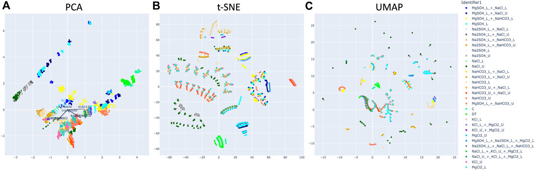
FIGURE 6. Comparison of 3 dimensionality reduction techniques, (A) PCA, (B) t-SNE, (C) UMAP on 15 selected features on the input dataset. The color legend represents the salt compositions of the seawaters (“Identifier1”). L/U indicate a lower/higher concentration of the salt. t-SNE and UMAP methods perform a more definite grouping of samples. Black vectors on subplot (A) (PCA) show the contribution of each feature for the PCA decomposition (discussed further in Figure 12).

2.5.2 Clustering algorithms

Data mining techniques have greatly supported the discovery of significant patterns in mass spectrometry data, particularly in proteomics and metabolomics (e.g., Thomas et al., 2006; Swan et al., 2013; Wang et al., 2020; Suvarna et al., 2021; Neely and Palmblad, 2022). Such studies are enabled by the availability of datasets. Developing these tools for exploration of planetary bodies, such as ocean worlds, is challenging due to the paucity of available data–either from the targets directly, or from modeling and laboratory studies; thus, few to no predictive labels are available for training. As a result, we use clustering techniques to support the discovery of inherent patterns in spectra due to chemical or physical properties. The task of clustering consists of organizing sets of data whose classification is unknown (no available labels) into meaningful groups (“clusters”) based on inherent relationships discovered from the input data. Data in the same clusters are more similar to each other than to objects in other clusters. Clustering results and assessments are then used for patterns evaluation (e.g., discriminatory patterns) and as a filtering tool.

Several clustering algorithms exist and can be grouped in 3 main families: partitional clustering, hierarchical clustering, and density-based clustering. In partitional clustering, the data is divided into non-overlapping groups, meaning that each object is assigned to a single cluster (Gandhi and Srivastava, 2014; Kutbay, 2018). The KMeans algorithm (Kanungo et al., 2002) is a type of partitional clustering. One drawback of this approach is the need to specify the number of clusters, necessitating some interpretation of the data; we consider this approach to be ‘semi-automated.’ As an example, Figure 7 shows a UMAP representation using KMeans algorithm to assign samples to 8 clusters that each represent the primary salts used in the laboratory experiments. Clusters are generally distinct for each assigned cluster, suggesting that salt composition (color) has a significant effect on clustering. However, Figure 7 demonstrates that, e.g., NaHCO3-based seawaters are partitioned among several assigned clusters (red, green, cyan, lime), which may be promoted by differing ionic strength, the concentration of CO₂, or combinations with other salts (multiple salt solutions described in Theiling (2021)). Therefore, partitional clustering can be used as an exploratory tool to determine which features of a dataset affect the organization.

FIGURE 7

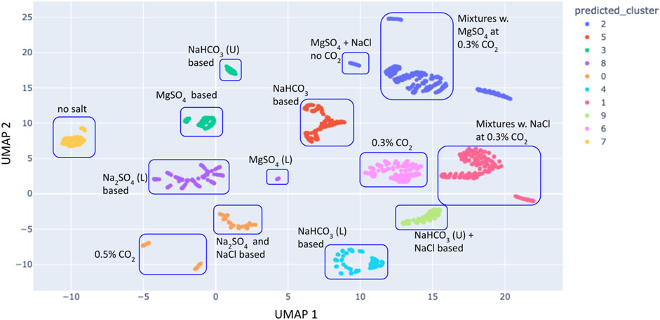
FIGURE 7. K-Means clustering of a two components UMAP representation of the repeated measures dataset (data not averaged) and using n_clusters = 8 clusters (representing the main salts used in the experiments). The plot is annotated with the main salt present in each cluster of points.

The second family of clustering is hierarchical, whereby the algorithm builds a hierarchy to determine cluster assignments (Cohen-Addad et al., 2017). These can be further divided into two types of approaches. First is a top-down approach called “divisive clustering”, in which all the points are initially part of a single cluster, and points are iteratively split into least similar clusters until each cluster is composed of a single point. The second is a bottom-up approach is called “agglomerative clustering”, whereby each point starts as individual cluster, and the algorithm iteratively merges the most similar two points until all points are part of a unique cluster.

The last common technique is density-based clustering, which builds clusters based on the density of data points in a region (Ester et al., 1996; Sander et al., 1998). Clusters are drawn where high-densities of data points separated by low-density regions. This method does not require the user to specify the number of clusters, but instead uses a distance-based metric as a tunable threshold.

As noted above, some of these clustering algorithms require the user to input the number of clusters. In an unsupervised, data-driven approach, users either do not know the number of clusters that will best partition their data, or do not want to introduce bias. Several methods exist to evaluate the best number of clusters (Lamirel et al., 2016), which we illustrate in Figure 8. The Elbow method is the most popular method, and runs the clustering algorithm several times with different values of k (number of clusters) (Marutho et al., 2018). The user then plots the sum of squared errors (SSE) vs. k, and finds the optimal number of clusters in the elbow of the curve (when the change in SSE first starts to diminish). Another common method is the Silhouette index. The silhouette value measures how similar a point is to its own cluster (cohesion) compared to other clusters (separation). Values range from −1 (clusters being assigned the wrong way) to 1 (clusters are well apart from each other and clearly distinguished). The higher the silhouette value, the better the model (Rousseeuw, 1987; Dudek, 2020). Another method is the Calinski-Harabasz (CH) index. This index measures the compactness and separation between clusters, interpreted such that good clusters are themselves very compact and well-spaced from each other. Higher the CH index, the better the model (Calinski and Harabasz, 1974). Similarly as the CH index, the Davies-Boulding (DB) index measures the compactness and separation between clusters. The lower the DB index, the better the model (Davies and Bouldin, 1979). Finally, one may use a Dendrogram; A tree-structured graph used to visualize the result of a hierarchical clustering calculation. The dendrogram first starts by considering each point as a single cluster and joins points to clusters in a hierarchical manner based on their distance (the user specifies the distance metric to use; here we use Euclidean distance). The heights of the joins between clusters represents the distance between those clusters (Forina et al., 2002). We posit that ultimately the choice for the number of clusters to use should be guided by both clustering evaluation metrics described above (data-driven) and domain knowledge (knowledge-driven).

FIGURE 8

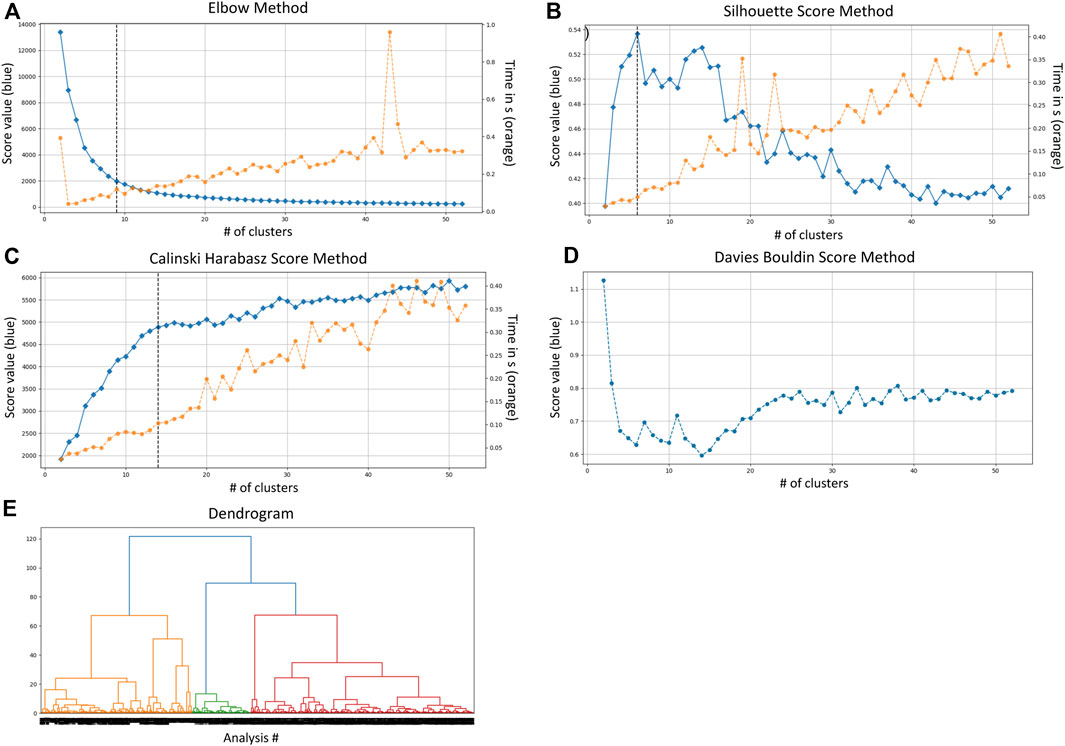
FIGURE 8. Results of 5 methods aiming at finding the best number of clusters for the dataset The left vertical axes represent the value of the specific score being measured. The right vertical axes [subplots (A–C)] represent the computation time (in seconds). The vertical line is the result representing the optimal number of clusters for each technique: (A) elbow method, 9 clusters; (B) silhouette score, 6 clusters; (C) Calinski-Harabasz method, 14 clusters; (D) Davies Bouldin score, 14 clusters; (E) dendrogram, 6 clusters (to define for the dendrogram).

3 Experimental pipeline and implementation

3.1 EDA for quality checks

We use EDA techniques such as basic statistics (average, quartiles, minimum, and maximum values) and visualization plots like boxplots and pairplots in an iterative process for the verification of the QA/QC steps. After each implementation of a new QC, pairplots and boxplots are generated to verify the presence of potential outliers representing poor quality laboratory data that should be filtered out, which are cross-checked with more laborious QA/QC procedures typical for evaluating similar data types, including visual inspection of chromatograms and filtering, sorting, and calibration procedures performed in spreadsheets. Unlike analysis of natural samples, in which the purpose is to characterize unknown materials, the purpose of the ocean worlds experimental dataset we use is to understand similarities and differences in output under highly-constrained conditions. Therefore, we must understand how variable data quality might interfere with data from the experimental conditions (i.e., reduce the probability of false positives/negatives, aid in instrument diagnosis).

Figure 9 illustrates five features [“PeakNr” (peak number), “Rt” (retention time), d13C12C, d18O16O, and Ampl44] from unfiltered data compared to those that underwent a first quality check implementation for the 5 reference peaks. We first focus on the 5 reference peaks as they offer clear readability of the outliers. We quickly observe that the number of peaks is reduced from 32 to 16 (last reference peak is peak #16), and the values range of d13C12C and d18O16O is rescaled. This suggests that our EDA process could assist in identifying poor quality data, and also demonstrates the improvement of the dataset using established QC checks on overall data. This is also important to note because a user could use additional EDA or ML on raw, QA/QC checked, or QA/QC checked and calibrated data. These pairplots therefore demonstrate that additional processing of data will improve results. Thus, EDA techniques could be used on raw data to understand structure and potential QA/QC flags, and then again on more processed data to evaluate scientific questions.

FIGURE 9

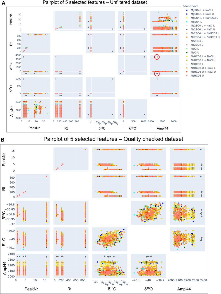
FIGURE 9. Comparison of pairplots for the unfiltered dataset before any quality checks [subplot (A)] and post quality checks [subplot (B)]. For clear readability in this example, we only represent the 5 reference peaks for 5 features. The unfiltered data [plot (A)] shows PeakNr values from 0 to 32, while the quality checked one [plot (B)] shows the right number of 5 reference peaks (peaks 1, 2, 4, 5, and 16). The features δ¹³C, δ¹⁸O, and Ampl44 unrealistic values (for instance δ¹³C from −50–3500) on the unfiltered dataset due to the presence of outliers’ values (circled in red on the δ¹³C vs. Ampl44 subplot), while being corrected in the post quality checked data.

3.2 Choice of features of interest

Correlation matrices depict the correlation between all possible pairs of values in the table. This is a powerful tool to summarize datasets with many features and to identify patterns in the given data. In Figure 10, we represent a correlation matrix for 3 different sets of features: 1) all the 41 features, 2) a limited set of 25 features, and 3) an even more limited set of 14 features. Limited features in Figure 4B are selected based on characteristics typically used to evaluate chromatograms, and these features were further down-selected in 4c based on correlations demonstrated in 4b. The choice of which features to remove is based on the high positive correlations represented by the green squares and a correlation value equal to 1. For instance, for a given isotope with mass X, “rIntensityX”, “IntensityX”, and “AmplX” contain the same information and are considered redundant in terms of their information content, although their absolute values may be unique. Removing highly correlated variables is needed to prepare the dataset for ML, streamlining processing and improving interpretability of the model.

FIGURE 10

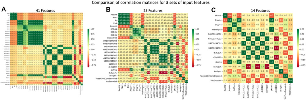
FIGURE 10. Comparison of correlation matrices for 3 different input sets: all 41 features (A), a limited set of 25 features (B), and a smaller set of 14 features (C). Redundancies (green) are reduced by down-selecting features.

Moreover, down-selecting features improves dimensionality reduction techniques. In the case of applying PCA (i.e., a dimensionality reduction tool that helps identify patterns in the dataset based on the correlations between features), removing highly correlated features enhances the output reduced set. The mathematical process of PCA aims at finding the directions of maximum variance in the high-dimensional space and at projecting it a lower dimension space. By keeping strongly correlated features before performing PCA, the contribution of their common underlying factor increases and can have substantial effect on PCA results. Even if PCA is not a feature selection method, it is common to consider the ranking of the features in the explained variance and only retain the most important features that explain most of the variance.

We analyze the role of each feature using 3 different sets of input features for PCA application (Figure 11): 10 features (Figures 11A, D), 5 features (Figures 11B, E), and 2 features (Figures 11C, F). When plotting the PCA results we add vectors representing the direction, orientation, and amplitude of each input feature. Figure 12 illustrates the high correlation between some input features such as Start/End (representing the timing of the sample or standard peak), d13C12C/d18O16O (representing the ratio of CO₂ isotopologues measured in the experiment). Using these PCA results, we are then able to reduce the input features to best represent the dataset while preserving the most information.

FIGURE 11

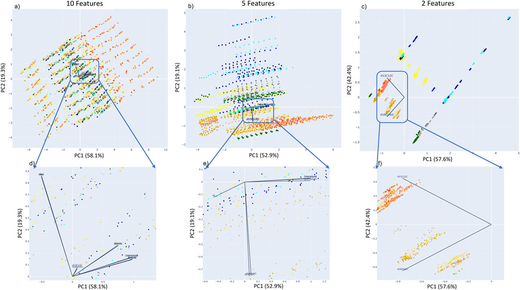
FIGURE 11. Comparison of 3 PCA plots for different input features set: (A) the 10 main features, (B) 5 limited features, and (C) only the two isotopic measurements (δ¹³C and δ¹⁸O). Plots (D), (E), and (F) are a zoom on the vectors representing the role of each feature for each principal component.

FIGURE 12

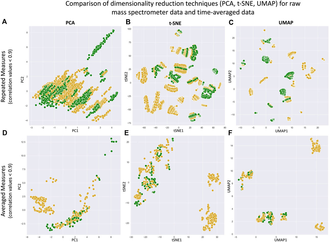
FIGURE 12. Comparison of 2-components PCA (subplots a and d), t-SNE (subplots b and e), and UMAP (subplots c and f) algorithms on raw mass spectrometry data [with multiple observations for each experiment, subplots (A–C)] and averaged MS features data [one observation per experiment, subplots (D–F)]. The color legend represents biotic (green) vs. abiotic (gold). The application of these dimensionality reduction algorithms on the averaged dataset offers fewer initial clusters representing abiotic versus biotic samples.

3.3 Comparison of repeated measures data and averaged data

Similar to PCA, t-SNE and UMAP representations in Figure 7, the linear patterns emerging in Figures 12A–C are due to repeated measures of each sample peak. Therefore, to remove the bias in continued data science and ML techniques, we average the repeated measures, resulting in more clear cluster structure (Figures 12D–F). In the raw data, each experiment consists of CO₂ equilibrated with an ocean world analog seawater, and repeated sampling by the IRMS results in 9 sample peaks used for further analysis (Figure 3). As a simple first transformation, we create a separate dataset in which the 9 sample peak values are averaged into a single value, and all potential features including a time component (e.g., Rt, Start, End, etc.) are removed. This averaging of the repeated measures results in a dataset, that is, more conducive to further analysis and ML.

We analyze the differences of the repeated measures dataset (only features with correlation lower than 0.9 have been used in these representations) and the time-averaged dataset. We note that PCA, t-SNE and UMAP algorithms used as dimensionality reduction techniques are able to simplify the clusters when using the mean-reduced data versus the repeated-measures data. By limiting the number of repeated measures per experiment (by averaging) and by limiting the numbers of features (only the ones with correlation values <0.9), these basic dimensionality reduction algorithms demonstrate they are better at clustering than the raw data.

4 Discussion and lessons learned

Our work is already yielding several lessons learned and directions for the next steps to develop onboard science data analysis for future mature missions.

4.1 Implementation, limitations, and challenges

Solar system missions not only present operational challenges but also technological ones. Indeed, the harsh environment the spacecraft are exposed to, such as extreme temperature gradients and radiation, constantly damage the electronics components, limiting the diversity of hardware usable on spacecraft. An additional challenge therefore is accommodating the computational requirements for onboard data science and ML processing. These computing requirements pose a difficult problem for the application to space missions, which are extremely limited in power consumption, communication bandwidth, and hardware equipment. The majority of NASA missions require “Radiation Hardened” (RH) electronics, including everything from power supplies to general purpose central processing units (CPUs), or requirements for certain electronics to be house in a radiation hardened vault. These requirements limit the available power and data volume, creating a widespread need for technological development in RH processing capability. As an example, the Curiosity rover, the Perseverance rover, and the Mars Reconnaissance Orbiter (MRO) are all equipped with the same RH CPU (BAR Systems RAD750 processor) that was developed in the 1990s. The demonstrated flight heritage (TRL 9) and reliability of the RAD 750 makes it a standard in space missions, despite many generations behind the state-of-the-art in processors. The emergence of FPGAs (Field-Programmable Gate Array, i.e., integrated circuit designed to be configured by a customer) with DSP (Digital Signal Processors) or simple integrated neural processors shows promise that sufficient AI and ML application hardware will soon be developed for space flight applications. However, the mission design requires an exploration of tradeoffs between runtime and accuracy to offer tools that answer science objectives while respecting operational constraints. ML evolves very quickly and the latest sophisticated models cannot fit in the severe resource constraints. To date, computer science tools that have been deployed in space have low computational demands. One of the next steps is to monitor the power, memory, and computation time for the methods mentioned in this paper. During the development of these algorithms, we kept in mind the needs of performance and resource-optimization due to high limitations for planetary missions.

Moreover, ML applications require large amounts of data in order to properly train and tune the developed algorithms. In this work, we use data collected in a laboratory over 2 years. The total dataset was composed of 1,086 input spectra, reduced to 587 spectra after the quality check process. While more data are being collected in the laboratory, this process can take many years; therefore. Data generation techniques to enhance the input dataset, such as synthetic data creation or data augmentation methods (Maharana et al., 2022; Mikolajczyk et al., 2018) could be investigated in future research. This work is a proof-of-concept demonstrating a powerful data science pipeline that can support scientific research in a multitude of ways—from implementing automated checks on data quality and reproducibility, to understanding emergent patterns in datasets that may be outside typical uses of a dataset. By introducing these procedures here, we endeavor to inspire development of science- and mission-enhancing tools, including deployment of onboard analysis. We acknowledge, however, that data from flight instruments are often significantly different from commercial instruments, therefore models developed on commercial instrument data will need to be updated to be implemented on actual flight instrument data.

4.2 Data collection strategy

The investigation and development of intelligent algorithms to support space mission operations, using data science, basic thresholds methods, AI, or ML require the mission and instrument design to accommodate this innovative implementation. One of the key points is the creation of the dataset used to train and test the algorithms. The dataset must be well defined from the beginning of the mission concept in order to support effective and accurate algorithms to answer the specific requirements of the mission (operational, scientific, and engineering). Instrument scientists must establish precise goals and a coherent and clear dataset strategy creation. For this research, data scientists had to preprocess the dataset several times to remove unsuitable data and to reformat data collected in inconsistent ways by multiple users. Therefore, thinking about ML or data science applications from an early stage in the mission design will drive the data collection plan and greatly enhance the possibilities of data-driven algorithmic investigations.

4.3 Trust readiness level

The increasing presence of AI and ML is also accompanied with rising concerns, especially in domains like space exploration. The deployment of onboard intelligence techniques is still avant-garde and consequently high-risk. Every new technology or capability confronts a trade-off between the new benefits added to the instrument and deliverables, and the potential additional risks from its implementation. ML techniques must be fully tested and proven in order to demonstrate ML reliability. Moreover, it is worth mentioning that traditional algorithmic approaches such as threshold-based algorithms should be first considered if they enable the same science benefits while being more easily implementable onboard a mission than more opaque data science techniques. Algorithms must be designed in order to provide interpretability and limit this “black-box” effect.

Another important characteristic in the design and conception of AI and ML methods is the choice of the performance metrics based on the interest of the stakeholders. In our research, ML metrics such as accuracy, recall, and precision are being used in combination with scientists’ interpretations. The communication between the fields of data science and mass spectrometry is crucial to fully understand the needs of the science team as well as the limitations they face, and will be instrumental in promoting more widespread use and development of these tools among the scientific community.

Slingerlan and Perry (2022) provides a framework for developing trust in AI as further applications will require careful considerations of the training and the deployability of software and hardware in more realistic and therefore constrained environments. Recent research considered the development of a “Trust Readiness Level”, similar to the “Technology Readiness Level” (TRL) used in the spaceflight engineering field for hardware ability evaluation (Da Poian et al., 2022). Our research aims at designing a scale system to assess the maturity level of the technology using AI and ML tools. Similarly to the engineering scale, this trusting system will follow a progressing path that tests these methods on laboratory data in normal conditions, and then under more realistic flight mission conditions and constraints before being actually used onboard a mission. This Trust Readiness Level scale will not only be dependent of the target of interest but also on the types of instruments. Because mass spectrometers going to Mars will not have the same constraints and requirements as the ones going further out in our Solar System (to Titan onboard Dragonfly, to Europa onboard the Europa Clipper mission), this trust readiness level scale will be dependent of the target of interest for the mission. It will also be dependent on the type of instruments under study while studying the same target of interest, as for instance mass spectrometers and magnetometers will not hold the same requirements and constraints and will though have different trust demands. Developing this trust readiness level will require a systematic methodology, consistency, and adjustment on a case-by-case basis.

5 Conclusion and future work

The upcoming decade will launch another revolution in planetary exploration with the fascinating advances in flight science instruments. International space agencies are developing more mature and sophisticated missions to explore environments in our Solar System that were previously considered too risky; with this we will better understand planetary processes and potential evidence of life beyond Earth. Beyond the continuous improvements of planetary instruments, it is now imperative to develop a modern framework to consider data from these missions, not only to enhance science return, but also to give autonomy to these visionary missions. We used ocean worlds laboratory analogs to develop an initial data processing pipeline as a proof-of-concept to evaluate whether volatile CO₂ emanating from Europa or Enceladus could contain any information related to the surface and subsurface ocean composition; these ML algorithms are in refinement. However, our discussion here of EDA techniques could serve as a guide for other researchers considering ways to enhance data return from missions or laboratory experiments. Such data science approaches and future ML algorithms are developed to advance analytical software tools that could be used by mission scientists as methods for rapid data analysis. Science autonomy enabled by tools like data science and ML will ultimately empower the reach of future mission targets such as icy ocean worlds or targets further away out of our Solar System, ensuring future outstanding scientific discoveries.

Data availability statement

The original contributions presented in the study are included in the article/Supplementary Materials, further inquiries can be directed to the corresponding author.

Author contributions

VD wrote the first draft of the manuscript. All authors contributed to the article and approved the submitted version.

Funding

VD was supported by a FLaRe funding at the NASA Goddard Space Flight Center, administered by Microtel LLC. BPT was supported by FLaRe funding at the NASA Goddard Space Flight Center. Support for this research was provided by NASA’s Planetary Science Division Research Program, through the Internal Scientist Funding Model (ISFM) Fundamental Laboratory Research (FLaRe) work package at NASA Goddard Space Flight Center in the Planetary Environment Laboratory (Code 699).

Acknowledgments

The authors would like to acknowledge Sascha Kempf, an reviewer, and the editors for providing feedback which greatly helped in improving the clarity of the manuscript.

Conflict of interest

Author VD was employed by the company Microtel LLC.

The remaining authors declare that the research was conducted in the absence of any commercial or financial relationships that could be construed as a potential conflict of interest.

Publisher’s note

All claims expressed in this article are solely those of the authors and do not necessarily represent those of their affiliated organizations, or those of the publisher, the editors and the reviewers. Any product that may be evaluated in this article, or claim that may be made by its manufacturer, is not guaranteed or endorsed by the publisher.

Supplementary Material

The Supplementary Material for this article can be found online at: https://www.frontiersin.org/articles/10.3389/fspas.2023.1134141/full#supplementary-material

References

Andres, C., Fukunaga, A., Biesiadecki, J., Lynn, N., Whelley, P., Greeley, R., et al. (2008). Automatic detection of dust devils and clouds on Mars. Mach. Vis. Appl. 19, 467–482. doi:10.1007/s00138-007-0081-3

CrossRef Full Text | Google Scholar

Brinckerhoff, W., Willis, P., Ricco, A. O., Kaplan, D. A., Danell, R. M., Grubisic, A., et al. (2022). Europan molecular indicators of life investigation (EMILI) for a future Europa lander mission. Front. Space Technol. 2. doi:10.3389/frspt.2021.760927

CrossRef Full Text | Google Scholar

Brockwell, T., Meech, K., Keith, P. S., Waite, J. H., Miller, G., Roberts, J., et al. (2016). “The mass spectrometer for planetary exploration (MASPEX),” in IEEE aerospace conference 2016. doi:10.1109/AERO.2016.7500777

CrossRef Full Text | Google Scholar

Calinski, T., and Harabasz, J. (1974). A dendrite method for cluster analysis: Communications in statistics. Theory Methods 3, 1–27. doi:10.1080/03610927408827101

CrossRef Full Text | Google Scholar

Chien, S., Bue, B., Castillo-Rogez, J., Gharibian, D., Knight, R., Schaffer, S., et al. (2014). Agile science: Using onboard autonomy for primitive bodies and deep space exploration. Proc. Intl. Symposium Artif. Intell. Robotics, Automation Space. doi:10.2514/6.2014-1888

CrossRef Full Text | Google Scholar

Chou, L., Paul, M., Trainer, M., Eigenbrode, J., Arevalo, R., Brinckerhoff, W., et al. (2021). Planetary mass spectrometry for agnostic life detection in the solar system. Front. Astronomy Space Sci. 8. doi:10.3389/fspas.2021.755100

CrossRef Full Text | Google Scholar

Cohen-Addad, V., Kanade, V., Mallmann-Trenn, F., and Mathieu, C. (2017). Hierarchical clustering: Objective functions and algorithms. Arxiv. doi:10.48550/arXiv.1704.02147

CrossRef Full Text | Google Scholar

Da Poian, V., Lyness, E., Ryan, D., Xiang, L., Theiling, B., Trainer, M., et al. (2022). Science autonomy and space science: Application to the ExoMars mission. Front. Astronomy Space Sci. 9. doi:10.3389/fspas.2022.848669

CrossRef Full Text | Google Scholar

Davies, D., and Don, B. (1979). A cluster separation measure. IEEE Trans. PAMI- 1, 224–227. doi:10.1109/TPAMI.1979.4766909

PubMed Abstract | CrossRef Full Text | Google Scholar

Dudek, A. (2020). “Silhouette index as clustering evaluation tool,” in Classification and data analysis. SKAD 2019. Studies in classification, data analysis, and knowledge organization. Editors K. Jajuga, J. Batóg, and M. Walesiak (Cham: Springer). doi:10.1007/978-3-030-52348-0_2

CrossRef Full Text | Google Scholar

Ester, M., Kriegel, H.-P., Sander, J., and Xu, X. (1996). “A density-based algorithm for discovering clusters in large spatial databases with noise,” in The second international conference on knowledge discovery and data mining. AAAI Press. Kdd 96.

Google Scholar

Forina, M., Armanino, C., and Raggio, V. (2002). Clustering with dendrograms on interpretation variables. Anal. Chim. Acta 454 (1), 13–19. ISSN 0003-2670. doi:10.1016/S0003-2670(01)01517-3

CrossRef Full Text | Google Scholar

Francis, R., Estlin, T., Gaines, D., Bornstein, B., Schaffer, S., Verma, V. I., et al. (2015). “AEGIS autonomous targeting for the curiosity rover's ChemCam instrument,” in IEEE applied imagery pattern recognition workshop (AIPR) (Washington, DC, USA: IEEE). doi:10.1109/AIPR.2015.7444544

CrossRef Full Text | Google Scholar

Francis, R., Estlin, T., Gary, D., Johnstone, S., Gaines, D., Verma, V.i, et al. (2017). AEGIS autonomous targeting for ChemCam on mars science laboratory: Deployment and results of initial science team use. Sci. Robot. 2. doi:10.1126/scirobotics.aan4582

PubMed Abstract | CrossRef Full Text | Google Scholar

Gandhi, G., and Srivastava, R. (2014). Review paper: A comparative study on partitioning techniques of clustering algorithms. Int. J. Comput. Appl. 87, 10–13. doi:10.5120/15235-3770

CrossRef Full Text | Google Scholar

Goesmann, F., Brinckerhoff, W., Raulin, F., Goetz, W., Ryan, D., Getty, S. E., et al. (2017). The mars organic molecule analyzer (MOMA) instrument: Characterization of organic material in martian sediments. Astrobiology 17, 655–685. doi:10.1089/ast.2016.1551

PubMed Abstract | CrossRef Full Text | Google Scholar

Jolliffe, I. T., and Cadima, J. (2016). Principal component analysis: A review and recent developments. Philos. Trans. A Math. Phys. Eng. Sci. 374, 20150202. doi:10.1098/rsta.2015.0202

PubMed Abstract | CrossRef Full Text | Google Scholar

Kanungo, T., Mount, D., Nathan, N., Piatko, C., Silverman, R., and Wu, A. (2002). An efficient k-means clustering algorithm: Analysis and implementation. IEEE Trans. Pattern Analysis Mach. Intell. 24 (7), 881–892. doi:10.1109/TPAMI.2002.1017616

CrossRef Full Text | Google Scholar

Kutbay, U. (2018). Partitional clustering. Recent applications in data clustering. doi:10.5772/intechopen.75836

CrossRef Full Text | Google Scholar

Lamirel, J.-C., Dugué, N., and Pascal, C. (2016). New efficient clustering quality indexes. Conference: International joint conference on neural networks. doi:10.1109/IJCNN.2016.7727669

CrossRef Full Text | Google Scholar

Mahaffy, P. (1999). “Mass spectrometers developed for planetary missions,” in Laboratory astrophysics and space research. Editors P. Ehrenfreund, C. Krafft, H. Kochan, and V. Pirronello (Dordrecht: Springer), 236. Astrophysics and Space Science Library. doi:10.1007/978-94-011-4728-6_13

CrossRef Full Text | Google Scholar

Mahaffy, P., Webster, C., Cabane, M., Conrad, P. G., Coll, P., Atreya, S. K., et al. (2012). The sample analysis at mars investigation and instrument suite. Space Sci. Rev. 170, 401–478. doi:10.1007/s11214-012-9879-z

CrossRef Full Text | Google Scholar

Maharana, K., Mondal, S., and Nemade, B. (2022). A review: Data pre-processing and data augmentation techniques. Glob. Transitions Proc. 3 (1), 91–99. ISSN 2666-285X. doi:10.1016/j.gltp.2022.04.020

CrossRef Full Text | Google Scholar

Marutho, D. A., Handaka, S. H., Wijaya, E., and Muljono, (2018). “The determination of cluster number at k-mean using elbow method and purity evaluation on headline news,” in 2018 international seminar on application for technology of information and communication. doi:10.1109/ISEMANTIC.2018.8549751

CrossRef Full Text | Google Scholar

Mauceri, S., Lee, J., Wronkiewicz, M., Mandrake, L., Doran, G., Lightholder, J., et al. (2022). Autonomous CE mass-spectra examination for the ocean worlds life surveyor. Earth Space Sci. 9, e2022EA002247. doi:10.1029/2022EA002247

PubMed Abstract | CrossRef Full Text | Google Scholar

McInnes, L., Healy, J., Saul, N., and Gorbberger, L. (2018). Umap: Uniform manifold approximation and projection for dimension reduction. Arxiv. doi:10.48550/arXiv.1802.03426

CrossRef Full Text | Google Scholar

Mikołajczyk, A., and Grochowski, M. (2018). “Data augmentation for improving deep learning in image classification problem,” in 2018 international interdisciplinary PhD workshop (IIPhDW). doi:10.1109/IIPHDW.2018.8388338

CrossRef Full Text | Google Scholar

Neely, B., and Palmblad, M. (2022). Machine learning in proteomics and metabolomics. J. Proteome Res. 21, 2553–2554. doi:10.1021/acs.jproteome.2c00566

PubMed Abstract | CrossRef Full Text | Google Scholar

Neveu, M., Hays, L., Voytek, M., New, M. H., and Schulte, M. D. (2018). The ladder of life detection. Astrobiology 18, 1375–1402. doi:10.1089/ast.2017.1773

PubMed Abstract | CrossRef Full Text | Google Scholar

Parvandeh, S., Yeh, H.-W., Paulus, M., and McKinney, B. (2020). Consensus features nested cross-validation. Bioinformatics 36, 3093–3098. doi:10.1093/bioinformatics/btaa046

PubMed Abstract | CrossRef Full Text | Google Scholar

Rousseeuw, P. (1987). Silhouettes: A graphical aid to the interpretation and validation of cluster analysis. J. Comput. Appl. Math. 20, 53–65. ISSN 0377-0427. doi:10.1016/0377-0427(87)90125-7

CrossRef Full Text | Google Scholar

Sander, J., Ester, M., Kriegel, H.-P., and Xu, X. (1998). Density-Based clustering in spatial databases: The algorithm GDBSCAN and its applications. Data Min. Knowl. Discov. 2, 169–194. doi:10.1023/A:1009745219419

CrossRef Full Text | Google Scholar

Slingerland, P., Perry, L. N., Kaufman, J., Bycroft, B., Linstead, E., Mandrake, L., et al. (2022). Adapting a trusted AI framework to space mission autonomy. IEEE 2022. doi:10.1109/AERO53065.2022.9843376

CrossRef Full Text | Google Scholar

Suvarna, K., Biswas, D., Pai, M. G. J., Acharjee, A., Bankar, R., Palanivel, V., et al. (2021). Proteomics and machine learning approaches reveal a set of prognostic markers for COVID-19 severity with drug repurposing potential. Front. Physiology 12, 652799. doi:10.3389/fphys.2021.652799

CrossRef Full Text | Google Scholar

Swan, A. L., Ali, M., Allaway, D., Liddell, S., and Bacardit, J. (2013). Application of machine learning to proteomics data: Classification and biomarker identification in postgenomics biology. Omi. J. Integr. Biol. 17, 595–610. doi:10.1089/omi.2013.0017

PubMed Abstract | CrossRef Full Text | Google Scholar

Theiling, B., Brinckerhoff, W., Castillo-Rogez, J., Chou, L., Da Poian, V., Graham, H. R., et al. (2020). “Non-robotic science autonomy development,” in A white paper for the planetary science and astrobiology decadal survey 2023-2032.

Google Scholar

Theiling, B., Chou, L., Da Poian, V., Battler, M., Raimalwala, K., Arevalo, R., et al. (2022). Science autonomy for ocean worlds astrobiology: A perspective. Astrobiology 22 (8), 901–913. doi:10.1089/ast.2021.0062

PubMed Abstract | CrossRef Full Text | Google Scholar

Theiling, B. (2021). The effect of Europa and Enceladus analog seawater composition on isotopic measurements of volatile CO2. Icarus 358, 114216. doi:10.1016/j.icarus.2020.114216

CrossRef Full Text | Google Scholar

Thomas, A., Tourassi, G., Elmaghraby, A., Valdes, R., and Jortani, S. A. (2006). Data mining in proteomic mass spectrometry. Clin. Proteom 2, 13–32. doi:10.1385/CP:2:1:13

CrossRef Full Text | Google Scholar

Thompson, D., Castillo-Rogez, J., Chien, S., Doyle, R., Estlin, T., and McLaren, D. (2012). “Agile science operations: A new approach for primitive bodies exploration,” in SpaceOps 2012 conference. doi:10.2514/6.2012-1273405

CrossRef Full Text | Google Scholar

Van der Maaten, L., and Hinton, G. (2008). Visualizing data using t-SNE. J. Mach. Learn. Res. 9, 2579–2605.

Google Scholar

Wagstaff, K., Gary, D., Davies, A., Anwar, S., Chakraborty, S., Cameron, M., et al. (2019). Enabling onboard detection of events of scientific interest for the europa clipper spacecraft. doi:10.1145/3292500.3330656

CrossRef Full Text | Google Scholar

Wang, S., Zhu, H., Hu, Z., Cheng, J., and Yang, H. (2020). MSpectraAI: A powerful platform for deciphering proteome profiling of multi-tumor mass spectrometry data by using deep neural networks. BMC Bioinforma. 21, 439. doi:10.1186/s12859-020-03783-0

PubMed Abstract | CrossRef Full Text | Google Scholar