Constraining cosmological parameters from N-body simulations with variational Bayesian neural networks

1 Introduction

Cosmological simulations offer one of the most powerful ways to understand the initial conditions of the Universe and improve our knowledge of fundamental physics (Stefano and Kravtsov, 2011). These also open the possibility to fully explore the growth of structure in both the linear and non-linear regimes. Currently, the concordance cosmological model,Λ-CDM, gives an accurate description of most of the observations from the early to late stages of the Universe using a set of few parameters (Dodelson, 2003). Recent observations from the Cosmic Microwave Background (CMB) have provided such accurate estimation for the cosmological parameters and prompted tension with respect to local scale measurements, along with a well-known degeneracy on the total non-relativistic matter density parameters (Tinker et al., 2011; Planck et al., 2020; Yusofi and Ramzanpour, 2022). Conventionally, the way to capture information from astronomical observations is to compare summary statistics from data against theory predictions. However, two major difficulties arise with this approach: first, it is not well understood what kind of estimator (or at which degree of approximation of order statistic is better to extract the maximum information from observations). In fact, the most common choice is the power spectrum (PS), which has shown to be powerful for making inference (Dodelson, 2003). However, It is well-known that PS is not able to fully characterize the statistical properties of non-Gaussian density fields, yielding that it would not be suitable for upcoming large scale structure (LSS) or 21-cm signals which are highly non-Gaussian (Hamann et al., 2010; Mesinger et al., 2011; Abdalla et al., 2022). Then, PS would miss relevant information if only this statistic is used for parameter recovery (Gillet et al., 2019). Second, cosmologists will require to store and process a large number of data, which is computationally expensive. Clearly, advanced computational frameworks along with new perspectives on data collection, storage, and analysis must be developed in order to interpret these observations (Dvorkin et al., 2022).

In recent years, artificial intelligence (AI) and deep neural networks (DNNs) have emerged as promising tools to tackle the aforementioned difficulties in the cosmological context due to their capability for learning relationships between variables in complex data, outperform traditional estimators, and handle the demanding computational needs in astrophysics and cosmology (Dvorkin et al., 2022). These standard DNNs have been used on a variety of tasks because of their potential to solve inverse problems. Nonetheless, they are prone to overfitting due to the excessive number of parameters to be adjusted and the lack of explanations of their predictions at given instances (Guo et al., 2017). The latter is crucial for cosmological analysis where assessing robustness and reliability of the model predictions is imperative. This problem can be addressed by endowing DNNs with probabilistic properties that permit quantifying posterior distributions on their outcomes and provide them with predictive uncertainties. One of these approaches is the use of Bayesian neural networks (BNNs) that comprise probabilistic layers to capture uncertainty over the network parameters (weights) and are trained using Bayesian inference (Chang, 2021). Several works have utilized BNNs in cosmological scenarios where the combination of DNNs (through convolutional neural networks, CNNs) and probabilistic properties allows building models adapted to non-Gaussian data without requiring a priori choice summary statistics (Ravanbakhsh et al., 2017; Gillet et al., 2019; Lazanu, 2021; Wang et al., 2022), along with quantifying predictive uncertainties (Hortúa et al., 2020b; a; Hortua, 2021; Mancarella et al., 2022; List et al., 2020; Wagner-Carena et al., 2021). Indeed, BNNs permit inferring posterior distributions instead of point estimates for the weights. These distributions capture the parameter uncertainty, and by subsequently integrating them, we acquire uncertainties related to the network outputs. Nevertheless, obtaining the posterior distributions is an intractable task, and approximate techniques such as a variational inference (VI) must be used to put them into practice (Graves, 2011; Gunapati et al., 2022). Despite the approximate posterior distribution over the weights employed in VI providing fast inference computation, they can also introduce a degree of bias depending on how complex (or simple) the choice of the approximate distribution family is (Charnock et al., 2020). This issue yields overconfident uncertainty predictions and an unsatisfactory closeness with respect to the true posterior. Hortúa et al. (2020a) and Hortua (2021) included normalizing flows on the top of BNNs to give the joint parameter distribution more flexibility. However, that approach is not implemented into the Bayesian framework, preserving the bias.

In this paper, we attempt to enhance the flexibility of the approximate posterior distribution over the weights of the network by employing multiplicative normalizing flows (MNFs), resulting in accurate uncertainty estimates provided by BNNs. We apply this approach to N-body simulations taken from the QUIJOTE dataset (Villaescusa-Navarro et al., 2020) to show how BNNs can not only take advantage of non-Gaussian signals without requiring specifying the summary statistic (such as PS) but also increase the complexity of the posterior as they yield much larger performance improvements. This paper is organized as follows: Section 2 offers a summary of the BNNs framework and a detailed description of normalizing flow implementation. Section 3 describes the dataset and analysis tools used in this paper. Numerical implementation and configuration for BNNs are described in Section 4. Section 5 presents the results we obtained by training BNNs taking into account different approaches in addition to the inference of cosmological parameters. It also outlines the calibration diagrams to determine the accuracy of the uncertainty estimates. Finally, Section 6 draws the main conclusions of this work and possible further directions to the use of BNNs in cosmology.

2 Variational Bayesian neural networks

Here, we go into detail about BNNs and their implementation to perform parameter inference. We start with a brief introduction, before focusing on improving the variational approximation. We remind the reader to refer to Abdar et al. (2021); Gal (2016); and Graves (2011) for further details.

2.1 Approximate BNNs

The goal of BNNs is to infer the posterior distribution $p(w|\mathcal{D})$ over the weights w of the network after observing the data $\mathcal{D}=(X,Y)$. This posterior can be obtained from Bayes law: $p(w|\mathcal{D})\sim p(\mathcal{D}|w)p(w)$, given a likelihood function $p(\mathcal{D}|w)$ and a prior on the weights p(w). Once the posterior has been computed, the probability distribution on a new test example x* is given by the following equation:

$p\left(y^{*}|x^{*},\mathcal{D}\right)={\int }_{w}p\left(y^{*}|x^{*},w\right)p\left(w|\mathcal{D}\right)dw,(1)$

where p (y*|x*, w) is the predictive distribution for a given value of the weights. For neural networks, however, computing the exact posterior is intractable; so, one must resort to approximate BNNs for inference (Gal, 2016). A popular method to approximate the posterior is variational inference (Graves, 2011). Let q (w|θ) be a family of simple distributions parameterized by θ. So, the goal of VI is to select a distribution q (w|θ*) such that θ* minimizes $KL\left[q(w|\theta )‖p(w|\mathcal{D})\right]$, KL [⋅‖⋅] being the Kullback–Leibler divergence. This minimization is equivalent to maximizing the evidence lower bound (ELBO) (Gal, 2016).

$\text{ELBO}\left(\theta \right)={\mathbb{E}}_{q\left(w|\theta \right)}\left[\log p\left(Y|X,w\right)\right]-\text{KL}\left[q\left(w|\theta \right)‖p\left(w\right)\right],(2)$

where ${\mathbb{E}}_{q(w|\theta )}[\log p(Y|X,w)]$ is the expected log-likelihood with respect to the variational posterior, and KL [q (w|θ)‖p(w)] is the divergence of the variational posterior from the prior. We observe from Eq. 2 that the KL divergence acts as a regularizer forcing the variational posterior to move toward the modes of the prior. A common choice for the variational posterior is a product of independent (i.e., mean-field) Gaussian distributions, one distribution for each parameter w in the network (Abdar et al., 2021).

$q\left(w|\theta \right)=\prod _{ij}\mathcal{N}\left(w;{\mu }_{ij},{\sigma }_{ij}^2\right),(3)$

i and j being the indices of the neurons from the previous layer and the current layer, respectively. Applying the reparametrization trick, we arrive at w_ij = μ_ij + σ_ij*ϵ_ij, where ϵ_ij is drawn from a standard normal distribution. Furthermore, if the prior is also a product of independent Gaussians, the KL divergence between the prior and the variational posterior be computed analytically, which makes this approach computationally efficient.

2.1.1 Flipout

In case where sampling from q (w|θ) is not fully independent for different examples in a mini-batch, we will obtain gradient estimates with high variance. The Flipout method provides an alternative to decorrelate the gradients within a mini-batch by implicitly sampling pseudo-independent weights for each example (Wen et al., 2018). The method requires two assumptions about the properties of q (w|θ): symmetric with respect to zero, and the weights of the network are independent. Under these assumptions, the distribution is invariant to element-wise multiplication by a random sign matrix $\widehat{r}$, i.e., $\widehat{w}=w◦\widehat{r}$, implies that $w\sim q(w)\approx \widehat{w}\sim \widehat{q}(\widehat{w})$. Therefore, the marginal distribution over gradients computed for individual examples will be identical to the distribution computed using shared weights samples. Hence, Flipout achieves much lower variance updates when averaging over a mini-batch than shared perturbation techniques Wen et al. (2018). We will validate this approach experimentally by comparing it against MNFs.

2.2 Uncertainty in BNNs

BNNs offer a groundwork to incorporate from the posterior distribution both, the uncertainty inherent to the data (aleatoric uncertainty) and the uncertainty in the model parameters due to a limited amount of training data (epistemic uncertainty) (Kiureghian and Ditlevsen, 2009). Following the work of Hortúa et al. (2020b), let us assume that the top of the BNNs consists of a mean vector $\mu \in {\mathbb{R}}^N$ and a covariance matrix $\mathrm{\Sigma }\in {\mathbb{R}}^{N(N+1)/2}$¹. Feeding a fixed input x*, T through the network, we obtain its mean μ_t and covariance matrix Σ_t. Then, an estimator for the approximate predictive covariance can be written as follows:

$\widehat{\mathrm{C}\mathrm{o}\mathrm{v}}\left(y^{*},y^{*}|x^{*}\right)\approx \underset{\text{Aleatoric}}{\underbrace{\frac{1}{T}\sum _{t=1}^T{\mathrm{\Sigma }}_t}}+\underset{\text{Epistemic}}{\underbrace{\frac{1}{T}\sum _{t=1}^T\left({\mu }_t-\bar{\mu }\right){\left({\mu }_t-\bar{\mu }\right)}^{\text{T}}}},(4)$

with $\bar{\mu }=\frac{1}{T}{\sum }_{t=1}^T{\mu }_t$. It should be noted that in case Σ is diagonal and σ² = diag(Σ), the last equation reduces to the results obtained in the work of Kendall and Gal (2017) and Kwon et al. (2018).

$\widehat{\mathrm{Var}}\left(y^{*}|x^{*}\right)\approx \underset{\text{Aleatoric}}{\underbrace{\frac{1}{T}\sum _{t=1}^T{\sigma }_t^2}}+\underset{\text{Epistemic}}{\underbrace{\frac{1}{T}\sum _{t=1}^T{\left({\mu }_t-\bar{\mu }\right)}^2}}.(5)$

In this scenario, BNNs can be used to learn the correlations between the outputs and produce estimates of their uncertainties. Unfortunately, the uncertainty computed from Eq. 4 and Eq. 5 tends to be miscalibrated, i.e., the predicted uncertainty (taking into account both epistemic and aleatoric uncertainties) is underestimated and prevents a robust detection of uncertain predictions at inference (Guo et al, 2017). Therefore, calibration diagrams along with methods to jointly calibrate aleatoric and epistemic uncertainties must be employed before inferring predictions from BNNs according to the work of Laves et al. (2020). We come back to this point in Section 5.

2.3 Multiplicative normalizing flows

As mentioned previously, the most common family for the variational posterior used in BNNs is the Gaussian mean-field distributions defined in Eq. 3. This simple distribution is unable to capture the complexity of the true posterior. Therefore, we expect that by increasing the complexity of the variational posterior, we gain significant performance due to the fact that we are now able to sample from a complicated distribution that more closely resembles the true posterior. Certainly, transforming the variational posterior must be followed with fast computations and still being numerically tractable. We now describe in detail the MNF method that provides flexible posterior distributions in an efficient way by employing auxiliary random variables and normalizing flows proposed by Louizos and Welling (2017). MNFs propose that the variational posterior can be expressed as an infinite mixture of distributions.

$q\left(w|\theta \right)=\int q\left(w|z,\theta \right)q\left(z|\theta \right)dz,(6)$

where θ is the learnable posterior parameter and z ∼ q (z|θ) ≡ q(z)² is a vector with the same dimension of the input layer, which plays the role of an auxiliary latent variable. Moreover, allowing for local reparametrizations, the variational posterior for fully connected layers becomes a modification of Eq. 3 written as follows:

$w\sim q\left(w|z\right)=\prod _{ij}\mathcal{N}\left(w;z_i{\mu }_{ij},{\sigma }_{ij}^2\right).(7)$

It should be noted that by enhancing the complexity of q(z), we can increase the flexibility of the variational posterior. This can be done using normalizing flows since the dimensionality of z is much lower than the weights. Starting from samples z₀ ∼ q (z₀) from fully factorized Gaussian Eq. 3, a rich distribution q (z_K) can be obtained by applying a successively invertible K-transformations f_K on z₀.

$\begin{array}{cc}\hfill z_K& =\text{NF}\left(z_0\right)=f_K◦\cdots ◦f_1\left(z_0\right);\hfill \\ \hfill \log q\left(z_K\right)& =\log q\left(z_0\right)-\sum _{k=1}^K\log \left|\det \frac{\partial f_k}{\partial z_{k-1}}\right|.\hfill \end{array}(8)$

Unfortunately, the KL divergence in Eq. 2 becomes generally intractable as the posterior q(w) is an infinite mixture as shown in Eq. 6. This is also addressed in the work of Ranganath et al. (2016) by evoking Bayes law q (z_K)q (w|z_K) = q(w)q (z_K|w) and introducing an auxiliary distribution r (z_K|w, ϕ) parameterized by ϕ, with the purpose of approximating the posterior distribution of the original variational parameters q (z_K|w) to further lower bound the KL divergence term. Therefore, the KL divergence term can be bounded as follows:

$\begin{array}{ll}\hfill -KL\left[q\left(w\right)‖p\left(w\right)\right]& =-{\mathbb{E}}_{q\left(w\right)}\left[\log \left(\frac{q\left(w\right)}{p\left(w\right)}\right)\right]\hfill \\ \hfill & \ge -{\mathbb{E}}_{q\left(w\right)}\left[,\log \left(\frac{q\left(w\right)}{p\left(w\right)}\right)+KL\left[q\left(z_K|w\right)‖r\right.\left(z_K|w,\varphi \right),\right]\hfill \\ \hfill & =-{\mathbb{E}}_{q\left(w\right)}\left[\log \left(\frac{q\left(w\right)}{p\left(w\right)}\right)+{\mathbb{E}}_{q\left(z_K|w\right)}\right.\hfill \\ \hfill & \left.\times \left[\log \left(\frac{q\left(z_K|w\right)}{r\left(z_K|w,\varphi \right)}\right)\right]\right]\hfill \\ \hfill & =-{\mathbb{E}}_{q\left(w\right)}\left[{\mathbb{E}}_{q\left(z_K|w\right)}\left[\log \left(\frac{q\left(w\right)}{p\left(w\right)}\right)\right]\right.\hfill \\ \hfill & \left.+{\mathbb{E}}_{q\left(z_K|w\right)}\left[\log \left(\frac{q\left(z_K|w\right)}{r\left(z_K|w,\varphi \right)}\right)\right]\right]\hfill \\ \hfill & =-{\mathbb{E}}_{q\left(w,z_K\right)}\left[\log \left(\frac{q\left(w\right)}{p\left(w\right)}\right)+\log \left(\frac{q\left(z_K|w\right)}{r\left(z_K|w,\varphi \right)}\right)\right]\hfill \\ \hfill & ={\mathbb{E}}_{q\left(w,z_K\right)}\left[-\log \left(q\left(w\right)q\left(z_K|w\right)\right)\right.\hfill \\ \hfill & \left.+\log r\left(z_K|w,\varphi \right)+\log p\left(w\right)\right]\Rightarrow \hfill \\ \hfill -KL\left[q\left(w\right)‖p\left(w\right)\right]& \ge {\mathbb{E}}_{q\left(w,z_K\right)}\left[-KL\left[q\left(w|z_K\right)‖p\left(w\right)\right]\right.\hfill \\ \hfill & \left.+\log q\left(z_K\right)+\log r\left(z_K|w,\varphi \right)\right],\hfill \end{array}(9)$

where we have taken into account that KL [P‖Q] ≥ 0, and the equality is satisfied if P = Q. In the last line, the first term can be analytically computed since it will be the KL divergence between two Gaussian distributions, while the second term is given by the normalizing flow generated by f_K (in Eq. 8). Finally, the auxiliary posterior term is parameterized by inverse normalizing flows as follows (Touati et al., 2018):

$\begin{array}{cc}\hfill z_0& ={\text{NF}}^{-1}\left(z_K\right)=g_1^{-1}◦\cdots ◦g_K^{-1}\left(z_K\right);\hfill \\ \hfill \log r\left(z_K|w,\varphi \right)& =\log r\left(z_0|w,\varphi \right)+\sum _{k=1}^K\log \left|\det \frac{\partial g_k^{-1}}{\partial z_k}\right|,\hfill \end{array}(10)$

where one can parameterize $g_K^{-1}$ as another normalizing flow. In the paper by Louizos and Welling (2017), the authors also propose a flexible parametrization of the auxiliary posterior given as follows:

$z_0\sim r\left(z_K|w,\varphi \right)=\prod _i\mathcal{N}\left(z_0;{\tilde{\mu }}_i\left(w,\varphi \right),{\tilde{\sigma }}_i^2\left(w,\varphi \right)\right).(11)$

We will use the parameterization of the mean $\tilde{\mu }$ and the variance ${\tilde{\sigma }}^2$ as in the original paper and the masked RealNVP (Dinh et al., 2017) as the choice of normalizing flows. However, it is crucial to keep in mind that even if we use normalizing flows which are known to be a very powerful and expressive type of density estimator, these models also overfit with little training data, leading to poor out-of-distribution (OOD) input data (Nalisnick et al. (2019); Kirichenko et al. 2020).

3 N-body simulation dataset

In this work, we work with 2000 simulated hypercubes taken from the QUIJOTE project (Villaescusa-Navarro et al., 2020). They were created using the TreePM code Gadget-III (Springel, 2005), and their initial conditions were generated at z = 127 using 2LPT according to the work of Scoccimarro (1998). The set chosen for this work is made of standard simulations with different random seeds with the intention of emulating the cosmic variance. Each instance corresponds to a three-dimensional distribution of the density field with size 64³ voxels. The following cosmological parameters are varied across the dataset: the matter densityΩ_m ∈ [0.1, 0.5], baryon densityΩ_b ∈ [0.03, 0.07], reduced Hubble constanth ∈ [0.5, 0.9], primordial spectral indexn_s ∈ [0.8, 1.2], and matter fluctuation amplitudeσ₈ ∈ [0.6, 1.0], while neutrino mass (M_ν = 0eV) and the equation of state parameter (w = −1) are kept fixed. The dataset was split into training (70%), validation (10%), and test (20%), while hypercubes were logarithmically transformed and the cosmological parameters normalized between 0 and 1. In this paper, we will build BNNs with the ability to predict three out of five aforementioned parameters, Ω_m, σ₈, and h.

4 BNN implementation

We will consider three different BNN architectures based on the discussion presented in Section 2: standard BNNs (prior and variational posterior defined as a mean-field normal distribution) [sBNNs]; BNNs with a Flipout estimator [FlipoutBNNs]; and BNNs with MNFs [VBNNs]. Our pipelines are implemented using TensorFlow v:2.9 and TensorFlow-probability v:0.19 (Abadi et al., 2015). All BNNs designed in this paper are comprised of three parts. First, all experiments start with a 64³-voxel input layer corresponding to the normalized 3D density field followed by the fully convolutional ResNet-18 backbone as it is presented schematically in Table 1. All the ResBlocks are fully pre-activated and their representation can be seen in Figure 1. The repository classification model 3D was used to build the backbone of BNNs (Solovyev et al., 2022). Subsequently, the second part of BNNs represents the stochasticity of the network. This comprised of just one layer, and it depends on the type of BNN used. For sBNNs, we employ the dense variational layer which uses variational inference to fit an approximate posterior to the distribution over both the kernel matrix and the bias terms. Here, we use posterior and prior (no-trainable) normal distributions. Experiments with FlipoutBNNs, for instance, are made via a Flipout dense layer where the mean-field normal distribution is also utilized to parameterize the distributions. These two layers are already implemented in the package TF-probability (Abadi et al., 2015). On the other hand, for VBNNs, we have adapted the class DenseMNF implemented in the repositories TF-MNF-VBNN and MNF-VBNN (Louizos and Welling, 2017) to our model. Here, we use 50 layers for the masked RealNVP NF, and the maximum variance for layer weights is around unity. Finally, the last part of all BNN accounts for the output of the network, which depends on the aleatoric uncertainty parameterization. We use a 3D multivariate Gaussian distribution with nine parameters to be learned (three means μ for the cosmological parameters and six elements for the covariance matrix Σ).

TABLE 1

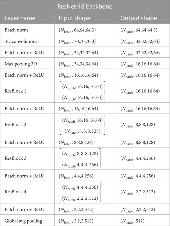
TABLE 1. Configuration of the backbone BNNs used for all experiments presented in this paper.

FIGURE 1

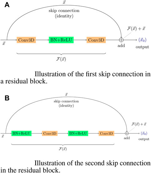
FIGURE 1. Each ResBlock includes both skip connection configurations. (A) ResBlock starts with this configuration applied to the input tensor. (B) Output of the previous configuration is fed into this connection.

The loss function to be optimized during training is given by ELBO 2, where the second term is associated with the negative log-likelihood (NLL)

$-\text{NLL}\sim \frac{1}{2}\log |s\cdot \mathrm{\Sigma }|+\frac{1}{2}{\left(\mathbf{y}-\mu \right)}^{\top }{\left(s\cdot \mathrm{\Sigma }\right)}^{-1}\left(\mathbf{y}-\mu \right)(12)$

averaged over the mini-batch. The scalar variable s is equal to one during the training process, and it becomes a trainable variable during post-training to recalibrate the probability density function (Hortúa et al., 2020b; Laves et al., 2020). The optimizer used to minimize the objective function is the Adam with first and second moments exponential decay rates of 0.9 and 0.999, respectively Kingma and Ba (2014). The learning rate starts from 10⁻³, and it will be reduced by a factor of 0.8 in case any improvement has not been observed after 10 epochs. Furthermore, we have applied a warm-up period for which the model turns on progressively the KL term in Eq. 2. This is achieved by introducing a β variable in the ELBO, i.e., $\beta \cdot \text{KL}\left[q(w|\theta )‖p(w)\right]$; so, this parameter starts being equal to 0 and grows linearly to 1 during 10 epochs (Sønderby et al., 2016). BNNs were trained with 32 batches and early stopping callback to avoid overfitting. The infrastructure put in place by the Google Cloud Platform (GCP) uses NVIDIA-Tesla-T4 of 16 GB GDDR6 in an N1 machine series shared-core.

4.1 Metrics

We compare all BNN results in terms of performance, i.e., the precision of their predictions for the cosmological parameters quantified through mean square error (MSE), ELBO, and plotting the true vs. predicted values with its coefficient of determination. Moreover, it is important to quantify the quality of the uncertainty estimates. One of the ways to diagnose the quality of the uncertainty estimates is through reliability diagrams. Following the work of Laves et al. (2020) and Guo et al. (2017), we can define a perfect calibration of regression uncertainty as follows:

${\mathbb{E}}_{{\widehat{\sigma }}^2}\left[\text{abs}\left[\left(\Vert \mathit{y}-\mathit{\mu }{\Vert }^2\left|{\widehat{\sigma }}^2={\alpha }^2\right.\right)-{\alpha }^2\right]\right]\forall \left\{{\alpha }^2\in \mathbb{R}\left|{\alpha }^2\ge 0\right.\right\},(13)$

abs [.] being the absolute value function. Hence, the predicted uncertainty ${\widehat{\sigma }}^2$ is partitioned into K bins with equal width, and the variance per bin is defined as follows:

$\mathrm{v}\mathrm{a}\mathrm{r}\left(B_k\right)≔\frac{1}{\left|B_k\right|}\sum _{i\in B_m}\frac{1}{N}\sum _{n=1}^N{\left({\mathit{\mu }}_{i,n}-{\mathit{y}}_i\right)}^2,(14)$

with N stochastic forward passes. On the other hand, the uncertainty per bin is defined as follows:

$\mathrm{u}\mathrm{n}\mathrm{c}\mathrm{e}\mathrm{r}\mathrm{t}\left(B_k\right)≔\frac{1}{|B_k|}\sum _{i\in B_k}{\widehat{\sigma }}_i^2.(15)$

With these two quantities, we can generate reliability diagrams to evaluate the quality of the estimated uncertainty via plotting var (B_k) vs. uncert (B_k). In addition, we can compute the expected uncertainty calibration error (UCE) in order to quantify the miscalibration

$\mathrm{U}\mathrm{C}\mathrm{E}≔\sum _{k=1}^K\frac{|B_k|}{m}\left|\mathrm{v}\mathrm{a}\mathrm{r}\left(B_k\right)-\mathrm{u}\mathrm{n}\mathrm{c}\mathrm{e}\mathrm{r}\mathrm{t}\left(B_k\right)\right|,(16)$

with the number of inputs m and set of indices B_k of inputs, for which the uncertainty falls into the bin k. A more general approach proposed by Hortúa et al. (2020b) consists in computing the expected coverage probabilities defined as the x% of samples for which the true value of the parameters falls in the x%-confidence region defined by the joint posterior. Clearly, this option is more precise since it captures higher-order statistics through the full posterior distribution. However, for simplicity, we will follow the UCE approach.

5 Analysis and results of parameter inference with BNNs

In this section, we discuss the results obtained by comparing three different versions of BNNs, the one with MNFs, the standard BNN, and the third one using Flipout as an estimator. The results reported in this section were computed on the test dataset. Table 2 shows the metrics obtained for each BNN approach. As mentioned, MSE, ELBO, and r² provide good estimates for determining the precision of the model, while UCE measures the miscalibration. It should be noted that VBNNs outperform all experiments taking into account not only the average error but also the precision for each cosmological parameter along with a good calibration in its uncertainty predictions. Followed by VBBNs, we have the FlipoutBNNs; although this approach yields good cosmological parameter estimation, it underestimates their uncertainties. Therefore, VBNNs avoid the application of an extra post-training step in the machine learning pipeline related to calibration. It should be noted that in all experiments, h becomes hardly predicted for all models. Figure 2 displays the true against the predicted values for Ω_m, ω_m (instead of h), σ₈, and the degeneracy direction defined as ${\sigma }_8{\mathrm{\Omega }}_m^{0.25}$. Error bars report the epistemic plus aleatoric uncertainties predicted by BNNs, which illustrate the advantages of these probabilistic models where the certainty prediction of the model is captured instead of traditional DNNs where only point estimates are present. This uncertainty was taken from the diagonal part of the covariance matrix.

TABLE 2

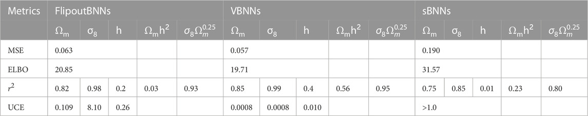
TABLE 2. Metrics for the test set for all BNN architectures. High UCE values indicate miscalibration. MSE and ELBO are computed only over the cosmological parameters.

FIGURE 2

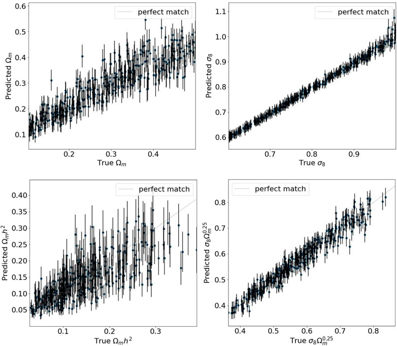
FIGURE 2. Plots of true vs. predicted values provided by the best experiment VBNNs, for Ω_m, σ₈, and some derivative parameters. Points are the mean of the predicted distributions, and error bars stand for the heteroscedastic uncertainty associated with epistemic plus aleatoric uncertainties at 1σ.

5.1 Calibration metrics

In Figure 3, we analyze the quality of our uncertainty measurement using calibration diagrams. We show the predicted uncertainty vs. observed uncertainty from our model on the test dataset.

FIGURE 3

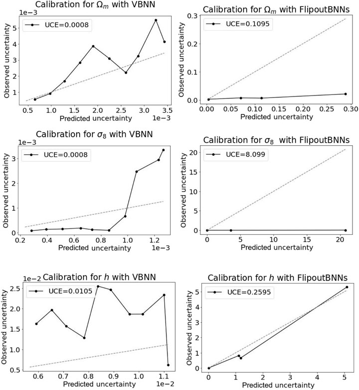
FIGURE 3. Calibration diagrams for the best experiments, VBNNs and FlipoutBNNs. The lower the UCE value, the higher the calibration of the model. Dashes lines stand for the perfect calibration, so the discrepancy to this identity curve reveals miscalibration.

Better performing uncertainty estimates should correlate more accurately with the dashed lines. We can see that estimating uncertainty from VBNNs reflects the real uncertainty better. Furthermore, the UCE value for VBNNs is much lower than the one obtained by FlipoutBNN, which also implies how reliable this model according to their predictions is. It should be noted that even if we partitioned the variance into K = 10 bins with equal width, FlipoutBNNs and sBNNs yield underestimate uncertainties (many examples concentrate in lower bin values); for this reason, we see that while VBNNs supply all 10 samples in the calibration plots, for the others, we have just 3–4 of them. Next, we employed the σ-scaling methodology for calibrating the FlipoutBNN predictions (Laves et al., 2020). At doing so, we optimize only the loss function described in Eq. 12 where all parameters related to the BNNs were frozen, i.e., the only trainable parameter was s. After training, we got s ∼ 0.723, reducing UCE only up to 10%, and the number of samples in the calibration diagrams enlarged to 4–5. This minor performance enhancement means that σ-scaling is not suitable to calibrate all BNNs, and alternative re-calibration techniques must be taken into account in order to build reliable intervals. At this point, we have noticed the advantages of working with methods that lead to networks already well-calibrated after the training step (Hortúa et al., 2020a).

5.2 Joint analysis for cosmological parameters

In order to show the parameter intervals and contours from the N-body simulations, we randomly choose an example from the test set with true values shown in Table 3. The two-dimensional posterior distribution of the cosmological parameters is shown in Figure 4, and the parameter 95% intervals are reported in Table 3. It should be noted that VBNNs provide considerably tighter and well constraints on all parameters with respect to the sBNNs reported by Hortua (2021). Most importantly, this technique also offers the correlation among parameters and the measurement of how reliable the model is in their predictions.

TABLE 3

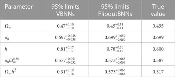
TABLE 3. Parameter 95% intervals taken from the parameter constraint contours (Figure 4) from one example of the QUIJOTE test dataset using VBNNs and FlipoutBNNs.

FIGURE 4

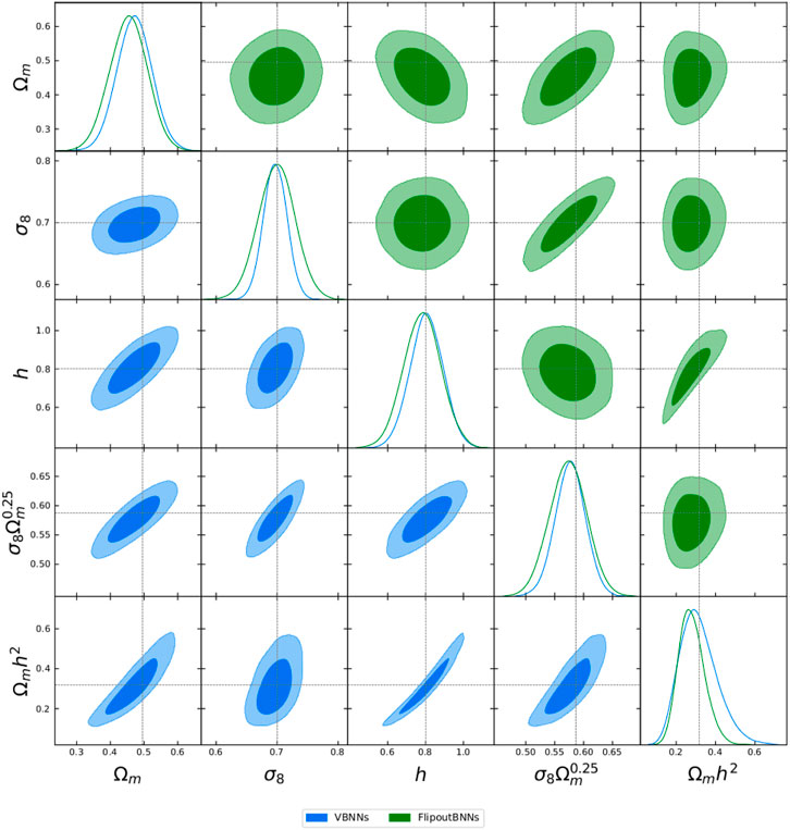
FIGURE 4. 68% and 95% parameter constraint contours from one example of the QUIJOTE test dataset using VBNNs and FlipoutBNNs. The diagonal plots are the marginalized parameter constraints, and the dashed lines stand for the true values. We derive these posterior distributions using GetDist (Lewis, 2019).

6 Conclusion

N-body simulations offer one of the most powerful ways to understand the initial conditions of the Universe and improve our knowledge of fundamental physics. In this paper, we used the QUIJOTE dataset to show how convolutional DNNs capture non-Gaussian patterns without requiring a specifying summary statistic (such as PS). Additionally, we have shown how we can build probabilistic DNNs to obtain uncertainties that generate reliable predictions. One of the main goals of this paper was also to report the degree of improvement achieved by BNNs when we integrate with techniques such as MNFs to enhance the variational posterior complexity. We found that VBNNs not only provide considerably tighter and well constraints on all cosmological parameters as we observed in Figure 4 but also yield well-calibrated estimate uncertainties as shown in Figure 3. Although the approach used in this paper was based only on the Bayesian multilayer perceptron (B-MLP), this method is also expanded to 2D convolutions, B-CNN (Louizos and Welling, 2017). Hence, these results can be applied to other probes such as galaxy photometric redshift (CfA Redshift Survey) and large spectroscopic surveys (SDSS, DES, or LSST). Building those B-MLP and B-CNNs for additional extensions to Λ-CDM will be beneficial to reveal the presence of new physics in cosmological datasets. Nevertheless, some limitations in this research include simple prior assumptions (mean-field approximations), lower resolution in the simulations, and the absence of additional calibration techniques. These restrictions will be analyzed in detail in a future paper.

Data availability statement

Publicly available datasets were analyzed in this study. These data can be found at: https://quijote-simulations.readthedocs.io/en/latest/.

Author contributions

HH: conceptualization, methodology, and software. LG: data collection, validation, writing—original draft preparation, and cosmological analysis. LC: conceptualization and cosmological analysis. All authors contributed to the article and approved the submitted version.

Funding

This paper is based on work supported by the Google Cloud Research Credits program with the award GCP19980904. LC was supported by patrimonio autónomo fondo Nacional de financiamiento para la ciencia y la tecnología y la innovacion Francisco José de Caldas (Minciencias Colombia) grant no. 110685269447 RC-80740-465-2020 projects 69723.

Acknowledgments

HH acknowledges support from créditos educación de doctorados nacionales y en el exterior- Colciencias and the grant provided by the Google Cloud Research Credits program.

Conflict of interest

The authors declare that the research was conducted in the absence of any commercial or financial relationships that could be construed as a potential conflict of interest.

Publisher’s note

All claims expressed in this article are solely those of the authors and do not necessarily represent those of their affiliated organizations, or those of the publisher, the editors, and the reviewers. Any product that may be evaluated in this article, or claim that may be made by its manufacturer, is not guaranteed or endorsed by the publisher.

Footnotes

¹The targets $y\in {\mathbb{R}}^N$.

²The parameter θ will be omitted in this section for clarity of notation.

References

Abadi, M., Agarwal, A., Barham, P., Brevdo, E., Chen, Z., Citro, C., et al. (2015). TensorFlow: Large-scale machine learning on heterogeneous systems Software available from tensorflow.org.

Google Scholar

Abdalla, E., Abell’an, G. F., Aboubrahim, A., Agnello, A., Akarsu, O., Akrami, Y., et al. (2022). Cosmology intertwined: A review of the particle physics, astrophysics, and cosmology associated with the cosmological tensions and anomalies. J. High Energy Astrophysics34, 49–211. doi:10.1016/j.jheap.2022.04.002

CrossRef Full Text | Google Scholar

Abdar, M., Pourpanah, F., Hussain, S., Rezazadegan, D., Liu, L., Ghavamzadeh, M., et al. (2021). A review of uncertainty quantification in deep learning: Techniques, applications and challenges. Inf. Fusion76, 243–297. doi:10.1016/j.inffus.2021.05.008

CrossRef Full Text | Google Scholar

Chang, D. T. (2021). Bayesian neural networks: Essentials. doi:10.48550/ARXIV.2106.13594

CrossRef Full Text | Google Scholar

Charnock, T., Perreault-Levasseur, L., and Lanusse, F. (2020). Bayesian neural networks. doi:10.48550/ARXIV.2006.01490

CrossRef Full Text | Google Scholar

Dinh, L., Sohl-Dickstein, J., and Bengio, S. (2017). “Density estimation using real NVP,” in International conference on learning representations.

Google Scholar

Dodelson, S. (2003). Modern cosmology. Academic Press, Elsevier Science.

Google Scholar

Dvorkin, C., Mishra-Sharma, S., Nord, B., Villar, V. A., Avestruz, C., Bechtol, K., et al. (2022). Machine learning and cosmology. doi:10.48550/ARXIV.2203.08056

CrossRef Full Text | Google Scholar

Gal, Y. (2016). Uncertainty in deep learning. Ph.D. thesis, University of Cambridge.

Google Scholar

Gillet, N., Mesinger, A., Greig, B., Liu, A., and Ucci, G. (2019). Deep learning from 21-cm tomography of the cosmic dawn and reionization. Mon. Notices R. Astronomical Soc.484, 282–293. doi:10.1093/mnras/stz010

CrossRef Full Text | Google Scholar

A. Graves (Editor) (2011). Practical variational inference for neural networks (Curran Associates, Inc.), 24.

Google Scholar

Gunapati, G., Jain, A., Srijith, P. K., and Desai, S. (2022). Variational inference as an alternative to mcmc for parameter estimation and model selection. Publ. Astronomical Soc. Aust.39, e001. doi:10.1017/pasa.2021.64

CrossRef Full Text | Google Scholar

Guo, C., Pleiss, G., Sun, Y., and Weinberger, K. Q. (2017). “On calibration of modern neural networks,” in Proceedings of the 34th international conference on machine learning - volume 70 (JMLR.org) (ICML), 17, 1321–1330.

Google Scholar

Hamann, J., Hannestad, S., Lesgourgues, J., Rampf, C., and Wong, Y. Y. (2010). Cosmological parameters from large scale structure - geometric versus shape information. J. Cosmol. Astropart. Phys.2010, 022. doi:10.1088/1475-7516/2010/07/022

CrossRef Full Text | Google Scholar

Hortua, H. J. (2021). Constraining cosmological parameters from n-body simulations with Bayesian neural networks. doi:10.48550/ARXIV.2112.11865

CrossRef Full Text | Google Scholar

Hortúa, H. J., Malagò, L., and Volpi, R. (2020a). Constraining the reionization history using Bayesian normalizing flows. Mach. Learn. Sci. Technol.1, 035014. doi:10.1088/2632-2153/aba6f1

CrossRef Full Text | Google Scholar

Hortúa, H. J., Volpi, R., Marinelli, D., and Malagò, L. (2020b). Parameter estimation for the cosmic microwave background with Bayesian neural networks. Phys. Rev. D.102, 103509. doi:10.1103/physrevd.102.103509

CrossRef Full Text | Google Scholar

Kendall, A., and Gal, Y. (2017). What uncertainties do we need in Bayesian deep learning for computer vision?

Google Scholar

Kingma, D. P., and Ba, J. (2014). Adam: A method for stochastic optimization. doi:10.48550/ARXIV.1412.6980

CrossRef Full Text | Google Scholar

Kirichenko, P., Izmailov, P., and Wilson, A. G. (2020). “Why normalizing flows fail to detect out-of-distribution data,” in Proceedings of the 34th international conference on neural information processing systems (Red Hook, NY, USA: Curran Associates Inc.). NIPS’20.

Google Scholar

Kiureghian, A. D., and Ditlevsen, O. (2009). Aleatory or epistemic? Does it matter?Struct. Saf.31, 105–112. doi:10.1016/j.strusafe.2008.06.020

CrossRef Full Text | Google Scholar

Kwon, Y., Won, J.-H., Joon Kim, B., and Paik, M. (2018). in International conference on medical imaging with deep learning, 13.

Google Scholar

Laves, M.-H., Ihler, S., Fast, J. F., Kahrs, L. A., and Ortmaier, T. (2020). “Well-calibrated regression uncertainty in medical imaging with deep learning,” in Medical imaging with deep learning.

Google Scholar

Lazanu, A. (2021). Extracting cosmological parameters from n-body simulations using machine learning techniques. J. Cosmol. Astropart. Phys.2021, 039. doi:10.1088/1475-7516/2021/09/039

CrossRef Full Text | Google Scholar

Lewis, A. (2019). GetDist: A Python package for analysing Monte Carlo samples.

Google Scholar

List, F., Rodd, N. L., Lewis, G. F., and Bhat, I. (2020). Galactic center excess in a new light: Disentangling the gamma-ray sky with Bayesian graph convolutional neural networks. Phys. Rev. Lett.125, 241102. doi:10.1103/physrevlett.125.241102

PubMed Abstract | CrossRef Full Text | Google Scholar

Louizos, C., and Welling, M. (2017). “Multiplicative normalizing flows for variational Bayesian neural networks,” in Proceedings of the 34th international conference on machine learning - volume 70 (JMLR.org) (ICML’17), 2218–2227.

Google Scholar

Mancarella, M., Kennedy, J., Bose, B., and Lombriser, L. (2022). Seeking new physics in cosmology with Bayesian neural networks: Dark energy and modified gravity. Phys. Rev. D.105, 023531. doi:10.1103/PhysRevD.105.023531

CrossRef Full Text | Google Scholar

Mesinger, A., Furlanetto, S., and Cen, R. (2011). 21cmfast: A fast, seminumerical simulation of the high-redshift 21-cm signal. Mon. Notices R. Astronomical Soc.411, 955–972. doi:10.1111/j.1365-2966.2010.17731.x

CrossRef Full Text | Google Scholar

Nalisnick, E., Matsukawa, A., Teh, Y. W., Gorur, D., and Lakshminarayanan, B. (2019). “Do deep generative models know what they don’t know?,” in International conference on learning representations.

Google Scholar

Planck, C., Aghanim, N., Akrami, Y., Ashdown, M., Aumont, J., Baccigalupi, C., et al. (2020). Planck 2018 results. Astronomy Astrophysics641, A6. doi:10.1051/0004-6361/201833910

CrossRef Full Text | Google Scholar

Ranganath, R., Tran, D., and Blei, D. M. (2016). “Hierarchical variational models,” in Proceedings of the 33rd international conference on international conference on machine learning - volume 48 (JMLR.org) (ICML’16), 2568–2577.

Google Scholar

Ravanbakhsh, S., Oliva, J., Fromenteau, S., Price, L. C., Ho, S., Schneider, J., et al. (2017). Estimating cosmological parameters from the dark matter distribution. doi:10.48550/ARXIV.1711.02033

CrossRef Full Text | Google Scholar

Scoccimarro, R. (1998). Transients from initial conditions: A perturbative analysis. Mon. Notices R. Astronomical Soc.299, 1097–1118. doi:10.1046/j.1365-8711.1998.01845.x

CrossRef Full Text | Google Scholar

Solovyev, R., Kalinin, A. A., and Gabruseva, T. (2022). 3d convolutional neural networks for stalled brain capillary detection. Comput. Biol. Med.141, 105089. doi:10.1016/j.compbiomed.2021.105089

PubMed Abstract | CrossRef Full Text | Google Scholar

Sønderby, C. K., Raiko, T., Maaløe, L., Sønderby, S. K., and Winther, O. (2016). “Ladder variational autoencoders,” in Proceedings of the 30th international conference on neural information processing systems (Red Hook, NY, USA: Curran Associates Inc). NIPS’16, 3745–3753.

Google Scholar

Springel, V. (2005). The cosmological simulation code gadget-2. Mon. Notices R. Astronomical Soc.364, 1105–1134. doi:10.1111/j.1365-2966.2005.09655.x

CrossRef Full Text | Google Scholar

Stefano, B., and Kravtsov, A. (2011). Cosmological simulations of galaxy clusters. Adv. Sci. Lett.4, 204–227. doi:10.1166/asl.2011.1209

CrossRef Full Text | Google Scholar

Tinker, J. L., Sheldon, E. S., Wechsler, R. H., Becker, M. R., Rozo, E., Zu, Y., et al. (2011). Cosmological constraints from galaxy clustering and the mass-to-number ratio of galaxy clusters. Astrophysical J.745, 16. doi:10.1088/0004-637x/745/1/16

CrossRef Full Text | Google Scholar

Touati, A., Satija, H., Romoff, J., Pineau, J., and Vincent, P. (2018). Randomized value functions via multiplicative normalizing flows. doi:10.48550/ARXIV.1806.02315

CrossRef Full Text | Google Scholar

Villaescusa-Navarro, F., Hahn, C., Massara, E., Banerjee, A., Delgado, A. M., Ramanah, D. K., et al. (2020). The quijote simulations. Astrophysical J. Suppl. Ser.250, 2. doi:10.3847/1538-4365/ab9d82

CrossRef Full Text | Google Scholar

Wagner-Carena, S., Park, J. W., Birrer, S., Marshall, P. J., Roodman, A., and Wechsler, R. H. (2021). Hierarchical inference with Bayesian neural networks: An application to strong gravitational lensing. Astrophysical J.909, 187. doi:10.3847/1538-4357/abdf59

CrossRef Full Text | Google Scholar

Wang, B. Y., Pisani, A., Villaescusa-Navarro, F., and Wandelt, B. D. (2022). Machine learning cosmology from void properties. doi:10.48550/ARXIV.2212.06860

CrossRef Full Text | Google Scholar

Wen, Y., Vicol, P., Ba, J., Tran, D., and Grosse, R. (2018). Flipout: Efficient pseudo-independent weight perturbations on mini-batches. doi:10.48550/ARXIV.1803.04386

CrossRef Full Text | Google Scholar

Yusofi, E., and Ramzanpour, M. A. (2022). Cosmological constant problem and h₀ tension in void-dominated cosmology. doi:10.48550/ARXIV.2204.12180

CrossRef Full Text | Google Scholar