Models of thermal conduction and non-local transport of relevance to space physics with insights from laser–plasma theory

1 Introduction

The energy balance of the solar chromosphere, transition region, and corona is determined by the energy input, transport, and radiation. The energy input can be diffused and steady from, for example, wave heating, or can be rapid and localised from flares. Flares themselves cover a range of energies and timescales from nanoflares to large X-class events. Irrespective of the time and length scale of the energy input, it will always be transported, primarily along the magnetic field lines. This energy transport is the origin of white light and X-ray emission from the chromosphere, and the balance between these heating mechanisms and optically thin radiative losses determines the location and structure of the transition region. With 3D modelling of the solar corona playing an increasingly important role in the study of coronal heating and flares, it is important that the best models for this energy transport are used. There are, however, always compromises to be made, and a full Vlasov–Fokker–Planck (VFP) treatment of this transport is computationally intractable on length scales and timescales probed by 3D MHD simulations. This paper reviews the options available for reduced thermal transport models, from localised models to non-local transport. Much of this recent work has been undertaken by the laser–plasma community in order to improve the accuracy of predictive models for laser-driven fusion. Here, we not only review models in common use by the solar community but also give outlines of the methods used in laser–plasmas that may be of benefit to next-generation coronal simulations.

The coronal temperature is typically in the range 1–10 MK. The temperature length scales can be of or over 10 Mm for a steady uniform heating model and can be down to about 100 km in the transition region. Shorter scale lengths may still be generated in nanoflare heating models. The important parameter for determining the optimal heat flux model is the Knudsen number $K_n={\lambda }_{ei}^{\text{T}}/L_T$. Here, ${\lambda }_{ei}^{\text{T}}$ is the thermal electron mean-free path, i.e., the characteristic scale over which electron collisions are important for electrons moving at the thermal speed, and L_T = T/|∇T| is the temperature scale length. Thermal transport is usually dominated by electrons, so here, we ignore the ion transport effects. For a 1 MK coronal plasma, with a number density of 10¹⁵ m⁻³, the electron mean-free path based on the local thermal speed is approximately 50 km, while for 10 MK, it is around 5 Mm. We will see below that local transport models begin to fail when K_n > 0.01, not when K_n > 1, as is often mistakenly assumed. As a result, for a 1 MK plasma, the local approximation fails on length scales less than about 5 Mm, while for a 10 MK plasma, it fails for scales less than 500 Mm. As a result, it is possible that for a quiet corona at 1 MK, the local Spitzer–Harm (Spitzer and Härm, 1953) approach is valid, except in a small section of the transition region. For any MHD scale modelling of flares, however, it is extremely unlikely that the Spitzer–Harm model is correct. Indeed, the observations of wave damping indicate that thermal transport is reduced relative to the Spitzer–Harm conductivity in the solar corona (Wang et al., 2018).

It is important when discussing energy transport in the solar corona, especially in the active regions, to be clear of the distinction between thermal and non-thermal transport. Thermal transport arises from perturbations of the distribution due to a temperature gradient. This can only be a sensible physical model if the distribution function is close enough to being Maxwellian that temperature is a meaningful statistical tool for describing that distribution. It is always possible to define temperature from the second moment of a distribution, but this is not helpful unless that distribution is close to the local thermal equilibrium. Some models, such as the Schurtz–Nicolai–Busquet (SNB) model described below, are based on an expansion of the distribution function to first order, and as a result, when K_n > 1, this is unlikely to be satisfied. New models, which are expected to be valid for lower K_n, have recently been developed (Del Sorbo et al., 2015), but their accuracy and computational efficiency are yet to be assessed. What cannot be handled by any thermal transport model are beams or significant deviations from a Maxwellian distribution function. Here, the temperature of the whole distribution is not a meaningful measure, and hence, the transport of energy in such cases is non-thermal and not covered in this article. We are primarily interested in what is possible within the MHD approximation, where temperature and pressure are sensible fluid moments.

This paper first covers local transport and the Spitzer–Harm, also often called Braginskii, thermal conduction. This section highlights the importance of the Knudsen number and velocity dependence of the mean-free path. The Knudsen number is used to define the limits of local transport and the breakdown of classical Spitzer–Harm thermal conduction on the MHD scale. Models to handle conduction, when the local approximation is not valid, include flux limiters, models using non-local kernels, and the current state-of-the-art from laser-plasma theory. All equations presented in this article use S.I. units.

2 Local thermal transport

A full derivation of the local approximation thermal conductivity is not needed in order to understand the limitations of this theory. Here, for simplicity, we sketch a derivation for a simplified collision operator, as this highlights all the key physics. All electron transport coefficients can be determined by solving the electron distribution function f from the VFP equation.

$\frac{\partial f}{\partial t}+\mathbf{v}.\nabla f-\frac{e}{m_e}\left(\mathbf{E}+\mathbf{v}\times \mathbf{B}\right).{\nabla }_{v}f={\left(\frac{\partial f}{\partial t}\right)}_c,(1)$

where the right-hand side represents the change in f due to collisions, E is the electric field, B is the magnetic field, and v is the phase-space velocity coordinate. In this paper, we restrict attention to thermal transport along the magnetic field and, thus, drop the v × B term and restrict the velocity to the component along the magnetic field v. The two components of the heat flux perpendicular to the magnetic field have conductivities smaller than the parallel conductivity by factors of $1/{\omega }_{ce}{\tau }_e^T$ and $1/{({\omega }_{ce}{\tau }_c^T)}^2$. Here, ω_ce = eB/m_e is the electron cyclotron frequency, and ${\tau }_c^T$ is the electron collision time defined using the electron thermal speed. In most space plasmas, ${\omega }_{ce}{\tau }_c^T>10^6$.

Ideally, Eq. 1 would be solved using the full Fokker–Planck collision operator, but for illustrative purposes, here, we use a simple relaxation operator that returns the distribution function to local Maxwellian f_M on a collisional timescale τ_c, given as follows:

${\left(\frac{\partial f}{\partial t}\right)}_c=-\frac{\left(f-f_M\right)}{{\tau }_c},(2)$

with f_M, the local Maxwellian distribution function. In general, the collision time τ_c is a function of electron speed and from basic plasma theory τ_c ∝ v³. Once we have a solution for f, we can immediately determine the heat flux from the following:

${\mathbf{Q}}_{\mathbf{e}}=\int \left(\frac{1}{2}{m}_e{v}^2\right)\mathbf{v}f{d}^3\mathbf{v}.(3)$

It should be noted that while Eq. 3 is the general vector heat flux here, we restrict attention to the magnitude of this heat flux Q_e along the magnetic field. The advantage of the simplified collision operator is that under the assumption of a fixed, imposed temperature gradient and an equilibrium state, we immediately get the solution for f as follows:

$f=f_M-{\tau }_{c}v\frac{\partial f}{\partial x}+\frac{{\tau }_{c}e}{m_e}E\frac{\partial f}{\partial v}.(4)$

It is at this stage that the local approximation is made. We expand f as a perturbation of the distribution function so that f = f_M + f₁ and linearise Eq. 4. Estimating ∂_xf ≃ f/L, with L being the scale length of interest, we see the following:

${\tau }_{c}v\frac{\partial f}{\partial x}\sim \frac{{\tau }_{c}v}{L}f(5)$

so that if τ_cv/L is small, i.e., first order, and E is also first order, then

$f_1=-{\tau }_{c}v\frac{\partial f_M}{\partial x}+\frac{{\tau }_{c}e}{m_e}E\frac{\partial f_M}{\partial v}.(6)$

The electric field is determined under the condition that the heat flux cannot drive a current, ensuring that the plasma remains quasi-neutral. The distribution function, as a result of the heat flux, is then fully determined. If we assume that τ_c is not a function of speed and replace τ_c with ${\tau }_c^T$, then this procedure gives a heat flux of Q_e = −κ∇T_e with $\kappa =5n_e{k}_{\text{B}}^2{T}_{\text{e}}{\tau }_c^T/(2m_e)$. Here, the electron collisional timescale is ${\tau }_c=12\sqrt{m_e}{\pi }^{3/2}{\epsilon }_0^2{\left(k_{B}T\right)}^{3/2}/(\sqrt{2}Z{n}_e{\lambda }_{ei}{e}^4)$. This is a reasonable estimate of the heat flux, but the full answer in this local approximation must be obtained through the velocity-dependent VFP collision term. For the solar coronal plasma, the final heat flux is often approximated as follows:

$Q_e=-10^{-11}{T}_{\text{e}}^{5/2}{\nabla }_{\Vert }{T}_{\text{e}}.(7)$

It is based on using the Braginskii (Spitzer–Harm) conductivity and the choice of the Coulomb logarithm ≃ 20. Here, the gradient operator ∇_‖ is along a guiding magnetic field, so that ∇_‖T_e is scalar. These assumptions will be used throughout this article.

If the plasma is collision-dominated, then Eq. 7 is a good approximation for thermal conduction in the solar corona. Crucially, however, this requires that the dimensionless parameter τ_cv/L is small. For conduction, we can take L = L_T, but we need to specify τ_c. By definition, the mean-free path is λ_ei = τ_cv. In general, λ = τv, so that λ_ei = λ_ei(v) and ${\lambda }_{ei}^{\text{T}}={\lambda }_{ei}(v_{\text{T}})$, where we take the thermal speed as $v_{\text{T}}^2=k_{\text{B}}{T}_e/m_e$. The electron mean-free path (not averaged over the distribution) is proportional to v⁴, so that the following is observed:

${\lambda }_{ei}={\left(\frac{v}{v_{\text{T}}}\right)}^4{\lambda }_{ei}^{\text{T}}.(8)$

The heat flux is determined by high-order moments of the perturbed electron distribution function, and for near-Maxwellian plasmas, it is dominated by electrons in the distribution with speeds in the range of 2.5–3.5 v_T. These are the electron speeds for which the integrand in Eq. 3 is the largest. The mean-free path of these electrons is 40–150 times the thermal mean-free path. For this reason, the local approximation used to derive Q_e; i.e., the term in Eq. 5 is a first-order quantity, breaks down for electrons with speeds of 2.5–3.5 v_T, when K_n > 0.01 and not when K_n > 1.

3 Flux limiters

For a coronal plasma, a good approximation for the electron thermal mean-free path is as follows:

${\lambda }_{ei}^{\text{T}}=5.5\times 10^7\left(\frac{T^2}{n_e}\right),(9)$

which can be used to rewrite the heat flux as follows:

$Q_e=-3.2\left(n_e{k}_{\text{B}}T\right)v_{\text{T}}\frac{{\lambda }_{ei}^{\text{T}}}{L_{\text{T}}}.(10)$

The free-streaming limit is defined as Q_fs = n_ek_BTv_T, and it corresponds to the heat flux if the local thermal energy density (n_ek_BT) is advected at the thermal speed. This is clearly a sensible estimate for the upper limit of the heat flux for a near-Maxwellian plasma. In addition, as noted previously, the thermal flux is not carried by the whole electron distribution, but it is dominated by the fraction of electrons with speeds of 2.5–3.5 v_T. Flux limiters aim to account for these natural limits by restricting the heat flux to being less than some multiple of Q_fs. Most commonly, in explicit treatments of thermal conduction, this would be implemented by defining a limited heat flux through the following:

$\frac{1}{Q_e}=\frac{1}{Q_{SH}}+\frac{1}{\alpha Q_{fs}}.(11)$

The factor α is called the flux limiter and in laser–plasma modelling is typically between 0.05 and 0.2, for example, in the study by Jones et al. (2017), and Q_SH is the heat flux predicted by the Spitzer–Harm approach. It should be noted, however, that these values are arrived at by varying α to get the best agreement between simulations and observations. This is a purely empirical fix and is problem-dependent. In the solar wind, for example, it is typical to use α ≃ 1 (van der Holst et al., 2014), while in tokamak scrape-off layers, limiters up to α ≃ 3 are used (Fundamenski, 2005).

3D flare models using a flux limiter (Cheung et al., 2019) with α = 1/6 have shown that this may reproduce a power-law X-ray spectrum from purely Maxwellian electrons. 1D models require a power-law, high-energy component of the electron distribution to match the observed X-ray spectrum. However, different regions of the flaring 3D atmosphere reach different temperatures at different times. The sum of the contributions from this multi-thermal, dynamic atmosphere may give rise to an integrated X-ray spectrum, which resembles a power law. Assessing this result is beyond the scope of this article, but the study by Cheung et al. (2019) is an example of active region modelling where an improved thermal transport model is needed.

4 Non-local kernel models

The α parameter in the flux-limited model needs to be determined based on a best fit for observations, and so, it has limited predictive capacity. The second issue is that as the Knudsen number increases, the heat flux becomes non-local, i.e., it no longer depends on the local temperature gradient. Any non-local model for conduction must capture two important effects. First, it must naturally give rise to a limited flux without the need for an ad hoc, semi-empirical limiter. Second, it must correctly model preheat. This is where the most energetic electrons transport heat faster than bulk thermal conduction. This occurs as the most energetic electrons have the longest mean-free paths, and this effect is not captured by flux limiters. The non-local energy transport models used in solar 1D ((Karpen and Devore, 1987; West et al., 2004)) and 3D (Silva et al., 2018) models have relied on the kernel model derived for laser–plasmas (Luciani et al., 1983), commonly referred to as the LMV model. In this model, the heat flux is calculated by convolving the local conduction with a non-local kernel. This gives the following heat flux:

$Q_e\left(x\right)=\int w\left(x,x^{\prime }\right)Q_{sh}\left(x^{\prime }\right)d{x}^{\prime },(12)$

where w (x, x′) is a kernel used to introduce non-local effects. The kernel used in the LMV model is as follows:

$w\left(x,x^{\prime }\right)=\frac{1}{2a{\lambda }_{ei}^{\text{T}}\left(x^{\prime }\right)}\exp \left(-\frac{{\int }_x^{x^{\prime }}{n}_e\left(y\right)dy}{2a{n}_e\left(x^{\prime }\right){\lambda }_{ei}^{\text{T}}\left(x^{\prime }\right)}\right).(13)$

The free parameter a is set in LMV to 32 to get a best fit to VFP simulations. Other kernels are possibly based on simplified collision operators. Thus, kernel-based models are able to capture the non-local effect, but there remain free parameters, such as a in the LMV model, and there is no unique choice of kernel universally proven to be optimal in all conditions. 3D flare simulations (Silva et al., 2018) have included LMV style non-local electron transport in MHD flare models and shown that this significantly changes the predictions for the temperature of the transition region and upper chromosphere.

5 The SNB model

The LMV model was originally derived in the context of laser-produced plasmas, where large mean-free paths are common. LMV has been superseded in laser–plasma modelling by the SNB model (Schurtz et al., 2000) as the most efficient way to treat non-local transport while maintaining fluxes close to those from VFP on the MHD scale. The SNB model has been verified against full VFP simulations (Marocchino et al., 2013; Brodrick et al., 2017; Sherlock et al., 2017). The SNB model is now routinely used in laser–plasma radiation hydrodynamic codes, e.g., in the study by Farmer et al. (2018). It has also been shown to be more accurate than models used in simulations of magnetically confined fusion plasmas (Brodrick et al., 2017), where non-local transport plays an important role in heat exhausts (Omotani and Dudson, 2013; Wigram et al., 2020). It lacks the full detail of a VFP solution (impractical in 3D simulations) but does reproduce the non-local preheat and flux-limiting properties well for temperature profiles one would expect in the corona. The advantage of SNB over LMV is that it is easier to implement in 3D models. LMV requires tracing 3D magnetic field lines and applying the LMV non-local model along enough field lines to reconstruct the temperature in 3D, whereas SNB involves solving PDEs. Also, there is no need to choose a kernel function or set free parameters; SNB is a predictive and self-contained theory.

The SNB model can be derived from VFP, and outlines of this derivation can be found in studies by Schurtz et al. (2000) and Brodrick et al. (2017). The essential feature of this method is that the VFP equation is approximated in energy bins. These energy bins, usually uniformly distributed, span the distribution function. The solutions in these bins are combined to calculate a correction to the local heat flux. The full equation set from this energy discretisation for the non-local heat flux Q_nl is as follows:

$Q_{nl}=Q_{SH}-\sum _g\frac{{\lambda }_g}{3}\nabla H_g(14)$

with ${\lambda }_g^2={\lambda }_{ei}{\lambda }_{ee}$ being defined for each energy group E_g. The functions H_g are found for each energy group through the following:

$\left[\frac{1}{{\lambda }_g}-\nabla \cdot \left(\frac{{\lambda }^{\prime }}{3}\nabla \right)\right]H_g=-\nabla \cdot U_g.(15)$

This introduces yet another averaged mean-free path, also a function of energy, given as follows:

$\frac{1}{{\lambda }^{\prime }}=\frac{1}{{\lambda }_g}+\frac{1}{\beta {\lambda }_s},$

where β = E_g/k_BT and λ_s = k_BT/eE (E is the electric field and is discussed below). The scaled heat flux for each energy group is U_g = W_gQ_SH, where W_g is defined by an integral over the energy bin range, given as follows:

$W_g=\frac{1}{24}{\int }_{{\beta }_{g-1}}^{{\beta }_g}{\beta }^4{e}^{-\beta }d\beta .$

W_g is the contribution to the source term U_g from the energy group E_g. Once the source term U_g has been determined from W_g, Eq. 15 can be inverted to determine H_g, which is then used to compute the non-local correction to the heat flow in Eq. 14.

An example of the effect of limiting and preheating in the SNB model is shown in Figure 1. These heat fluxes and Knudsen numbers are calculated for a fixed temperature profile, T = T₀ (1 + 0.1 exp (−(x/σ)²)), with T₀ = 1 MK and σ = 2 Mm and a uniform electron number density of n_e = 10¹⁵ m⁻³. Based on this density and peak temperature, the mean-free path is about 55 km. Even for moderate Knudsen numbers less than 0.06, the SNB model shows flux reductions, compared to the Spitzer–Harm approach, by a factor of around 6 (flux limiting) and the heat flux propagating ahead of the Spitzer–Harm solution (preheat). The flux reduction is a result of a depletion in the number of heat-carrying electrons in the region of the strongest temperature gradient as they stream long distances, due to their long mean-free paths, causing preheating of the plasma far away. This is similar to the effect achieved by modelling the electron distribution function as a kappa distribution but is calculated self-consistently based on the plasma conditions.

FIGURE 1

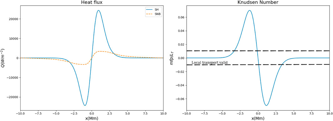
FIGURE 1. Left: Heat flux from the Spitzer–Harm model and the SNB flux for the same temperature profile. Right: The Knudsen number for this temperature profile. The dashed lines indicate the band where the magnitude of the Knudsen number is $<0.01$. A local model for heat flow is not valid outside of this band.

During the expansion and ordering procedures for deriving the SNB model, the electric field, a function of the perturbed distribution function and, therefore, the source of non-linearity, is dropped from the SNB equivalent of Eq. 4. Its effect is phenomenologically re-introduced as a correction factor in the mean-free path λ′. In the original SNB model, the electric field is the local Spitzer–Harm electric field $\mathit{E}=k_{\text{B}}{T}_{\text{e}}\left(\nabla \log n_{\text{e}}+1.7\nabla \log T_{\text{e}}\right)$. More recent studies have shown that this electric field term has little effect and is, therefore, usually omitted. It is kept here, as it may be that turbulent scattering affects thermal conduction (Bian et al., 2016). This effective reduction of the mean-free path may be included in the SNB model in a similar way to the electric field correction mentioned above. Another limitation of SNB is that since it is based on an expansion of the distribution function to first order, (f = f₀ + f₁), it is unlikely to be a good approximation for K_n > 1 when the assumption is that f_M > f₁ will be violated. The precise upper limit on the Knudsen number for SNB to be valid in the solar corona is as of yet unknown. Certainly, however, for K_n ≫ 1, alternative models must be used for the high-energy electrons.

In laser–plasma, the SNB model has been compared against other non-local models and VFP in the study by Brodrick et al. (2017) and for inertial fusion in the study by Sherlock et al. (2017). These showed that SNB can accurately predict non-local heat fluxes even when the distribution is not close to the VFP distribution. This suggests a level of robustness in finding heat fluxes even for distributions far from the Maxwellian ones, but as of yet, this has not been tested for solar coronal problems. It should be noted that there is an alternative approach based on solving the VFP equation for the high-velocity part of only the distribution function (Ljepojevic & Burgess, 1990). A comparison of this model to SNB would be informative.

6 Conclusion

Classical thermal conduction in plasmas requires that the plasma is collision-dominated. The key step in this derivation is that the mean-free path of the electrons carrying the majority of the heat must be less than the temperature scale length. Since the mean-free path scales as v⁴ and the heat is primarily carried by electrons with speeds between 2.5 and 3.5 v_T, this means that local transport models fail when the Knudsen number is greater than 0.01. This condition will be easily satisfied in the solar atmosphere.

The two effects of non-local transport are that the thermal flux becomes limited and there is preheat associated with high energy, and least collisional component of the electron distribution function. The first of these can be accounted for by applying a flux limiter. However, this has to be tuned to match the observations, and it is problem-dependent and cannot capture preheat. Kernel-based non-local models, such as LMV, can simulate both flux limiting and preheat, but they are dependent on the choice of the kernel function, require some arbitrary tuning parameters, and are computationally expensive in 3D. The expense is because the method must solve along field lines, requiring many field lines to be traced, and LMV should also be solved along each of them.

Recent advances in the modelling of laser–plasmas, mostly motivated by fusion research studies, have led to the development of the non-local SNB model. This has the advantage, compared to LMV, of being solved using corrections to local fluxes, hence not requiring integration along the field lines. This makes SNB more computationally efficient than LMV. SNB has also been extensively tested against VFP codes, where it has been shown to accurately capture preheat and flux limiting without having to tune free parameters. Based on the review, in this article, it is clear that for active region solar atmospheres, there is little justification for using Spitzer–Harm conductivity in the MHD theory. The minimum model required is a flux limiter, but for the highest fidelity solution for thermal transport, SNB is recommended.

Author contributions

TA wrote the majority of the manuscript. TG completed the basic SNB analysis for Figure 1, solving the SNB equations. CR updated and checked the SNB theory.

Conflict of interest

The authors declare that the research was conducted in the absence of any commercial or financial relationships that could be construed as a potential conflict of interest.

Publisher’s note

All claims expressed in this article are solely those of the authors and do not necessarily represent those of their affiliated organizations, or those of the publisher, the editors and the reviewers. Any product that may be evaluated in this article, or claim that may be made by its manufacturer, is not guaranteed or endorsed by the publisher.

References

Bian, N. H., Kontar, E. P., and Emslie, A. G. (2016). Suppression of parallel transport in turbulent magnetized plasmas and its impact on the NON-thermal and thermal aspects of solar flares. Astrophysical J. 824, 78. doi:10.3847/0004-637X/824/2/78

CrossRef Full Text | Google Scholar

Brodrick, J. P., Kingham, R. J., Marinak, M. M., Patel, M. V., Chankin, A. V., Omotani, J. T., et al. (2017). Testing nonlocal models of electron thermal conduction for magnetic and inertial confinement fusion applications. Phys. Plasmas 24, 092309. doi:10.1063/1.5001079

CrossRef Full Text | Google Scholar

Cheung, M. C. M., Rempel, M., Chintzoglou, G., Chen, F., Testa, P., Martínez-Sykora, J., et al. (2019). A comprehensive three-dimensional radiative magnetohydrodynamic simulation of a solar flare. Nat. Astron 3, 160–166. doi:10.1038/s41550-018-0629-3

CrossRef Full Text | Google Scholar

Del Sorbo, D., Feugeas, J. L., Nicolaï, P., Olazabal-Loumé, M., Dubroca, B., Guisset, S., et al. (2015). Reduced entropic model for studies of multidimensional nonlocal transport in high-energy-density plasmas. Phys. Plasmas 22, 082706. doi:10.1063/1.4926824

CrossRef Full Text | Google Scholar

Farmer, W. A., Jones, O. S., Barrios, M. A., Strozzi, D. J., Koning, J. M., Kerbel, G. D., et al. (2018). Heat transport modeling of the dot spectroscopy platform on NIF. Plasma Phys. Control. Fusion 60, 044009. doi:10.1088/1361-6587/aaaefd

CrossRef Full Text | Google Scholar

Fundamenski, W. (2005). Parallel heat flux limits in the tokamak scrape-off layer. Plasma Phys. Control. Fusion 47, R163–R208. doi:10.1088/0741-3335/47/11/R01

CrossRef Full Text | Google Scholar

Jones, O. S., Suter, L. J., Scott, H. A., Barrios, M. A., Farmer, W. A., Hansen, S. B., et al. (2017). Progress towards a more predictive model for hohlraum radiation drive and symmetry. Phys. Plasmas 24 (5), 056312. doi:10.1063/1.4982693

PubMed Abstract | CrossRef Full Text | Google Scholar

Karpen, J. T., and Devore, C. R. (1987). Nonlocal thermal transport in solar flares. Astrophys. J. 320, 904. doi:10.1086/165608

CrossRef Full Text | Google Scholar

Ljepojevic, N. N., and Burgess, A. (1990). Calculation of the electron velocity distribution function in a plasma slab with large temperature and density gradients. Proc. R. Soc. A. doi:10.1098/rspa.1990.0026

CrossRef Full Text | Google Scholar

Luciani, J. P., Mora, P., and Virmont, J. (1983). Nonlocal heat transport due to steep temperature gradients. Phys. Rev. Lett. 51, 1664–1667. doi:10.1103/PhysRevLett.51.1664

CrossRef Full Text | Google Scholar

Marocchino, A., Tzoufras, M., Atzeni, S., Schiavi, A., Nicolaï, P. D., Mallet, J., et al. (2013). Comparison for non-local hydrodynamic thermal conduction models. Phys. Plasmas 20, 022702. doi:10.1063/1.4789878

CrossRef Full Text | Google Scholar

Omotani, J. T., and Dudson, B. D. (2013). Plasma Physics and controlled fusion. doi:10.1088/0741-3335/55/5/05500

CrossRef Full Text | Google Scholar

Schurtz, G. P., Nicolai, P., and Busquet, M. (2000). A nonlocal electron conduction model for multidimensional radiation hydrodynamics codes. Phys. Plasmas 7, 4238. doi:10.1063/1.1289512

CrossRef Full Text | Google Scholar

Sherlock, M., Brodrick, J. P., and Ridgers, C. P. (2017). A comparison of non-local electron transport models for laser-plasmas relevant to inertial confinement fusion. Phys. Plasmas 24. doi:10.1063/1.4986095

CrossRef Full Text | Google Scholar

Silva, S., Santos, J. C., Büchner, J., and Alves, M. V. (2018). Nonlocal heat flux effects on temperature evolution of the solar atmosphere. Astronomy Astrophysics 615, A32. doi:10.1051/0004-6361/201730580

CrossRef Full Text | Google Scholar

Spitzer, L., and Härm, R. (1953). Transport phenomena in a completely ionized gas. Phys. Rev. 89, 977–981. doi:10.1103/physrev.89.977

CrossRef Full Text | Google Scholar

van der Holst, B., Sokolov, I. V., Meng, X., Jin, M., Manchester, B. W., Tóth, G., et al. (2014). ALFVÉN WAVE SOLAR MODEL (AWSoM): Coronal heating. Astrophysical J. 782, 81. doi:10.1088/0004-637X/782/2/81

CrossRef Full Text | Google Scholar

Wang, T., Ofman, L., Sun, X., Solanki, S. K., and Davila, J. M. (2018). Effect of transport coefficients on excitation of flare-induced standing slow-mode waves in coronal loops. Astrophysical J. 860, 107. doi:10.3847/1538-4357/aac38a

CrossRef Full Text | Google Scholar

West, M. J., Cargill, P. J., and Bradshaw, S. J. (2004). SOHO-15. ESA Publications, 573–576.

Google Scholar

Wigram, M. R. K., Ridgers, C., Dudson, B., Brodrick, J., and Omotani, J. (2020). Incorporating nonlocal parallel thermal transport in 1D ITER SOL modelling. Nucl. Fusion 60, 076008. doi:10.1088/1741-4326/ab868b

CrossRef Full Text | Google Scholar