Solar-induced 27-day modulation on polar mesospheric cloud (PMC), based on combined observations from SOFIE and MLS

1 Introduction

The polar mesospheric cloud (PMC) is formed in the mesopause region (80–90 km) over the high latitude (>50°) during summer times (Hervig et al., 2012). PMCs are mainly composed of small water ice crystals (having a radius of about 30–100 nm), which can effectively scatter sunlight to make it visible from the ground after dusk and before dawn (Hervig et al., 2012; Dalin et al., 2018). The extremely low temperatures (T < 140 K) at the summer mesopause, accompanied by increased water vapor content, result in a supersaturated state for the formation of water ice aerosols (Hervig et al., 2001). In the northern hemisphere (NH), a typical PMC season lasts from late May to the end of August (Gadsden, 1981), while PMCs appear from late November to mid-February in the southern hemisphere (SH) (Ludlam, 1976; Thomas, 1985).

PMCs are very sensitive to changes in the mesopause environment and are influenced by many atmospheric parameters, such as temperature (Thomas et al., 2015), water vapor content (Thomas et al., 2015), gravity waves (Gerrard et al., 2004; Chandran et al., 2010), planetary waves (Merkel et al., 2003; von Savigny et al., 2007), and interhemispheric coupling (Karlsson et al., 2007; Karlsson et al., 2009). Therefore, PMCs are considered an important indicator of mesospheric state.

Solar activity and its variations can affect PMCs by affecting the temperature and water vapor in the summer mesopause (Hervig and Siskind, 2006). Due to the solar activities manifested from sunspots, plages, faculae, and eruptive flares, the solar radiation received by Earth is quasi-periodic, with the main period of 27 days (e.g., roughly the Carrington solar rotation period), or weaker periodic modulation of 13 days and 9 days (Lean and Repoff, 1987; Velasco Herrera et al., 2022). This 27-day periodic modulation with radiation and charged particle bursts affects the radiative photochemical and kinetic state of Earth’s mesosphere (Hood et al., 1991; Beig et al., 2008).

Observations from satellites and ground-based instruments show that the frequency of occurrence (Robert et al., 2010; von Savigny et al., 2013b), albedo (von Savigny et al., 2013b), ice water content (Thurairajah et al., 2017), and brightness (Dalin et al., 2018) of PMCs are characterized by a 27-day periodicity. This period has been proposed to be physically connected with the solar $Lyman–\alpha$ flux with a time lag of 0–1 day (Robert et al., 2010; von Savigny et al., 2013a; Thurairajah et al., 2017; Dalin et al., 2018). The solar $X-ray$, EUV, and UV irradiance can influence the ozone concentration through reactions of O₂ → O + O and O₂ + O → O₃ (Arnold and Comes, 1979). The source of heat between 50 and 100 km atm is mainly from absorption of solar radiation and the exothermic heat from chemical reactions (Mlynczak, 1996). The process involving ozone can provide up to 80% of the heat budget (Mlynczak, 1996). In the range of ∼80–100 km, the response of ozone and temperature to solar changes at all latitudes is positive with consistent phases (Huang et al., 2016). Therefore, enhanced solar irradiance and ozone concentration will affect the mesospheric temperature through the radiative heating rate and chemical heating rate of ozone (Robert et al., 2010). Thus, the local and regional temperatures may remain above the freezing point with large-enough heating energy source from the Sun (Robert et al., 2010; von Savigny et al., 2013b). During the same time, the available solar radiation can also photolyze water vapor, preventing or weakening the formation of PMCs (Robert et al., 2010; von Savigny et al., 2013a). Simulation of the effects of 27-day solar ultraviolet forcing on the mesospheric temperature shows that the 27-day solar rotational modulation cycle is intermittent, and its influence may further depend on atmospheric dynamics (Gruzdev et al., 2009).

The superposed epoch analysis (SEA) can extract signals of PMCs in response to solar activity forcing beyond the background noise; e.g., the data can be properly averaged to amplify the useful signals by eliminating any background noise (e.g., Robert et al., 2010; Thomas et al., 2015). Using this method, the response of temperature and water vapor to solar irradiance variations (with a primary period of 27 days) measured by the SOFIE onboard the Aeronomy of Ice in the Mesosphere (AIM) is within 0–8 days and 0–3 days, respectively, both of which are shorter than the expected time for direct solar heating and photodissociation (Thomas et al., 2015). Based on the long-term data set from ground observations, the average lag time of PMC brightness to solar $Lyman-\alpha$ flux is 0–3 days (Dalin et al., 2018). Since the theoretical photochemical lifetime of mesopause water vapor is about 5–10 days, direct solar heating and atmospheric dynamical processes play a dominant role in PMC brightness variation (Dalin et al., 2018).

In this research, the IWC and temperature measured by the SOFIE and additional mesospheric temperature observations from the Microwave Limb Sounder (MLS) onboard the Aura satellite are co-analyzed. The solar activity index, Y10, which includes both $X-ray$ and $Lyman-\alpha$ (Tobiska, 2010) is adopted. Combined with Y10, the SEA is used to extract the time lag of IWC and temperature in response to solar activity forcing over the NH and SH, respectively. In addition, the cross-correlation curves between the average temperature and solar forcing for different atmospheric pressures and latitudes of the PMC seasons from 2004 to 2020 are also compared and analyzed. The data processing methods are presented in Section 2. Section 3 introduces the data used in this study. Section 4 gives the results and explanations. Finally, Section 5 summarizes the study.

2 Data and method

2.1 Measurements and data pre-processing

The SOFIE is one of the three scientific instruments onboard AIM, which is dedicated to the study of PMCs and their formation environment for the first time (Gordley et al., 2009). A detailed description of the SOFIE instrument can be found in Gordley et al. (2009). It measures the reduction of solar intensity when light passes through an atmospheric tangent path at sunset or sunrise from orbit, based on the solar occultation method. The SOFIE provides 15 sunrise measurements from ∼60° to 85°S and 15 sunset measurements from ∼60° to 85°N per day, essentially after the day–night terminator. The SOFIE field-of-view (FOV) subtends ∼1.6 km vertically, and the detectors are oversampled at ∼0.2-km intervals. We use version 1.3 temperature and IWC data available from the SOFIE website (http://gats-inc.com).

The Microwave Limb Sounder (MLS), carried on the Aura satellite and launched on 15 July 2004, measures the thermal microwaves of atmospheric substances by five spectra from 115 GHz to 2.5 THz through limb observation (Waters et al., 2006). The MLS scans vertically with spatial coverage of a nearly global scale (with the latitude of −82° to +82°) (Waters et al., 2006). Each profile is 1.5° in latitude or 165 km along the orbit (e.g., approximately 15 orbits per day), with vertical coverage ranging from 0.0010 Pa to 100,000 Pa (Schwartz et al., 2008). The vertical scan rate varies with altitude and is faster in the upper atmosphere, resulting in poor vertical resolution in the mesosphere (Robert et al., 2010). Therefore, only the temperature data at 0.1 Pa, 0.22 Pa, and 0.46 Pa are utilized in this study. We have used version 5.0 temperature data from https://aura.gsfc.nasa.gov/science/data.html.

In order to analyze the correlation between the 27-day modulation of solar Y10 index and PMC variations, the time series of Y10, mesospheric temperature, and the IWC have to be properly prepared. The variation of solar radiation intensity causes fluctuations of temperature and IWC above and beyond the background values. According to previous studies, a 35-day window can be used for the smoothing filter, which removes stochastic variability and random noise (Hood et al., 1991; Robert et al., 2010; Thomas et al., 2015). Then, the time series of the anomalies caused by the variation of solar radiation can be obtained by subtracting the running mean of 35 days from the original time series (e.g., Hood et al., 1991; Robert et al., 2010; Thomas et al., 2015). After the smoothing step to remove background noises, we further use a 5-day running mean to smooth the anomalous time series. Since the smoothing process causes the same phase shift in all three data sets: temperature, IWC, and Y10, the effect of smoothing on the results of the following correlation analyses should be almost negligible.

An example of smoothing of Y10 during the 2008 PMC season of the NH is shown in Figure 1A. Figure 1B plots the average temperature in the latitude range of ∼60°–80° at 0.46 Pa (about 84 km altitude) atmospheric pressure from the MLS. Figure 1C shows the anomaly curves of Y10 and temperature relative to solstice days, and there is a delayed change in the temperature anomaly. Figure 1D shows the correlation coefficient of Y10 and temperature anomalies in different time lag days. The time lag days corresponding to the two peaks of the correlation curve are 23 days and 4 days, respectively, with the duration of the time interval equal to $\left|-23\right|+4=27$. The periodic variations reveal that there are 27-day characteristics of the solar cycle in the mesospheric temperature data set, which is consistent with previous results (e.g., Robert et al., 2010).

FIGURE 1

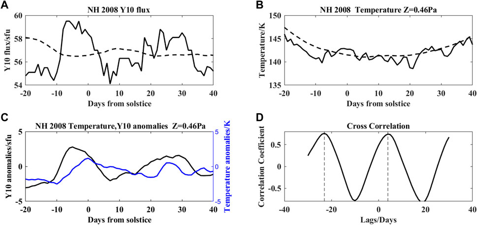
FIGURE 1. (A) Solar radiation index Y10 (solid line) and its 35-day running mean (dotted line) during the NH PMC season in 2008. (B) Average temperature (solid line) and its 35-day running mean (dotted line) in the latitude range of ∼60°–80° at 0.46 Pa atmospheric pressure during the 2008 NH PMC season. (C) Y10 anomaly (black line) and temperature anomaly (blue line) to relative summer solstice days. (D) Correlation coefficient between Y10 anomaly and temperature anomaly at different time lags.

2.2 Cross-correlation analysis and significance test

The Spearman's rank correlation coefficient is stable and insensitive to noise. Any two variables $x$ and $y$ will be sorted according to their sizes, with the sample number $n$. The sorted serial numbers are denoted as $D_x^i$ and $D_y^i$, respectively. Then, the Pearson correlation coefficient between the new sequence is the Spearman rank correlation coefficient ($r_s$) (Spearman, 2010), given as

${\mathit{r}}_{\mathit{s}}\left(\mathit{x},\mathit{y}\right)=\frac{{\displaystyle \sum _{\mathit{i}=\mathbf{1}}^{\mathit{n}}}\left({\mathit{D}}_{\mathit{x}}^{\mathit{i}}-\overline{{\mathit{D}}_{\mathit{x}}}\right)\left({\mathit{D}}_{\mathit{y}}^{\mathit{i}}-\overline{{\mathit{D}}_{\mathit{y}}}\right)}{\sqrt{{\displaystyle \sum _{\mathit{i}=\mathbf{1}}^{\mathit{n}}}{\left({\mathit{D}}_{\mathit{x}}^{\mathit{i}}-\overline{{\mathit{D}}_{\mathit{x}}}\right)}^{\mathbf{2}}{\displaystyle \sum _{\mathit{i}=\mathbf{1}}^{\mathit{n}}}{\left({\mathit{D}}_{\mathit{y}}^{\mathit{i}}-\overline{{\mathit{D}}_{\mathit{y}}}\right)}^{\mathbf{2}}}},(1)$

and simplified to

${\mathit{r}}_{\mathit{s}}\left(\mathit{x},\mathit{y}\right)=\mathbf{1}-\frac{\mathbf{6}{\displaystyle \sum _{\mathit{i}=\mathbf{1}}^{\mathit{n}}}{\left({\mathit{D}}_{\mathit{x}}^{\mathit{i}}-{\mathit{D}}_{\mathit{y}}^{\mathit{i}}\right)}^{\mathbf{2}}}{\mathit{n}\left({\mathit{n}}^{\mathbf{2}}-\mathbf{1}\right)}$(2).

In one PMC season, the selected time series of mesospheric temperature anomalies is

$\mathit{D}\mathit{T}\left({\mathit{d}\mathit{a}\mathit{y}}_{\mathbf{1}},\dots \dots .,{\mathit{d}\mathit{a}\mathit{y}}_{\mathit{n}}\right)$(3).

When the delay-day parameter is set as lags, the corresponding time series of Y10 anomalies will be

$\mathit{D}\mathit{Y}\mathbf{10}\left({\mathit{d}\mathit{a}\mathit{y}}_{\mathbf{1}}-\mathit{l}\mathit{a}\mathit{g}\mathit{s},\dots \dots .,{\mathit{d}\mathit{a}\mathit{y}}_{\mathit{n}}-\mathit{l}\mathit{a}\mathit{g}\mathit{s}\right)$(4).

Then, their rank correlation coefficient is $\left.r_s\left(DT,DY10\right)\right)$ for the time lag correlation analysis.

The significance of the rank correlation coefficient can be tested using the Z statistic, which is calculated as

$\mathit{Z}=\frac{{\mathit{r}}_{\mathit{s}}}{\sqrt{\mathbf{1}/\left(\mathit{n}-\mathbf{1}\right)}}.(5)$

In this study, we cover the data from 20 days before the summer solstice to 40 days after the solstice, with a data length of n = 61 days. When the significant level is 0.05, then $Z=1.65$ from the Supplementary Table A1. When the data length $n=61$, $r_s=0.21$ is calculated. Therefore, when the calculated rank correlation coefficient is higher than 0.21, the significance level can be higher than 95%.

2.1 Superposed epoch analysis

The superposed epoch analysis (SEA) can extract the response signal under certain forcing that is different from the random noise (Chree, 1913), and this method is widely used to study the response of PMCs to the 27-day solar forcing (e.g., Robert et al., 2010; Thomas et al., 2015). A distinct 27-day signal is selected from the Y10 anomaly time series. The maximum/peak of this signal is then identified as a key date or day 0 and the 35-day time series starting from day 0 is used for the study from the PMCs season. The Y10 anomalies of different seasons are arranged together by rows and then averaged by columns to obtain a single 35-day Y10 anomaly time series (e.g., super-forcing function). Similarly, executing the same process for the temperature and IWC on the corresponding dates will yield two super-response functions. By averaging, the noise in the data will be much reduced because random noise tends to cancel each other out. Table 1 shows the PMC seasons and the key dates of the selected PMC seasons used for the SEA in this study. Some seasons have no obvious 27-day period of Y10 anomalies, so those seasons are excluded for the SEA (marked with asterisks in Table 1).

TABLE 1

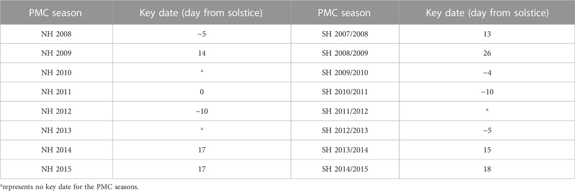
TABLE 1. Key dates of the selected PMC seasons used for the SEA.

3 Data processing

3.1 Solar activity index and PMCs indicator

The Y10, which includes both $X-ray$ and $Lyman-\alpha$, is selected as the index of solar activity (Tobiska, 2010). The $X-ray$ covers the wavelength ranges between 0.1 and 0.8 nm and comes from the cold and hot parts of the solar corona, usually combined with the very bright and slowly changing solar activity region (with a time scale of days to months) and rapidly varying flares (minutes to hours) (Tobiska et al., 2008). Its photons reaching Earth are absorbed by molecular oxygen ($O_2$) and molecular nitrogen ($N_2$) at the upper mesosphere and lower thermosphere (MLT, e.g., 70–90 km) (Nicolet and Aikin, 1960). They can ionize the neutral components and create the D region of the ionosphere (Thomson et al., 2004). The $Lyman-\alpha$ is produced in the upper chromosphere and transition region of the Sun (Woods and Rottman, 1997). It is mainly formed in the solar active area and flocculus (Woods and Rottman, 1997). It is also absorbed in the MLT region, decomposing $NO$ (Woods and Rottman, 1997) and participating in the chemical reaction of $H_{2}O$ (Frederick, 1977). The Y10 is obtained by weighting the $X-ray$ and $Lyman-\alpha$ without the flare component (Tobiska, 2010). During high solar activity, the main energy source of the MLT is the $X-ray$ radiation, while during moderate and low solar activities, it is the $Lyman-\alpha$ radiation (Tobiska, 2010). For the intermediate phase between the maximum and minimum of the 11-year-like sunspot and solar activity cycles, the $X-ray$ and $Lyman-\alpha$ are competitive in the MLT region.

We investigate the influence of solar radiation on PMCs in two steps. The first step is to study the response of mesopause temperature and IWC to the 27-day periodic variation of Y10. The second step studies the response of IWC to temperature variation, linking the effect of solar radiation on PMCs through temperature to IWC. As mentioned above, PMCs are affected by different atmospheric physical processes, many of which are not directly related to solar radiation. Therefore, appropriate parameters must be filtered out as indicators of PMC properties. Since PMCs are mostly composed of small ice crystals, the IWC data collected by the SOFIE in the nine NH PMC seasons (from 2007 to 2015) and eight SH PMC seasons (from SH 2007/2008 to 2014/2015) are processed as the index. The variations of the IWC can directly reflect the nature of the PMCs. The data from 30 days before and after the summer solstice are selected for each PMC season when supersaturation occurs and the water vapor can condense into ice particles to form PMCs.

3.2 Temperature data over the mesopause

The temperature is considered to be the main driving factor of the 27-day periodic variation of PMCs (Robert et al., 2010; von Savigny et al., 2013b). Microphysical model results reveal that the mass density of the PMCs is weakly dependent on the abundance of condensation nuclei (Megner, 2011). According to the previous study, ice particles will condense and grow when the saturation vapor pressure $\left(S\right)$ is greater than 1 (Thomas, 1996). The calculation of $S$ is given as follows:

$S=\frac{w\left(H_{2}O\right)\times p}{e^{\left(28.548-\left(6077.4÷T\right)\right.}}=\frac{e^{\left(6077.4÷T\right)}}{e^{\left(28.548\right)}}\times w\left(H_{2}O\right)\times p,(6)$

where $p$ is the total gas pressure in $hPa$, and $w\left(H_{2}O\right)$ is the water vapor mixing ratio (Thomas, 1996). The denominator in Eq. 6 is the saturation vapor pressure according to Marti and Mauersberger (1993).

From Eq. 6, we can see that $S$ is exponentially related to temperature but linearly related to water vapor. The summer mesopause temperature is often lower than 140 K (Hervig et al., 2001) according to the observed data. Therefore, in order to simplify the relationship between PMCs and solar activity, the effect of water vapor can be ignored, and only the temperature is chosen as the intermediate variable. Based on the observed data from MLS during 2004–2020, the response of the mesospheric temperature to the solar radiation at 0.46 Pa pressure height (e.g., about 84 km) is analyzed for both the NH and SH PMC seasons. The variation of response over different altitudes at 0.1 Pa, 0.22 Pa, and 0.46 Pa (80–90 km) is also studied.

4 Results and discussions

4.1 Analysis of SEA results

It is assumed that the response follows the peak forcing and the time lag is always positive (Thomas et al., 2015). According to previous results, solar forcing is positively correlated with temperature (Thomas et al., 2015; Köhnke et al., 2018) and negatively correlated with IWC (Thurairajah et al., 2017). The cross-correlation between Y10 and temperature anomalies can act as a function of time lag. The time lags corresponding to the peaks of the correlation curves are the time required for the temperature to respond to the solar forcing. For the IWC, the time lags corresponding to the troughs of the correlation curves are the time required for the IWC to respond to the solar forcing.

Figure 2 shows the average response of temperature anomalies from the SOFIE and MLS to solar forcing for both hemispheres. The results reveal that the time lags with statistical significance >95% of the NH temperature response to Y10 are 2 days (based on the data from the SOFIE) and 1 day (for the MLS data set). While in the SH, the time lag days are 12 days (for SOFIE and MLS). With significant differences, the time lags in the SH are much longer than those in the NH.

FIGURE 2

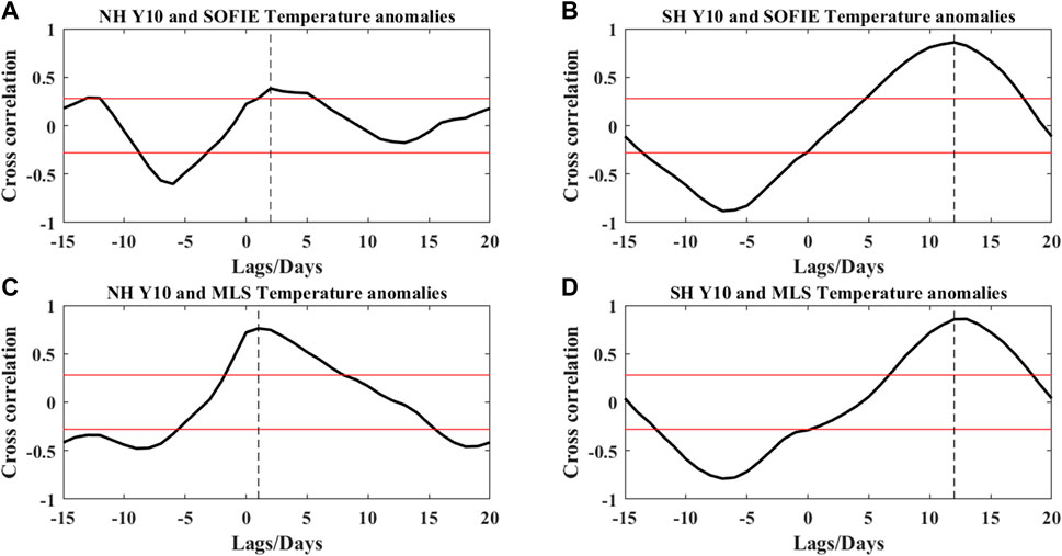
FIGURE 2. (A) Correlation curve of temperature anomaly from SOFIE and Y10 anomaly in the NH calculated through SEA. (B) Correlation curve of SOFIE temperature anomaly and Y10 anomaly in the SH. (C) Correlation curve of temperature anomaly from MLS and Y10 anomaly in the NH. (D) Correlation curve of MLS temperature anomaly and Y10 anomaly in the SH. Red lines correspond to the correlation coefficients with statistical significance equal to 95%.

Figure 3 exhibits the average response of the IWC to solar forcing for the NH (left) and SH (right). The time lags in the NH are 2 days (with a statistical significance of >95% of all days), and the time lags in the SH are 14 days. The trough in the NH is lower than that in the SH, indicating that the statistical significance is higher in the NH. Previous results have shown that the IWC anomalies are negatively correlated with 0–5 days in the NH and 3–8 days in the SH (Thurairajah et al., 2017). By contrast, our results are closer to those in the NH but larger than those in the SH. The SEA reveals that the relationship between IWC and Y10 shows a delayed response between the PMCs and solar activity, with longer time lags in the SH than in the NH. In the region of 70–90 km during the PMC seasons, the temperature time lag caused by $Lyman-\alpha$ heating is theoretically calculated to be about 4 days, independent with altitude (Thomas et al., 2015). It follows that the time lag (2 days) of the temperature response to solar forcing in the NH is likely to be caused by direct solar heating, while the time lag of 12 days in the SH is still uncertain. Since the 27-day period of solar variability and its harmonics is close to the typical period of wave-like disturbances occurring in the middle atmosphere (Gruzdev et al., 2009), the atmospheric dynamical effects, such as the 27-day vertical wind oscillations, could possibly overlap the effects of solar forcing on temperature (Ebel et al., 1986). Thus, the abnormal temperature response time for the SH occurs.

FIGURE 3

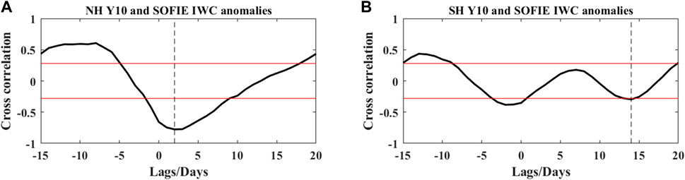
FIGURE 3. (A) Correlation curve between IWC anomaly and Y10 anomaly in the NH calculated by SEA. (B) Correlation curve in the SH. Red lines correspond to the correlation coefficients with statistical significance equal to 95%.

The average response of IWC to temperature in the NH versus SH is shown in Figure 4. The delay days corresponding to the trough are the time lags of the response of IWC to temperature anomalies. The trough below the red line indicates that the statistical significance is >95%. The time lag in the NH is always 0 days, as shown in Figures 4A, C. In the SH, the time lag is 1 day (shown in Figure 4D, based on data from the MLS, with a statistical significance of >95%) and −1 day (shown in Figure 4B, based on data from the SOFIE with statistical insignificance). The result indicates that when the temperature changes in the NH, the IWC can respond rapidly, and the average time lag is 0 days. Due to the limitation of the temporal resolution of the observed data, we can only study the response of IWC and mesosphere temperature to Y10 in days. If the time lag day for the response of IWC to the mesosphere temperature is 0 day. Therefore, the temperature anomaly in the NH can directly reflect the PMC activity. Temperature connects solar forcing with PMCs through the impacts of temperature variations on the properties of the PMCs synchronously. By contrast, the IWC in the SH is less sensitive to the temperature anomaly, with a time lag of 1 day.

FIGURE 4

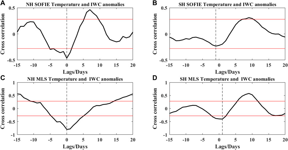
FIGURE 4. (A) Correlation curve of SOFIE temperature anomaly and IWC anomaly in the NH calculated by SEA. (B) Correlation curve of SOFIE temperature anomaly and IWC anomaly in the SH. (C) Correlation curve between MLS temperature anomaly and IWC anomaly in the NH. (D) Correlation curve between MLS temperature anomaly and IWC anomaly in the SH. Red lines correspond to the correlation coefficients with statistical significance equal to 95%.

4.2 Further study on effect of Y10 on mesospheric temperature

4.2.1 Comparison of time lag at different latitudes

Figures 5, 6 show the correlation between Y10 and temperature anomalies at different latitudes in the NH and SH during the PMC seasons from 2004 to 2020 at 0.46 Pa pressure height. The Y10 anomalous signals or temperature anomalies with no 27-day periodicity shows irregularity in the results of the correlation analysis (e.g., for the PMC season of NH 2010 in Figure 5). From Figures 5, 6, it can be found that only two PMC seasons (e.g., NH 2008 and NH 2012) have a time lag of 0–5 days (depending on the latitude), which is close to the time lag of direct heating by solar radiation with 4 days. Therefore, the temperature changes in these two PMC seasons are likely to be caused by solar forcing. At the same time, the time lag of temperature in these two PMC seasons shows an increasing trend from the low latitudes to the pole. Therefore, we can find that the low latitudes are more sensitive to solar activity with a faster response time, while the high latitude area has weak sensitivity to solar activity with a longer response time. Our result is consistent with previous studies; e.g., Gruzdev et al. (2009) have found that the sensitivity of mesospheric temperature to solar activity usually decreases with the latitude when using a three-dimensional chemical climate model.

FIGURE 5

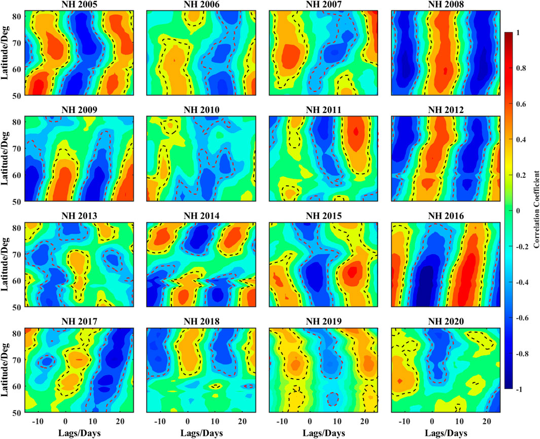
FIGURE 5. Correlation between the temperature and Y10 anomalies at 0.46 Pa over different latitudes, for the NH PMCs seasons during 2005–2020. The temperature data from MLS is averaged in the corresponding latitude. The red area surrounded by black dashed lines indicates that the significance level of the positive correlation between temperature and Y10 is greater than 95%. The blue area surrounded by the red dotted line indicates that the significance level of the negative correlation between temperature and Y10 is greater than 95%.

FIGURE 6

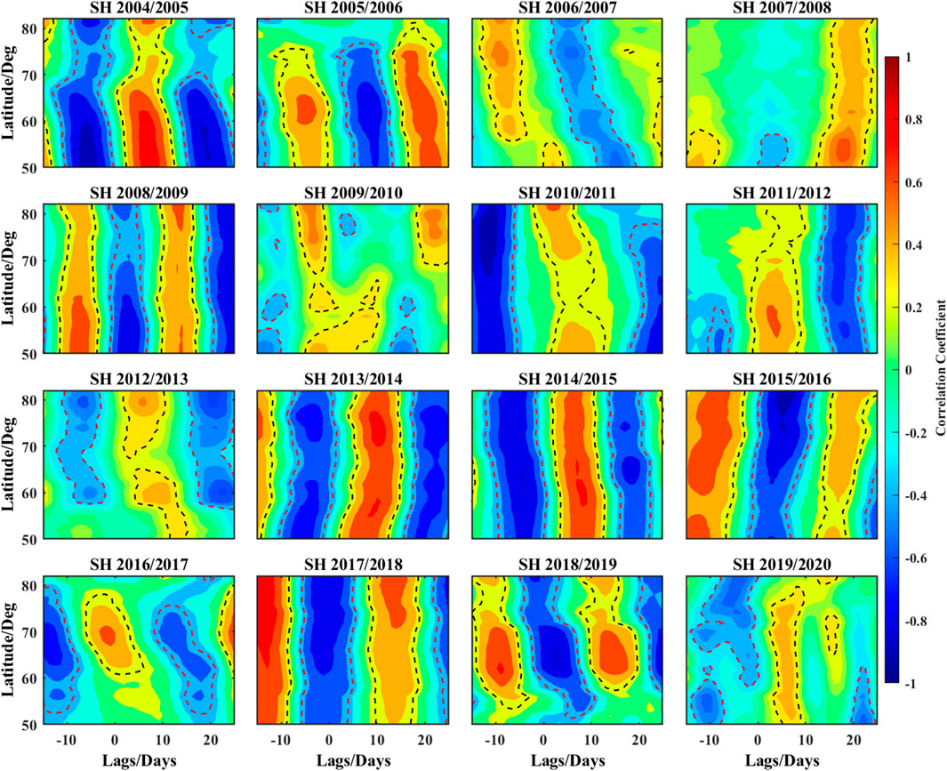
FIGURE 6. Correlation between the temperature and Y10 anomalies at 0.46 Pa over different latitudes, for the SH PMCs seasons during 2005–2020. The temperature data from MLS is averaged in the corresponding latitude. The red area surrounded by black dashed lines indicates that the significance level of the positive correlation between temperature and Y10 is greater than 95%. The blue area surrounded by the red dotted line indicates that the significance level of the negative correlation between temperature and Y10 is greater than 95%.

For the PMC seasons with a long temperature delay (time lag >5 days) but obvious 27-day period of temperature anomaly, the mesopause temperature could probably be modulated by the dynamic effect of the 27-day period. According to Figures 5, 6, we can classify two types of PMC seasons with distinct characteristics: one is NH 2016 and SH 2015/2016, whose temperature time lag increases with increasing latitude; the other is SH 2008/2009, SH 2014/2015, and SH 2017/2018, whose temperature delay is almost equal at different latitudes. Therefore, it indicates there are two different 27-day atmospheric dynamical modulation mechanisms at the mesopause.

Meanwhile, it is found from both Figures 5, 6 that there is an anticorrelation between temperature and Y10 at a time lag of 10 days in NH 2005 and NH 2016, which are PMC seasons that are 11 years apart. Similarly, in SH 2004/2005 and SH 2014/2015 in the 50°–70° latitude range, there is a positive correlation between temperature and Y10 near the time lag of 10 days and a negative correlation near the time lag of −5 days and 20 days. These two PMC seasons are also 11 years apart. It is therefore indicated that these characteristics in the PMC seasons may be related to possible modulation by the 11year solar cycle.

4.2.2 Comparison of time lag days at different atmospheric pressure levels

We selected 12 PMC seasons with obvious 27-day periodicity and compared the average time lag of the average temperature in the latitude range of 53°–81° from the MLS at three different atmospheric pressures (e.g., 0.10 Pa, 0.22 Pa, and 0.46 Pa); the statistical results are summarized in Table 2. Among them, 9/12 cases have a distinct pattern of increasing time lags with increasing atmospheric pressure (decreasing altitude); that is, the lower the altitude, the longer the time lags. These cases are marked in bold in Table 2, which are PMC seasons of NH 2009, NH 2016, NH 2019, SH 2005/2006, SH 2008/2009, SH 2013/2014, SH 2014/2015, SH 2015/2016, and SH 2017/2018. From the temperature time lag (>5 days), we can infer that this pattern is caused by the dynamic forcing of the atmosphere. This dynamic disturbance mechanism will probably first cause the temperature change in high altitudes. It is assumed that the dynamic forcing is caused by a 27-day period of vertical wind oscillation (Ebel et al., 1986). When the wind direction propagates down, the adiabatic warming (Jenssen and Radok, 1964) first causes temperature disturbances at high altitudes. This modulation mechanism is consistent with our results.

TABLE 2

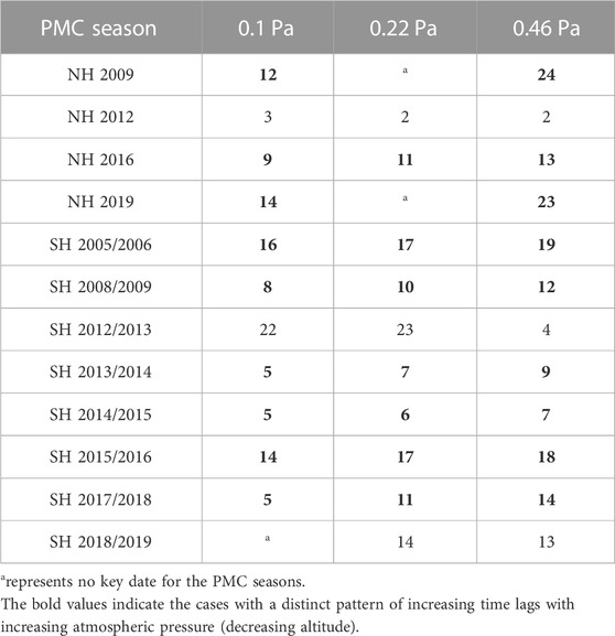
TABLE 2. Average time lag (in days) of temperature response to the 27-day solar rotational modulation in the latitude range 53°–81° at different atmospheric pressure values.

5 Conclusion

In this research, we study the impact of activity and variability of solar radiation on the polar mesospheric clouds (PMCs) based on the correlations between the composite solar index Y10, the mesospheric temperature, and the ice water content (IWC). Surprisingly, this is the first time that Y10 has been used as an index of solar activity to study PMCs. We analyze the response of IWC to the mesospheric temperature and Y10 anomalies, respectively, through the superposed epoch analysis (SEA) method. It is found that when the temperature anomaly changes in response to the 27-day solar modulation, the IWC can respond rapidly, with an average response time lag of 0 days in the northern hemisphere (NH) and of 1 day in the southern hemisphere (SH). Further analysis shows the statistical significance is lower/weaker in the SH than in the NH.

The differences of temperature responses to Y10 between 16 SH and 16 NH PMC seasons are examined in detail, based on the data measured by the MLS at 0.46 Pa (about 84 km altitude). Among the PMC seasons with an obvious 27-day period, we find only two seasons in which the mesopause temperature is mainly modulated by solar forcing. According to the latitude-dependent temperature time lag, the PMC seasons modulated by atmospheric dynamics can be divided into two categories: 1) the time lag increases with increasing latitude and 2) the time lag hardly changes with latitude. Therefore, we infer that there exist two different dynamic modulation mechanisms at the mesopause. Meanwhile, it is also found that the temperature responses exhibit similar characteristics every 11 years, such as NH 2005 vs. NH 2016, and SH 2004/2005 vs. SH 2014/2015. This may be related to the 11-year activity cycle of the Sun. In addition, comparing the average response to 27-day solar forcing over latitudes of 53°–81° at 0.10 Pa, 0.22 Pa, and 0.46 Pa in different PMC seasons, it is found that in nine cases, the time lag increases with decreasing atmospheric pressure (e.g., decreases with increasing altitude) and all are modulated by atmospheric dynamics.

Data availability statement

The original contributions presented in the study are included in the article/Supplementary Material; further inquiries can be directed to the corresponding authors.

Author contributions

SQ conceived this study and wrote this manuscript. MY performed data analysis. WS was in charge of the organization and English editing of the whole manuscript. Victor Manuel Velasco Herrera performed some data analyses. CY discussed the data results. HY made some contributions to the responses to the reviewers and the revised manuscript. XD conceived this study and supported the first author in her research works.

Funding

This work was supported by the National Natural Science Foundation of China (NO. 41974178), the Shannxi Province Science Foundation for Youths (2018JQ4011), and the fund from the State Key Laboratory of Loess and Quaternary Geology, Institute of Earth Environment, CAS (NO. SKLLOG 2007).

Acknowledgments

We acknowledge the data usage from the SOFIE onboard the AIM and the MLS onboard the Aura. The first author would like to thank Prof. Jia Yue from the Catholic University of America for his kind suggestions on this work.

Conflict of interest

The authors declare that the research was conducted in the absence of any commercial or financial relationships that could be construed as a potential conflict of interest.

Publisher’s note

All claims expressed in this article are solely those of the authors and do not necessarily represent those of their affiliated organizations, or those of the publisher, editors, and reviewers. Any product that may be evaluated in this article, or claim that may be made by its manufacturer, is not guaranteed or endorsed by the publisher.

Supplementary Material

The Supplementary Material for this article can be found online at: https://www.frontiersin.org/articles/10.3389/fspas.2023.1168841/full#supplementary-material

References

Arnold, I., and Comes, F. J. (1979). Temperature dependence of the reactions O(3P) + O3 → 2O2 and O(3P) + O2 + M → O3 + M. Chem. Phys. 42 (1), 231–239. doi:10.1016/0301-0104(79)85182-4

CrossRef Full Text | Google Scholar

Beig, G., Scheer, J., Mlynczak, M. G., and Keckhut, P. (2008). Overview of the temperature response in the mesosphere and lower thermosphere to solar activity. Rev. Geophys. 46 (3), RG3002. doi:10.1029/2007RG000236

CrossRef Full Text | Google Scholar

Chandran, A., Rusch, D. W., Merkel, A. W., Palo, S. E., Thomas, G. E., Taylor, M. J., et al. (2010). Polar mesospheric cloud structures observed from the cloud imaging and particle size experiment on the Aeronomy of Ice in the Mesosphere spacecraft: Atmospheric gravity waves as drivers for longitudinal variability in polar mesospheric cloud occurrence. J. Geophys. Res. Atmos. 115 (D13), D13102. doi:10.1029/2009JD013185

CrossRef Full Text | Google Scholar

Chree, C. (1913). Some phenomena of sunspots and of terrestrial magnetism at kew observatory. Philosophical Trans. R. Soc. Lond. Ser. A 212, 75–116. doi:10.1098/rsta.1913.0003

CrossRef Full Text | Google Scholar

Dalin, P., Pertsev, N., Perminov, V., Dubietis, A., Zadorozhny, A., Zalcik, M., et al. (2018). Response of noctilucent cloud brightness to daily solar variations. J. Atmos. Solar-Terrestrial Phys. 169, 83–90. doi:10.1016/j.jastp.2018.01.025

CrossRef Full Text | Google Scholar

Ebel, A., Dameris, M., Hass, H., Manson, A. H., Meek, C. E., and Petzoldt, K. (1986). Vertical change of the response to solar-activity oscillations with periods around 13 and 27 Days in the middle atmosphere. Ann. Geophys. Ser. A-Upper Atmos. Space Sci. 4 (4), 271–280.

Google Scholar

Frederick, J. E. (1977). Chemical response of the middle atmosphere to changes in the ultraviolet solar flux. Planet. Space Sci. 25 (1), 1–4. doi:10.1016/0032-0633(77)90111-8

CrossRef Full Text | Google Scholar

Gadsden, M. (1981). The silver-blue cloudlets again: Nucleation and growth of ice in the mesosphere. Planet. Space Sci. 29 (10), 1079–1087. doi:10.1016/0032-0633(81)90005-2

CrossRef Full Text | Google Scholar

Gerrard, A. J., Kane, T. J., Thayer, J. P., and Eckermann, S. D. (2004). Concerning the upper stratospheric gravity wave and mesospheric cloud relationship over Sondrestrom, Greenland. J. Atmos. Solar-Terrestrial Phys. 66 (3), 229–240. doi:10.1016/j.jastp.2003.12.005

CrossRef Full Text | Google Scholar

Gordley, L. L., Hervig, M. E., Fish, C., Russell, J. M., Bailey, S., Cook, J., et al. (2009). The solar occultation for ice experiment. J. Atmos. Solar-Terrestrial Phys. 71 (3), 300–315. doi:10.1016/j.jastp.2008.07.012

CrossRef Full Text | Google Scholar

Gruzdev, A. N., Schmidt, H., and Brasseur, G. P. (2009). The effect of the solar rotational irradiance variation on the middle and upper atmosphere calculated by a three-dimensional chemistry-climate model. Atmos. Chem. Phys. 9 (2), 595–614. doi:10.5194/acp-9-595-2009

CrossRef Full Text | Google Scholar

Hervig, M. E., Deaver, L. E., Bardeen, C. G., Russell, J. M., Bailey, S. M., and Gordley, L. L. (2012). The content and composition of meteoric smoke in mesospheric ice particles from SOFIE observations. J. Atmos. Solar-Terrestrial Phys. 84-85, 1–6. doi:10.1016/j.jastp.2012.04.005

CrossRef Full Text | Google Scholar

Hervig, M., and Siskind, D. (2006). Decadal and inter-hemispheric variability in polar mesospheric clouds, water vapor, and temperature. J. Atmos. Solar-Terrestrial Phys. 68 (1), 30–41. doi:10.1016/j.jastp.2005.08.010

CrossRef Full Text | Google Scholar

Hervig, M., Thompson, R. E., McHugh, M., Gordley, L. L., Russell, J. M., and Summers, M. E. (2001). First confirmation that water ice is the primary component of polar mesospheric clouds. Geophys. Res. Lett. 28 (6), 971–974. doi:10.1029/2000GL012104

CrossRef Full Text | Google Scholar

Hood, L. L., Huang, Z., and Bougher, S. W. (1991). Mesospheric effects of solar ultraviolet variations: Further analysis of SME IR ozone and Nimbus 7 SAMS temperature data. J. Geophys. Res. Atmos. 96 (D7), 12989–13002. doi:10.1029/91JD01177

CrossRef Full Text | Google Scholar

Huang, F. T., Mayr, H. G., Russell, J. M., and Mlynczak, M. G. (2016). Ozone and temperature decadal responses to solar variability in the mesosphere and lower thermosphere, based on measurements from SABER on TIMED. Ann. Geophys. 34 (1), 29–40. doi:10.5194/angeo-34-29-2016

CrossRef Full Text | Google Scholar

Jenssen, D., and Radok, U. (1964). Diabatic heating and cooling in the equivalent-barotropic atmosphere. Nature 202 (4937), 1104–1105. doi:10.1038/2021104a0

CrossRef Full Text | Google Scholar

Karlsson, B., Körnich, H., and Gumbel, J. (2007). Evidence for interhemispheric stratosphere-mesosphere coupling derived from noctilucent cloud properties. Geophys. Res. Lett. 34 (16). doi:10.1029/2007GL030282

CrossRef Full Text | Google Scholar

Karlsson, B., McLandress, C., and Shepherd, T. G. (2009). Inter-hemispheric mesospheric coupling in a comprehensive middle atmosphere model. J. Atmos. Solar-Terrestrial Phys. 71 (3), 518–530. doi:10.1016/j.jastp.2008.08.006

CrossRef Full Text | Google Scholar

Köhnke, M. C., von Savigny, C., and Robert, C. E. (2018). Observation of a 27-day solar signature in noctilucent cloud altitude. Adv. Space Res. 61 (10), 2531–2539. doi:10.1016/j.asr.2018.02.035

CrossRef Full Text | Google Scholar

Lean, J. L., and Repoff, T. P. (1987). A statistical analysis of solar flux variations over time scales of solar rotation: 1978–1982. J. Geophys. Res. Atmos. 92 (D5), 5555–5563. doi:10.1029/JD092iD05p05555

CrossRef Full Text | Google Scholar

Ludlam, F. H. (1976). Noctilucent clouds. V. A. Bronshten and N. U. Grishin, edited by I. A. Khvostikov. Moscow 1970. Translated from the Russian (under the Israeli Programme for scientific translations). John Wiley and Sons Ltd., 1976. 140 figs. Pp. 237. $13.20. Q. J. R. Meteorological Soc. 102 (434), 944. doi:10.1002/qj.49710243424

CrossRef Full Text | Google Scholar

Marti, J., and Mauersberger, K. (1993). Laboratory simulations of PSC particle formation. Geophys. Res. Lett. 20 (5), 359–362. doi:10.1029/93GL00083

CrossRef Full Text | Google Scholar

Megner, L. (2011). Minimal impact of condensation nuclei characteristics on observable Mesospheric ice properties. J. Atmos. Solar-terrestrial Phys. 73, 2184–2191. doi:10.1016/j.jastp.2010.08.006

CrossRef Full Text | Google Scholar

Merkel, A. W., Thomas, G. E., Palo, S. E., and Bailey, S. M. (2003). Observations of the 5-day planetary wave in PMC measurements from the student nitric oxide explorer satellite. Geophys. Res. Lett. 30 (4). doi:10.1029/2002GL016524

CrossRef Full Text | Google Scholar

Mlynczak, M. G. (1996). Energetics of the middle atmosphere: Theory and observation requirements. Adv. Space Res. 17 (11), 117–126. doi:10.1016/0273-1177(95)00739-2

PubMed Abstract | CrossRef Full Text | Google Scholar

Nicolet, M., and Aikin, A. C. (1960). The formation of the D region of the ionosphere. J. Geophys. Res. 65 (5), 1469–1483. doi:10.1029/JZ065i005p01469

CrossRef Full Text | Google Scholar

Robert, C. E., von Savigny, C., Rahpoe, N., Bovensmann, H., Burrows, J. P., DeLand, M. T., et al. (2010). First evidence of a 27 day solar signature in noctilucent cloud occurrence frequency. J. Geophys. Res. Atmos. 115 (D1), D00I12. doi:10.1029/2009JD012359

CrossRef Full Text | Google Scholar

Schwartz, M. J., Lambert, A., Manney, G. L., Read, W. G., Livesey, N. J., Froidevaux, L., et al. (2008). Validation of the aura microwave limb sounder temperature and geopotential height measurements. J. Geophys. Res. Atmos. 113 (D15), D15S11. doi:10.1029/2007JD008783

CrossRef Full Text | Google Scholar

Spearman, C. (2010). The proof and measurement of association between two things. Int. J. Epidemiol. 39 (5), 1137–1150. doi:10.1093/ije/dyq191

PubMed Abstract | CrossRef Full Text | Google Scholar

Thomas, G. E. (1996). Global change in the mesosphere-lower thermosphere region: Has it already arrived? J. Atmos. Terr. Phys. 58, 1629–1656. doi:10.1016/0021-9169(96)00008-6

CrossRef Full Text | Google Scholar

Thomas, G. E., Thurairajah, B., Hervig, M. E., von Savigny, C., and Snow, M. (2015). Solar-induced 27-day variations of mesospheric temperature and water vapor from the AIM SOFIE experiment: Drivers of polar mesospheric cloud variability. J. Atmos. Solar-Terrestrial Phys. 134, 56–68. doi:10.1016/j.jastp.2015.09.015

CrossRef Full Text | Google Scholar

Thomas, L. (1985). Aeronomy of the middle atmosphere. By. G. Brasseur and S. Solomon. D. Reidel pub. Co., dordrecht-boston-lancaster. 1984. Pp. xvi + 441. Cloth dfl. 120, US$ 44. Q. J. R. Meteorological Soc. 111 (469), 874. doi:10.1002/qj.49711146917

CrossRef Full Text | Google Scholar

Thomson, N. R., Rodger, C. J., and Dowden, R. L. (2004). Ionosphere gives size of greatest solar flare. Geophys. Res. Lett. 31 (6). doi:10.1029/2003GL019345

CrossRef Full Text | Google Scholar

Thurairajah, B., Thomas, G. E., von Savigny, C., Snow, M., Hervig, M. E., Bailey, S. M., et al. (2017). Solar-induced 27-day variations of polar mesospheric clouds from the AIM SOFIE and CIPS experiments. J. Atmos. Solar-Terrestrial Phys. 162, 122–135. doi:10.1016/j.jastp.2016.09.008

CrossRef Full Text | Google Scholar

Tobiska, W. K., Bouwer, S. D., and Bowman, B. R. (2008). The development of new solar indices for use in thermospheric density modeling. J. Atmos. Solar-Terrestrial Phys. 70 (5), 803–819. doi:10.1016/j.jastp.2007.11.001

CrossRef Full Text | Google Scholar

Tobiska, W. K. (2010). “The solar and geomagnetic inputs into the JB2008 thermospheric density model for use by CIRA08 and ISO 14222,” in 38th COSPAR Scientific Assembly, 18-15 July 2010, 18-15 July 2010.

Google Scholar

Velasco Herrera, V. M., Soon, W., Knoska, S., Perez-Peraza, J. A., Cionco, R. G., Kudryavtsev, S. M., et al. (2022). The new composite solar flare index from Solar Cycle 17 to Cycle 24 (1937-2020). Sol. Phys. 297, 108. article #108. doi:10.1007/s11207-022-02035-z

CrossRef Full Text | Google Scholar

von Savigny, C., Robert, C., Bovensmann, H., Burrows, J. P., and Schwartz, M. (2007). Satellite observations of the quasi 5-day wave in noctilucent clouds and mesopause temperatures. Geophys. Res. Lett. 34 (24), L24808. doi:10.1029/2007GL030987

CrossRef Full Text | Google Scholar

von Savigny, C., Robert, C., Rahpoe, N., Winkler, H., al, e., Bovensmann, H., et al. (2013a). Impact of short-term solar variability on the polar summer mesopause and noctilucent clouds. Clim. Weather Sun-Earth Syst. (CAWSES) 18, 365–382. doi:10.1007/978-94-007-4348-9_20

CrossRef Full Text | Google Scholar

von Savigny, C., Robert, C., Rahpoe, N., Winkler, H., Becker, E., Bovensmann, H., et al. (2013b). “Impact of short-term solar variability on the polar summer mesopause and noctilucent clouds,” in Climate and weather of the sun-earth system (CAWSES): Highlights from a priority program. Editor F.-J. Lübken (Dordrecht: Springer Netherlands), 365–382.

CrossRef Full Text | Google Scholar

Waters, J. W., Froidevaux, L., Harwood, R. S., Jarnot, R. F., Pickett, H. M., Read, W. G., et al. (2006). The Earth observing system microwave limb sounder (EOS MLS) on the aura Satellite. IEEE Trans. Geoscience Remote Sens. 44 (5), 1075–1092. doi:10.1109/TGRS.2006.873771

CrossRef Full Text | Google Scholar

Woods, T. N., and Rottman, G. J. (1997). Solar Lyman α irradiance measurements during two solar cycles. J. Geophys. Res. Atmos. 102 (D7), 8769–8779. doi:10.1029/96JD03983

CrossRef Full Text | Google Scholar