 Urs Mall
 Daniel Kloskowski2
- 1Max-Planck-Institute for Solar System Research, Göttingen, Germany
- 2Geowissenschaftliches Zentrum, Georg-August-Universität Göttingen, Göttingen, Germany
- 3Mathworks, Natick, MA, United States
- 4Now at Databricks, San Francisco, CA, United States
Planetary geomorphological maps over a wide range of spatial and temporal scales provide important information on landforms and their evolution. The process of producing a geomorphological map is extremely time-consuming and maps are often difficult to reproduce. The success of deep learning and machine learning promises to drastically reduce the cost of producing these maps and also to increase their reproducibility. However, deep learning methods strongly rely on having sufficient ground truth data to recognize the wanted surface features. In this study, we investigate the results from an artificial intelligence (AI)–based workflow to recognize lunar boulders on images taken from a lunar orbiter to produce a global lunar map showing all boulders that have left a track in the lunar regolith. We compare the findings from the AI study with the results found by a human analyst (HA) who was handed an identical database of images to identify boulders with tracks on the images. The comparison involved 181 lunar craters from all over the lunar surface. Our results show that the AI workflow used grossly underestimates the number of identified boulders on the images that were used. The AI approach found less than one fifth of all boulders identified by the HA. The purpose of this work is not to quantify the absolute sensitivities of the two approaches but to identify the cause and origin for the differences that the two approaches deliver and make recommendations as to how the machine learning approach under the given constraints can be improved. Our research makes the case that despite the increasing ease with which deep learning methods can be applied to existing data sets, a more thorough and critical assessment of the AI results is required to ensure that future network architectures can produce the reliable geomorphological maps that these methods are capable of delivering.
1 Introduction
The application of machine learning and deep learning tools is spreading at an increasing speed through all branches of science as increasingly large amounts of data provide the required volumes for reasonable training and inference for these algorithms. However, in view of the fast-growing amount of available data, direct human analysis of individual observations is becoming steadily more difficult to achieve. Yet, the steady advances in computing offer solutions to this dilemma (McGovern and Wagstaff, 2011; Ulrich et al., 2021). Machine learning is one branch of artificial intelligence (AI) and computer science, which uses data and algorithms to simulate human learning behavior through statisticalmethods, characterized by the ability to automatically improve accuracy through experience. Many recent advances in science and technological breakthroughs have indeed been made possible through the use of machine learning methods. Readily available machine learning codes have also been increasingly applied successfully to various problems in geoscience, in particular for image recognition and classification tasks (DeLatte et al., 2019). Convolutional neural networks (CNNs) are a prominent group of algorithms within the group of deep learning methods. Deep learning is a class of machine learning algorithms that (1) uses a cascade of multiple layers of non-linear processing units for feature extraction and transformation, where each successive layer uses the output from the previous layer as the input, and (2) learns multiple levels of representations that correspond to different levels of abstraction, where the levels form a hierarchy of concepts (Deng and Yu, 2014). During a training phase in which these networks are presented with a series of characteristic input data, they subsequently learn through the various layers to detect patterns in the input data, allowing them to assign a probability with which new input data can be associated with a specific input class of data (Fukushima, 1980 or Hilton and Salakhutdinov, 2006). The attractiveness of using CNNs to classify images relies to a great extent on the fact that they automatically extract relevant information directly from annotated images without having an explicit description of the features and can classify class objects at various scales. While these methods achieve high performance in terms of accuracy (which is the fraction of the inputs in a test set whose inference results are the same as the ground truth), one has to acknowledge that independent verification of the results gained from these studies is difficult to achieve in many cases. There are various reasons for this fact and among them are the enormous amount of data to be handled and the effort to correctly label the training data. Other reasons include, for example, the challenge of choosing the training data based on a correct random sampling design and the problem that outliers could exist which might not have been adequately considered in the training data. In addition, AI methods have intrinsic features that make it hard to check (using conventional verification and validation methods), or simply because the authors use them unchanged from the deep learning program libraries. The consequence is that often verification is only based on quoted standard metrics that the programs directly compute, and scientific claims may therefore remain unchallenged for extended periods of time. This is particularly problematic in fields that routinely produce an enormous data volume, such as in space science where it can usually take years to decades until new data become available and research findings can be independently checked and verified. As machine learning methods become more prevalent and increasingly easier to apply, users have to become more aware of the careful preparation that training sets require before they can be used. This goal can partly be achieved by scrutinizing the results which are delivered by these methods in terms of reliability, robustness, and bias and by clearly understanding how these methods achieve their discriminating classification power, or put differently, by understanding what a given machine learning model does not know. We have picked one particular example of data in the field of planetary remote sensing where neutral networks are spreading quickly to generate new knowledge. Our study is focused on one implementation of a CNN to find out how the classification results achieved by this method compare with the results found by a human annotator. Remote sensing investigations of the diverse environments not only on Earth but also on other celestial bodies allow one to address a wide range of open questions in planetology (Paraflox et al., 2017; von Rönn et al., 2019; Glassmeier, 2020). With the fast-growing amount of available data in remote sensing, this field is particularly well suited to make such a comparison. Not only are the findings of our research interesting in the context of this particular study but also they hold lessons for other fields of image classifications, especially in situations where misclassification can have fatal consequences.
2 Rock detection
2.1 Interest in rock detection on planetary surfaces, asteroids, and comets
Among the questions recently addressed with machine learning methods in the field of planetary geomorphological remote sensing are questions of automated detection of landforms and their geological characterization. The questions span a wide and diverse range from characterizing potential landing sites in planetary exploration missions (Pajola et al., 2017) to hazard assessment in safe landing maneuvers (Wu et al., 2018), understanding the weathering processes and formation of regolith under very different environmental conditions (wet and dry case), and gaining a better insight into slope stability issues of landsides (Bourrier et al., 2012; Regmi et al., 2015) and their underlying triggering mechanisms (Ruj et al., 2022), to name only a few. The investigation of rock particle sizes and their distribution is relevant for answering the abovementioned questions (Pajola et al., 2019). The size of a rock per se is an important textural parameter because it provides information about the conditions of formation, transportation, and deposition (Bolton, 1978; Khajavi et al., 2012), thereby providing information on the history of events that occurred before the rock had found its final placement. Common to the exploration of the abovementioned issues is the requirement of having an accurate knowledge of the occurrence of rocks and their size distribution. Rock sizes span a wide range and so pose a variety of problems in reconstructing the depositional history of the material. While the measurement of small particle sizes can be determined in the laboratory, the identification of larger rock particles using remotely sensed information (e.g., boulders—using the Udden–Wentworth (U-W) grain-size scale) can constitute a significant challenge. Such boulders are interesting because they can be used to probe the physical characteristics of the surface on which they have been placed or decipher past geological activity on the surface where they rest (Senthil Kumar et al., 2016; van der Bogert et al., 2018; Senthil Kumar et al., 2019).
2.2 Methods for boulder detection
To detect boulders in the context of the above-named scientific questions, researchers have either used the traditional research approach with human analysts (HAs) to classify the boulders in the images (Schroder et al., 2021a; Dagar et al., 2022; Vijayan et al., 2022) or applied imaging methods or machine learning approaches (Dunlop et al., 2007 and references in this study) to automatically detect the desired boulders.
We have investigated during the course of this research our own algorithms to automate the boulder recognition process using imaging analysis techniques but only report on the methods and results that are directly relevant to the context of comparing the deep learning approach with the HA-based approach here in this study.
In this article, we focus only on the identification of boulders that are associated with tracks. We do not address in this study the various interesting physical aspects of the observations. Here, we want to find out what the relative performance of identifying these objects is when we compare the results delivered by a human annotator relative to the results provided by an AI algorithm and identify the factors that play a role in the performance.
2.3 Artificial intelligence for boulder detection
As the identification, mapping, and counting of boulders on millions of high-resolution images is a typical example of an extremely time-consuming and tedious task, it does not come as a surprise that a part of the scientific community has turned from image analysis methods (Dunlop et al., 2007) to machine learning and deep learning methods to speed up this task (Fanara, L. et al., 2020). It has been the increased availability of cheaper computing resources, together with the enormous progress and success of neural networks in image classification and object detection, coupled with the easy accessibility of ready-to-use computer codes that has produced an increasing number of research articles on using AI methods to address problems also in geomorphological research.
Comparing human and machine vision classification accuracy is often done by comparing benchmark accuracies on independently and identically distributed (IID) test data, which in the field of geomorphology, in many cases, does not exist, as is often the case in space science, where parts of the to-be-explored celestial bodies are just being mapped.
As CNNs routinely match and even outperform humans on IID data, the question no longer remains whether the deployed machine learning algorithms can find the boulders but whether the results returned are good enough to be used for further statistical investigations in geomorphological studies. For many open questions, this is of particular interest (e.g., related to the geomorphology of the lunar surface), as on one side, substantial progress has been made on the theoretical side, so that theoretical predictions now can be quantitatively investigated with high-resolution images of the Lunar Reconnaissance Orbiter (LRO) (https://lunar.gsfc.nasa.gov/) (Robinson et al., 2010); for example, whether at a given point in time a localized moonquake occurred and thereby boulders were triggered to move along lunar crater slopes or the boulder distribution predicted from modeling thermally induced stresses in these boulders and their decay into regolith is compliant with observations (Basilevsky et al., 2013; Molaro et al., 2015; Schroder et al., 2021b).
Various groups have experimented with some of the available codes to test their ability to detect boulders in various contexts (Hood et al., 2020, von Rönn et al., 2019; Feldens, 2020; Feldens et al., 2021), while others continue to manually collect the required statistics (Golombke et al., 2012; Golombke et al., 2021). In view of the relevance of the abovementioned questions, one is not surprised to observe that among the two communities, a heated debate exists: can machine learning replace an experienced geomorphologist who classifies these images according to a given criteria?
We applied CNNs in particular to rocks on planetary surfaces to learn and gain experience on how these methods can be applied (Bickel et al., 2019). In one of our own studies, we analyzed a staggering data set of high-resolution images with the help of a CNN to construct a global lunar boulder map (Bickel et al., 2020). The goal set forward in this original study was to obtain the first phenomenological overview of the distribution of boulders which left a track still to be seen today on the lunar surface. Now we return to this data set, which, to the best of our knowledge, contains the biggest publicly available data set of CNN-identified boulders (136,610 entries). We want to explicitly investigate in this study how well the CNN-based results can hold up when compared with the results returned by an HA looking at the exact same data pool of images. The purpose of this work is not to quantify the absolute sensitivities of the two approaches but to identify the cause and origin of the differences that the two approaches deliver. This implies that we are using the same projections and very same methods to locate individual boulders in individual images as they were used in the AI workflow. In this way, we want to find out the extent to which such AI-generated data set results can be trusted and used for further studies in which not only a phenomenological but also a detailed precise mapping is required.
The success of all AI methods is usually rated using standard metrics, like accuracy and receiver operating characteristic (ROC). Many of the available codes directly deliver these statistics and are accurately reported with the overall classification result. A large fraction of research articles that make use of machine learning algorithms have used a growing number of images during their training processes, but end their analyses with the presentation of precision and recall metrics without making independent checks to verify whether the achieved computational classification is compatible with the relevant numbers of identified cases in the original raw data pool from which the training data were selected. Insufficient time is usually spent on a reproducible description of the selection of the training and testing samples. This particular shortcoming may have its roots in the fact that in many classification problems in which deep learning methods are used, the overall pool of available images to be classified is created under relatively comparable conditions to make classification more straightforward. However, in planetary science studies, where images are often acquired and recorded long before the exact use of these images in a particular study is known, researchers have to use the image pool as it exists. In their training process, it is often assumed that the training and test samples are drawn from the same distribution. It should be expected that beyond the distribution of training samples [in-distribution (InD) data], out-of-distribution (OOD) data exist, which may not belong to any of the classes that the model is trained on. OOD samples in the training data set may have a significant impact on the learning performance, which typically results in a reduction of the classification accuracy and diagnosis capability. An essential question is therefore whether in the training phase, the selection of training samples leads to a bias, which ultimately makes the statistical results practically unsuitable for answering the specific question under investigation. Moreover, in geomorphological studies based on remote sensing images, it can be very difficult to detect OOD objects as object recognition depends on the spatial resolution of the data. Labeling errors can therefore occur at different stages in the process of building the training set and can have various reasons starting from the subjectivity of the expert labeler to data noise which does not allow a clear-cut classification of the object to be labeled. Among the various types of selection bias, even subtle effects such as data leakage (involuntarily using information from outside the training data set) can have a profound impact on classification accuracy. We also have to acknowledge once more that how CNNs can reach their impressive performance on complex perceptual tasks such as object recognition is itself an active research topic.
3 Data
Images used in this work have been produced by the LRO—Narrow Angle Camera (Robinson et al., 2010). The boulder data set (Bickel et al., 2020), which we use in this research, was made publicly available (accessible https://doi.org/10.17617/3.OG927P). The data set contains 136,610 entries representing lunar boulders which are associated with a boulder track. The identified 136,610 rockfalls were found at the latitude range from 80° N to 80° S. These data were generated by a network (M5) that has been trained, validated, and tested in an earlier study and achieved an average precision score of 0.89, a recall of 0.44–0.69, and a precision of 0.98–1.00 for confidence levels of 50% and 60%, respectively, with 809,550 augmented rockfall images (Bickel et al., 2019). The confidence level of 60% was selected for the analysis, as was reported, to provide the optimal compromise between recall and precision, based on the testing set (Bickel et al., 2019). (The definition of the abovementioned metrics is summarized in the supplementary section.) It was noted that M5’s performance on the global data set might deviate from the performance in the testing set but not by how much. A total of 240,401 NAC pre-calibrated and compressed NAC pyramid image files were processed to achieve global lunar coverage.
The data set itself contains the selenographic locations from the identified boulders having a confidence level greater than 0.6, together with their size, name of the image, the resolution at which the boulder was identified by the CNN on the image, and also the location in pixels where the boulder can be found on the image. For details on how the data set was generated, see the original publications and associated details in Bickel et al. (2020).
4 Data analysis
4.1 Data selection for study
Due to the enormous data volume involved (>2 million images), it is clear that a comparison of the recognition score of the CNN and a human can only be made on a small subset of the images. Although any randomly chosen areas could have been used to compare the results found by AI and the human annotator, we chose to investigate the distribution of boulders with tracks inside lunar craters. The reason for this choice is twofold: first, as our previous studies have revealed that the majority of boulders with tracks are to be found in craters, they are ideal for our comparison as they have a natural geographic boundary and generally host a high number of boulder identifications. Second, a knowledge of the distribution of boulders with tracks inside craters is interesting in the context of various forthcoming studies in which we want to use the boulder distributions inside individual craters to investigate the dynamics of rockfalls. We have randomly selected craters of variable radii (0.5–50 km) from all longitudes and from a latitude range of −80 to +80° on the Moon. Craters where we could identify boulder tracks were listed until 170 craters were chosen. In the process of investigating the crater La Condamine A, it was noticed that in the region of this crater, other craters contain many boulders with tracks. We therefore added 11 additional craters. The addition of these craters explains the two peaks seen in the distribution of crater locations shown in Figure 1B). (Details on the craters are presented in Supplementary Table S1.) The locations of the craters used for this investigation are shown in Figure 1A.
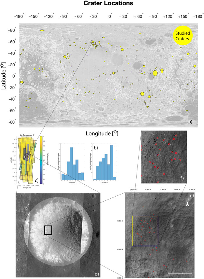
FIGURE 1. (A) Location of craters used for analysis [shown on a WAC shaded relief, 64 pixel/degree global mosaic (equidistant cylindrical projection) base map]. The size of the craters is scaled so that small craters also become visible in the figure. Exact details of crater location and size are given in Supplementary Material. (B) Longitude and latitude distributions of crater centers used in this study. (C) NAC image coverage of crater La Condamine B, the color indicates the resolution of each individual image. (D) One mosaic of crater La Condamine B (orthographic projection) built up from selected images displayed in (C). A magnified section, marked as a black rectangle in (D) is shown enlarged in (E) and expanded again in (F) to make some boulders and their tracks visible.
4.2 Method for boulder identification with tracks by a human analyst
The LRO mission (Robinson et al., 2010) has created a unique archive of lunar surface images that allows one to view a chosen lunar region from different orbital heights and from very different viewing directions and conditions, thereby generating images with different resolutions and phase angles. To systematically identify all the boulders with tracks in a particular crater in a repeatable workflow, the whole crater area has to be fully visible under viewing conditions which minimize the number of shadowed areas inside the crater rim and display the crater with the highest available resolution images. This condition is required for an AI and HA-based approach. If one clears the available data set of images that contain artifacts, as well as unfavorable signal-to-noise conditions, and only uses images that have sufficient resolution and favorable phase angle conditions, one would still face the problem of how to choose a minimum set of images to produce a mosaic for a selected crater using the given limited and possibly not optimal available images. As there are numerous possibilities to assemble such images into a mosaic, we have tried to automate the task of automatically finding the image arrangement that produces a mosaic that optimizes maximum crater surface visibility and spatial resolution, but in the end decided to choose the images for each crater after a visual inspection of the preselected images. The construction of a crater mosaic for the HA-based research in this study is described in more detail in Supplementary Figure S1.
We emphasize that the final image mosaic of a given crater in our case, which is analyzed by an HA, is not a single mosaicked image but a multi-layer mosaic cube. All the images that cover a particular crater are stacked on top of each other, thus producing an image cube. The stacking is thereby ordered based on a given criterion (spatial resolution, phase angle, etc.). The generated multi-layer mosaic of a particular crater allows one to investigate a given crater area on different NAC images, thereby creating the possibility to visually look at a particular crater location on multiple images that were taken at different resolutions and illumination conditions.
As the CNN-based search used pre-calibrated and compressed NAC pyramid image files without processing them through the standard USGS Integrated Software for Imagers and Spectrometers (ISIS) tool, the NAC pyramid image files used in this study were also not processed with this tool. This was done to avoid another potential new source of bias which could arise through the fact that the images we used would have been re-projected and corrected for various instrumental effects. For this reason, we also used the same cylindrical projection which was used in the original CNN workflow. By following the same procedure, we are confronted with the original issue in Bickel et al. (2020) that the position of individual boulders seen on different images has slightly different coordinate values. As we have in the HA-based approach the possibility to follow a track over the border of an image to the next adjacent image, we do not face the problem of mistakenly double counting the same boulder due to a shift in its location. We also note that we have used the same image pool that was available when the first study (Bickel et al., 2020) was conducted and did not add any newer images that became available since the CNN study was made.
By the time we finished our analysis, the LRO QuickMap image website had undergone several upgrades and improvements and now offered us the possibility to crosscheck our identified boulder positions on the fully ISIS-corrected images. We used these newly added possibilities to have an independent verification. All the boulder track searches were done by a trained geologist. In this way, all 181 craters were investigated and a grand total of 13,686 boulders were visually found and marked. In Figures 1D–F, one can see a close-up view of a tiny area (marked as a black rectangle in Figure 1D) of crater La Condamine B to show the corresponding boulders visible on the NAC image M1167354138R. Looking at the crossing of the numerous tracks (Figure 1F), it becomes clear how difficult it is even for an HA to identify the desired boulders.
For each of the 181 investigated craters, the location of each boulder was recorded, allowing one to generate a map of all the human-identified boulders and thereby allowing for a comparison with the boulder locations found through the CNN. The AI-identified boulders in a particular crater were found by reading the boulder coordinates of all boulders in the abovementioned boulder database and counting the entries that were found to be inside the area of the crater under investigation. The crater area and dimension were again taken from the LRO crater list (available from https://wms.lroc.asu.edu/lroc/rdr_product_select). For all investigated craters, the number of HA- and CNN-identified boulders with tracks was then tabulated (Supplementary Table S1).
Figure 2 is meant to exemplify one result of the comparison between the CNN-identified (red markers) and human-identified (black markers) boulders with tracks for the crater La Condamine B.
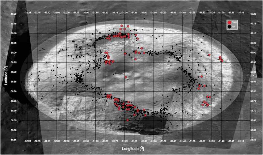
FIGURE 2. Comparison of identified boulders with tracks in crater La Condamine B. The background image shows a mosaic assembled from the study available NAC images in cylindrical equal-area projection. The mosaic is assembled from individual non–ISIS-corrected NAC images which have a different spatial resolution (below 1 m/pixel).
4.3 Investigation of accuracy of identification
The standard metrics (accuracy, ROC, etc.) from the CNN study were computed based on the whole data set. As we could not repeat the HA-based search with several individuals, we did not have the intention to produce an absolute comparison of the absolute sensitivities of the two approaches in identifying boulders with tracks. Our main goal for this investigation was to estimate how an HA-based approach compares with a CNN-driven workflow and understand what could explain the possible differences in the number of identified boulders, with the intention to identify major shortcomings in the CNN-driven approach to boost the sensitivity of future AI-driven workflows. By analyzing the 181 craters which differ in size and were chosen from all over the lunar surface, we could see systematic differences in the results that the two approaches deliver.
Once a mosaic with minimum shading and the best available spatial resolution for a given crater has been produced, the task given to a trained HA of finding all the boulders with tracks in a given crater is in principle straightforward. It is essentially a question of time and the steady concentration of the analyst. The human verification of a boulder with a track identified by the CNN is, however, a much more difficult task to achieve. There are several reasons responsible for this fact. The localization of a given boulder in a given LRO NAC image is often difficult to find due to the following factors: the size of the NAC images relative to the size of the boulders in it (Figure 1), resolution of the image, particular illumination conditions of the scene at the time the image was taken, and possible shift in coordinates of the boulder coordinates (taken from the AI boulder database) from the position where the boulder is seen in the image. The observed deviation of the true boulder position from the computed boulder position is caused by the fact that the expected selenographic boulder coordinates in the image have to be computed directly from the four selenographic corner coordinates of the image, and no full projection of the image onto a digital elevation model (DEM) is made. This shortcut in the original AI workflow was made because a full mapping of the NAC image onto the lunar DEM using the ISIS to obtain the exact (geographically and optically corrected) selenographic image coordinate of the individual pixels would have been extremely CPU-time intensive. Complications of verifying a particular boulder listed in the database on an image can also be caused by nearby tracks and boulders with tracks that were not found by the CNN and the abovementioned coordinate shift of the listed boulder coordinates.
To verify in each of the 57,876 images the boulder locations that the CNN found, a workflow had to be designed that allowed a fast process for finding and looking at these locations in each individual image. This was achieved through the following process (Figure 3).
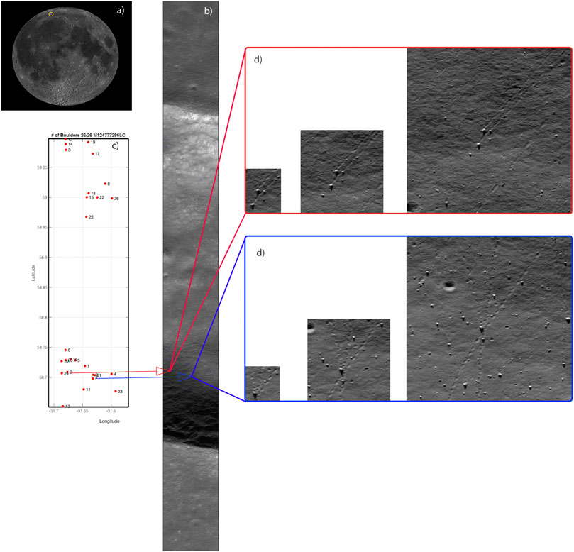
FIGURE 3. (A) Lunar location of crater La Condamine B. (B) Unprojected LROC NAC file M124777286LC with highlighted CNN localized boulders. (C) Locations of boulders identified in AI workflow projected onto a cylindrical equal-area projection map. (D) Zoomed image regions (small, medium, and large) of NAC image shown in (B) of two boulder locations specified in the boulder database.
Figure 3 gives an overview of the individual steps involved in this process (again for crater La Condamine B). The location of the crater is marked in Figure 3A. In order to check how many boulders with tracks the CNN workflow has found inside this crater, every boulder entry in the database with coordinates inside this crater has to be looked up by the HA. For every NAC image, which is associated with a boulder inside the crater under investigation (Figure 3B), a map covering the crater boundary in the image was produced in which the computed boulder locations were marked and numbered (Figure 3C). On the NAC image itself, three boxes (Figure 3D) of variable sizes (small, medium, and large) around every CNN-identified boulder location were selected, so that the expected boulder location could be visualized and compared with the map. The pixel content in the three boxes containing the CNN-identified boulder was then stored as three individual images. These images were then labeled with the identifier that the boulder was originally given in the CNN boulder catalog. Using the boulder map together with the NAC image containing the marked image position allows for a repeatable workflow for inspecting each CNN-identified boulder. By looking at the image sequence from small, medium, and large (Figure 3D), an analyst can come to a clear decision whether the CNN found a true boulder or whether the recorded boulder could be a candidate for a misclassification which occurred.
Looking at Figure 3D shows that it is straightforward for an HA to decide whether he is looking at an image that contains a boulder with a track or not. In all the cases where he is not sure what he sees, he can look at the multi-layer crater mosaic that was produced for the crater (or he can now also consult the new upgraded LROC QuickMap website) to inspect the corresponding location where the boulder is supposed to exist. Looking at the same position on the different images that make up the multi-layer crater mosaic where a problematic boulder identification has occurred allows the HA in most cases to resolve the issue of whether this has been a true positive identification or whether the algorithm has produced a false positive event.
5 Results
The results of our boulder search and verification process are summarized in Supplementary Table S1. Displayed for each crater are the name, location of the crater center in degrees (latitude, longitude), radius in kilometers, number of boulders identified with the help of the CNN [boulder (CNN)], the number of boulders found by the CNN (Bickel et al., 2020b) and verified by a human [boulder (CNN verified)], the number of boulders found by an HA [boulder (HA)], and ratio of boulders found by the CNN to the number of boulders found by the HA (CNN/HA). Figure 4 summarizes the main results and shows the location of each investigated crater together with the relative number of boulders found by the CNN and HA as a pie chart (yellow denotes the fraction identified by the HA and red is the fraction as seen by the CNN approach). Craters marked as black areas are craters where no boulders with tracks were identified by both approaches. Craters marked as red are craters where only the CNN approach identified rolling boulders but none were found by the HA. We discuss this particular case in detail below. In total, we have identified 13,686 boulders with tracks in the HA search when compared to 1,806 boulders (we counted all boulders found by the CNN not distinguishing between true positives or false positives) found by the CNN. With approximately 15%, it becomes clear that the HA approach beats the CNN-driven workflow hands down. By inspecting inserts Figure 1E and Figure 1F in Figure 1, one notices that a given track pattern in an image can be very complex due to multiple crossings of tracks. Given the fact that the images have their intrinsic limited resolution, an HA-based and AI-based analysis could both have a problem associating individual tracks to the rolling boulders that had produced them. This may lead to a situation where two different HAs locate boulders at different positions. The exact reproducibility of results found by an applied AI algorithm is an advantage here as compared to an HA. We also have to point out that we found numerous cases where the boulder positions given in pixel coordinates in the boulder database did not fit inside the selenographic boundary of the associated image coordinates. We assume that such listings originated during the compilation of data for the archive. Furthermore, we note that the number of boulders in craters that have a radius smaller than 5 km can be rather small. The important point we make is that there are systematic effects at work that lead to the difference in the observed results delivered by the HA and AI and resulted in the underperformance of the AI workflow. We are detailing our reasoning for this underperformance in the following paragraph.
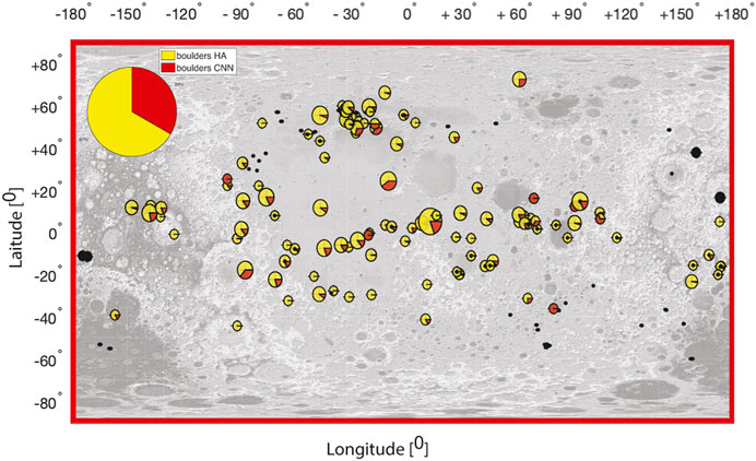
FIGURE 4. Same map as shown in Figure 1A but now crater locations are replaced with a pie chart showing the fraction of boulders found by an HA (yellow) compared to boulders found by the CNN (red) at each investigated crater location (the detailed values for each crater are given in Supplementary Table S1).
6 Understanding the underperformance of the CNN approach
Our analysis makes it clear that the CNN’s performance in the earlier study cannot compete with human-based analysis. It is now of crucial importance to gain an understanding of where potential differences in the ability to recognize boulders with tracks between the AI-identified results and human-based investigation could originate from. To investigate this question, we looked at two aspects: first, has the CNN workflow really received the required information from the images to identify boulders, and second, given that this information was indeed available to the AI workflow, what led to a misidentification of a particular boulder? Sufficient image resolution, good signal-to-noise ratio, phase angle selection, and image exposure time are obviously not sufficient criteria to guarantee that AI is in a position to find all the boulders with tracks in an image. The areas in a given crater are often shaded to a certain extent, and therefore no information can be extracted from these regions (we exemplify this point in the supplement with Supplementary Figure S2). To find out whether such a partial shading effect is randomly distributed or not, we grouped all boulder entries in the database according to the image ID on which these were found. Each identified boulder was then associated with the available metadata of the image on which the boulder was detected, thereby allowing one to check under which observational conditions the boulders were identified by the CNN. By visualizing the image boundaries of the 57,876 NAC images on a map, areas where no boulders were identified by the CNN show up as white space. Figure 5 shows the coverage of the lunar surface by the NAC frame boundaries compiled in the boulder database.
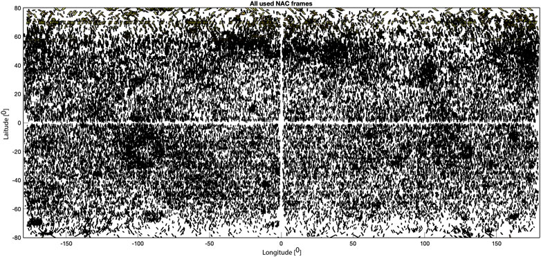
FIGURE 5. Distribution of NAC frames which contains at least one CNN-identified boulder.
Visible in this figure are two kinds of white spaces: the white cross separating the four map quadrants resulted obviously from the way the individual images were fed into the CNN. This feature is an artifact resulting from an imperfect workflow. The other areas on the map that are white denote places where the CNN did not find any boulders. One has to keep in mind that a white region on the map does not necessarily indicate that this particular lunar area was not covered by an image or no boulder identification took place. The reason for this is as follows. An identified boulder was stored only once in the database even when the CNN may have recognized it on more than one image (each with their different associated image boundaries). Regions may show up on the map as white areas because the boulder associated with this particular area was already found on another image. In the case where the image boundaries that contain the boulder are overlapping, only one image name was stored in the database. Despite the fact that we cannot retrieve the missing image name from the database, we will show below how we can still make a statement on whether the CNN was missing image information in a given region of a crater area.
To understand whether the boulder-free areas are intrinsically free of boulders or whether the areas are free of boulders because of observational and/or AI-related issues, we investigated all 181 craters in terms of resolution and phase angle. Figure 6 displays the crater area of La Condamine B with the boundaries of the images that are found in the database catalog and cover this particular crater area. The number of times a surface area is covered by an image is color-coded. This type of target area image coverage analysis allows one to recognize whether a particular crater area is covered multiple times in the image selection process or not.
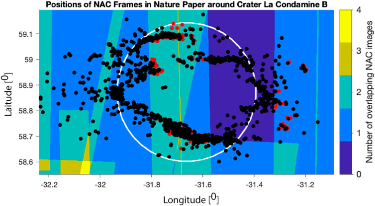
FIGURE 6. Image coverage analysis of crater La Condamine B.
Superimposed on this image are the locations where rolling boulders were identified by the HA (black points) and CNN workflow (red points). One can clearly notice that there are areas that were not covered by an image and that in these areas, the HA could identify plenty of boulders.
As this was a repeating pattern that we could observe in all investigated craters, one can assume that the CNN either did not process the adjacent images or certain parts of these images did not contain sufficient information, potentially due to insufficient image resolution or unsatisfactory surface illumination which may have caused a substantial shadowing. To investigate the issue of a possible shading of parts of the crater area, a measure for the shadowing effect must be defined. We have found that in the 8-bit NAC images, pixel values smaller than 20 are too dark for the human annotator to extract information on the location of the boulders. We have therefore computed the fraction of all pixel values smaller than 20 to the sum of all pixels in an individual image frame, so that a completely dark image frame would have a value of 1. In Figure 7, we display the center location (latitude/longitude coordinate) of all the individual NAC images stored in our boulder catalog which have a shading factor greater than 25% as circles. The radius of the circles scales with the fraction of the image which is too dark to be used for the detection of the boulders. The non-homogenous distribution of the frames that have dark areas as shown in the figure clearly demonstrates that a shading analysis must be implemented for the selection of images that are fed into the CNN. A phase angle selection criterion alone is not sufficient to guarantee a non-biased global boulder map.
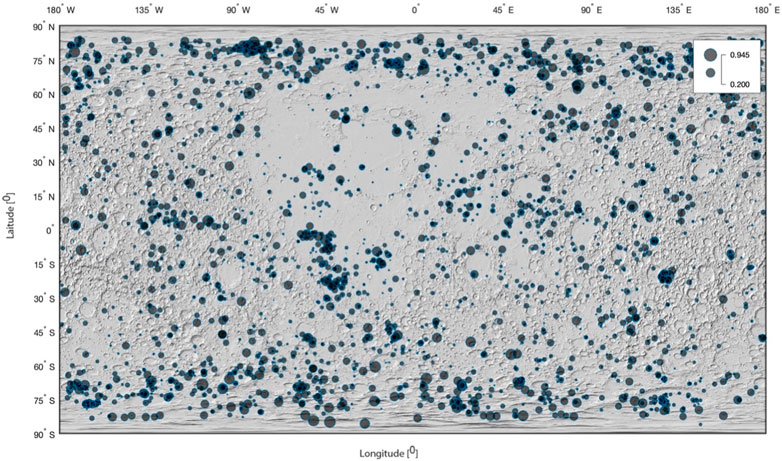
FIGURE 7. Location of NAC frames in the boulder database which shows substantial shading. Shown for each image frame is the unitless ratio of pixel values smaller than 20 to the sum of all pixel values in a frame. The ratio is displayed at the selenographic coordinate center of each frame.
We now turn to the question of what causes the misidentification of boulders. Once we identified the boulders that were misidentified using the above-described method (Section 4.3), we were interested in understanding the cause of the misclassifications that we found. Therefore, various groupings were formed with the goal of collecting similar surface features in the images around a misidentified boulder which could be responsible for a false classification by the CNN. Based on our inspection, we could form six categories of misclassified boulders. The groups are named as follows:
• “Shadows as a track”
• “Morphological structures as track”
• “Rock next to or on a track”
• “Smaller craters as track”
• “Beginning of the track”
• “Unknown error source”
As the names imply, each group has its own characteristics. However, the boulder area around a misclassified boulder can show the characteristic features of more than one group. In this case, it is not obvious which of the features was responsible for the classification.
In the following, we present from each group, a representative image to illustrate the image categories which the CNN repeatedly misclassified. The most general source for a misclassification which can occur in all categories is the situation where a crater is being interpreted as a boulder. All figures contain projected NAC images and selected zoomed areas of interest. On the LRO QuickMap website, these areas can be displayed in equidistant, orthographic projection or on the lunar globe.
The group “shadow as a track” consists of cases when a boulder track is mimicked by the end of the shadow which a crater or rock casts. The example is taken from the NAC image M1254331878R shown in Figure 8A. Figure 8B shows such an example of a false positively classified CNN boulder with a track event. In the image frame (shown in Figure 8B), it is not clear whether we are dealing with a crater and rille-like structure adjacent to a small crater or a boulder with an excavated track part. Knowledge of the illumination direction of the scene would allow one to distinguish between these two cases as the surface topography would dictate the observed sequence of shadows cast in the scene. Larger sections of the image at the identified boulder location (Figure 8C) with multiple small craters instantly give it away from the direction that the Sun illuminates the surface (marked with arrows in Figure 8C). Based on the direction of the Sun’s light, an illuminated boulder or rock should therefore show first a brighter and then a darker area. The light and dark areas of a boulder should be in the reverse order when compared to the track. As shown in Figure 8B, the round object and misidentified track follow the same scheme, so that a boulder/rock and track can be excluded. We note that in this category, the shadows can have various origins.
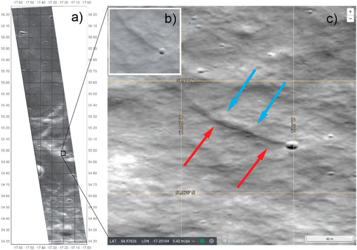
FIGURE 8. Example of a false positive event from the CNN classification from the “shadows as a track” group. (A) Projected NAC image M1254331878R. (C) Enlarged area marked in (A) with a box. (B) CNN image of an identified boulder with tracks.
In the category “morphological structures as tracks,” geomorphological structures are recognized as tracks. In this group, a boulder or crater sits at the end of a misidentified track.
Figure 8A shows the NAC image M1254803528L from which this example is taken. The CNN image of the classified boulder is shown in Figure 9D. Two dark lines can be seen which run parallel to each other (marked by blue arrows in the image).
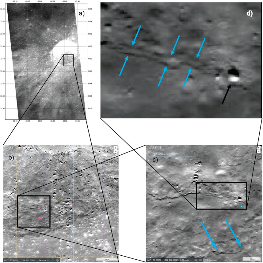
FIGURE 9. Example of misidentification from the group “morphological structures as traces.” (D) shows a boulder with a cliff at its end, causing two dark lines with constant distance. (B, C) show larger sections of the image (A). The edge of the crater is visible at the lower end (C). The misidentified track is perpendicular to the fall direction/center of the crater.
At the end of the lines, a rock is clearly visible (black arrow). It is difficult for the observer to recognize whether the lines are a track or not. By looking at a larger section of the image Figure 9C, one can recognize that the two lines are part of a crater wall. The example should make it clear how important the choice of an appropriate map projection can be. Using non-conformal map projections can lead to non-circular shapes of craters and unnatural shapes of boulders. Depending on the latitude of the object under consideration, either the AI or HA can be deceived by interpreting strongly distorted crater walls as rille-like structures or boulders as craters. In the lower part of the image, the edge of the crater can be seen (marked by green arrows). The cliff, which has been identified as a track, is perpendicular to the fall direction/center of the crater. Therefore, the two dark parallel running lines can be ruled out as a boulder track. Other morphological structures that lead to misidentification in this category are landslides or cracks on the crater wall.
The next category “rock next to or on a track” pools events in which a rock is next to or on a real track. In a few cases, there is also a crater next to the track, which has been falsely identified as a boulder. In Figure 10B, one can see a track produced by a bouncing boulder. Inside and outside the track, several boulders are visible. As we have no information on the rocks that have been identified as boulders by the CNN, the image represents both cases (rock is next to or on a real track) of misidentifications that occur in this category. In both cases, the boulder track is real and has been correctly identified, but the associated boulder is probably incorrectly assigned. The two larger boulders in Figure 10B (blue arrows) are next to the track and can therefore be excluded as the associated boulder. The rock inside the track (red arrow) is too small to create a large track. In addition, the track continues to the left and right of the rock. For this reason, the rock can be excluded as an associated boulder. There are three plausible explanations for why the rock lies on the track. First, an older boulder was rolled over by the larger boulder, thereby erasing the track of the smaller boulder. Second, it is a fragment of the larger boulder that rolled down the hillside, or third, the boulder rolled into the bigger track that was already there. Other possibilities can, of course, also not be ruled out, as the track could have already been made unrecognizable by erosion. Due to the smaller size of the track, this would take less time than it does for the large track. However, all three presented explanations have in common that the large track does not match the smaller rock and therefore the rock was definitively incorrectly identified by the neural network.
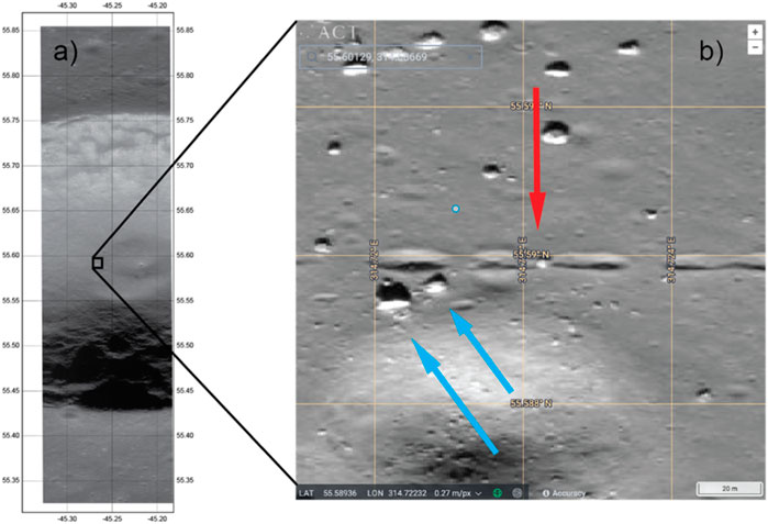
FIGURE 10. Example of misidentification from the category “boulders next to or on a track.” (A) NAC image M140201925L. (B) Rocks that are inside and outside a track. None of the rocks belong to the track.
In the category “smaller craters as track,” rocks or larger craters are surrounded by smaller craters that more or less form a straight line. In Figures 11A, B, a larger crater is seen (red arrow), which has been identified as a boulder. Southeast of the larger crater, several smaller craters are visible (blue arrows), which form a straight line. The smaller craters were incorrectly identified as a track. Presumably, the smaller craters were interpreted as a track from a bouncing boulder. In the larger image section, it becomes more obvious that the misidentified track consists of smaller craters. There is no sign of a track or boulder in the image.
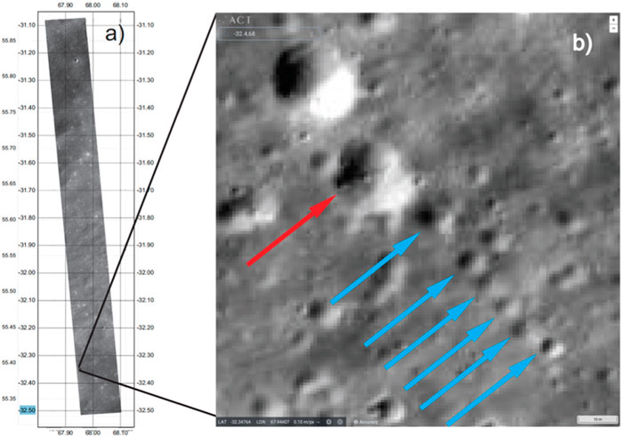
FIGURE 11. Example of misidentification from the “smaller craters than trace” category. (A) NAC M1251463987L. (B) Several smaller craters forming a straight line. At its end is a larger crater. The smaller craters were misidentified as a track and the larger crater as a boulder. On a larger section of the image, there is no sign of a track or boulder.
“Beginning of track” is a category where the beginning of a track has been identified as its end. As can be seen in Figure 12B (insert with blue arrow), there is a darker area (blue arrow) at the end of the track. This area was incorrectly identified as a boulder. In a larger image section, one can notice that this is the beginning and not the end of the track. The potentially associated boulders of the track are marked with red arrows. In many cases in this category, the boulder, and thus the beginning of the track, comes from a cliff or a cluster of rocks. Both ends of the track could be recognized as boulders by the AI, which does not seem to recognize whether the track or boulder rolled in the direction of the slope and thus into the center of the crater.
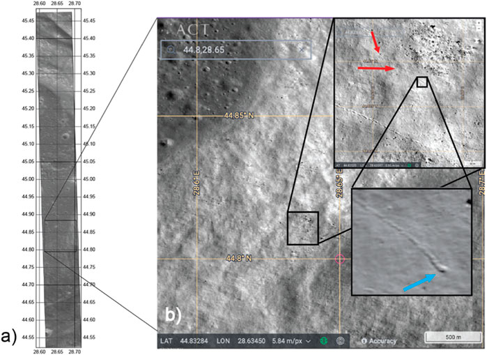
FIGURE 12. Example of a false identification from the “beginning of a track” group. (A) NAC image M170368202R. (B) Enlargement of the image area marked with a black box that is shown in (A) and several inserts that subsequently enlarge the corresponding black boxes displayed in the image. The CNN-identified structure (marked with a blue arrow in the highest magnified image) was incorrectly identified as a boulder by the artificial intelligence. At an extended image section, one can see the corresponding boulder of the track (red arrows).
The “unknown error source” category contains by far the highest number of events that were falsely classified by the CNN. It is difficult for the observer to classify these images into the previously mentioned categories. In most cases, it is not obvious which object the artificial intelligence has identified as a boulder and which as a track. For example, Figure 13A shows a rock cluster consisting of many small boulders (recognizable as white dots). Which rock the artificial intelligence has identified as a boulder is not comprehensible. A track is also not visible. In Figure 13B, many smaller tracks can be misinterpreted due to the morphological structure and shadows. However, a crater or rock is missing as a possible recognized boulder. In Figure 13C, there are many craters that could be recognized as a boulder. However, neither prominent morphological structures nor smaller craters that could be recognized as a track are visible.
FIGURE 13. Examples of misidentification from the “unknown error source” category. In all figures (A–C), it is not obvious what the AI has identified as a boulder or track. For this reason, an accurate classification into a category is not possible.
7 Summary and discussion
As the use of information from AI-driven approaches in geomorphology is quickly spreading and the quality of this information becomes more difficult to check, the main performance indicators for a CNN, the accuracy of AI-driven approaches, have to be carefully assessed before their usage. The achieved accuracy not only relies on the architecture of the network itself but also on factors like the data chosen for training, the training process, and the verification process. Networks themselves can be scaled up in different ways to achieve better accuracies. The accuracy of a CNN is usually evaluated by using an operational data set (unlabeled real-world data), from which a subset is selected, manually labeled, and used as the test set. This subset should faithfully represent the operational context, with the resulting test suite containing roughly the same proportion of examples causing misclassifications as the operational data set. If beyond the distribution of training samples (InD data), OOD data exist, which may not belong to any of the classes that the model is trained on, one can expect a significant impact on the classification accuracy. An essential question is therefore whether in the training phase, the selection of the training samples leads to a bias which ultimately makes the statistical data practically unsuitable for answering the specific question under investigation. Moreover, in geomorphological studies that use remote sensing data to find the features of OOD, it may already be impossible as the resolution is very often too low to clearly define such data groups.
In this work, we compared the quality of the results produced by an AI and HA approach to identify specific surface features in a geomorphological study using the same high-resolution data set (LROC NAC images). The CNN identified 136,610 lunar boulders associated with tracks in an archive of more than 2 million high-resolution images to produce the first global map of 136,610 lunar rockfall events.
To accomplish the goal of comparing the quality of the identification capability of identifying boulders with tracks on the lunar surface by the given AI approach and HA approach, 181 lunar craters of variable sizes from the same latitude/longitude range as the AI-driven study covered have been selected. For the HA-identification approach, crater mosaics using the same image pool, which was fed into the AI-driven data pipeline, were used. In this process, multi-layer NAC image mosaics were produced using the same location information that was available to the AI workflow. The search for boulders with tracks was done on these multi-layer NAC image mosaics and on the LRO NAC QUICKMAP website. The number of boulders identified with tracks found by the HA was compared with the number of craters identified by the AI-driven approach for all 181 craters and then tabulated. In an attempt to understand the misidentifications of the AI-driven approach, the locations of the AI-identified boulders on the recorded images were identified and visualized. By visual inspection of the misidentified boulders, groups were formed which shared common features to identify what caused the misidentifications. The investigation revealed an extreme discrepancy between the number of boulders identified with the help of the CNN and that found by the HA which can surpass a factor of 100.
In an attempt to understand the underperformance of the CNN, individual misclassifications by the CNN were identified and grouped with the goal of collecting similar surface features in the images around a misidentified boulder. The analysis showed that the misidentifications in the groups were mainly caused by the fact that the CNN classified shadows, morphological structures, rocks, or smaller craters as tracks.
8 Conclusion
CNNs are able to identify boulders with tracks. Neural networks, which have become widely available through various program libraries, are well suited to investigate the distribution of these boulders on planetary surfaces. However, for quantitative statistically relevant results, out-of-the box CNNs which use a brute force approach to feed images into an identification workflow are not able to come close to the quality which a human analyst-based approach can deliver. The fact that we found numerous examples where the CNN identified no boulders with tracks in craters whereas the human analyst found hundreds of them demonstrates this point clearly. We also clearly show that a selection of input images based on image resolution, phase angle, and image exposure time is not sufficient to ensure that surfaces to be scanned for a specific feature are statistically sufficiently sampled to produce a balanced input data set. Topographic and illumination scene information should be implemented in future AI mapping efforts of the kind that we investigated. Our studies have also shown that a referencing of boulders based on the four corners’ latitude/longitude coordinates of an NAC image may lead to multiple counting of the same boulders on different NAC images. To gain relevant statistical information about a boulder population, individual geometric pixel coordinates must be precisely known, which can only be ensured by using the ISIS data pipeline. The resulting data sets have to be scrutinized at least partially with conventional imaging methods to ensure proper verification of the AI-based results. Our results also indicate that training sets should be generated in a reproducible process and require a sampling and data analysis plan with full documentation. In particular, we recommend that researchers in geophysical disciplines collaborate closely with their colleagues in the AI field who develop these tools. In view of the findings of this research, we reconsider the question of whether lunar mass wasting is primarily driven by impact and whether impact-induced fracture networks are to be again an open question.
Data availability statement
Only publicly available data sets were used and analyzed in this study. The boulder data sets used in this research were made publicly available (accessible https://doi.org/10.17617/3.OG927P). Lunar images can directly be viewed at https://quickmap.lroc.asu.edu/ and downloaded from https://wms.lroc.asu.edu/lroc/ search and the auxiliary data can be downloaded from https://www.usgs.gov/products/web-tools/data-access-tools and https://wms.lroc.asu.edu/lroc/rdr_product_select.
Author contributions
UM designed the conceptualization of the work, constructed the multi-layer crater images, and wrote the draft of the manuscript. DK identified all the boulders on the LROC QuickMap images, reviewed the labeling of the boulder data archive, produced the false classification grouping of the CNN, and wrote the section which describes this classification. UM compared the boulder identification on the multi-layer images with the results from the QuickMap identification. PL contributed to the various stages in designing the boulder identification software, mapping of the lunar images, and AI simulations. DK and PL provided comments and edits for the improvement of the manuscript. UM, DK, and PL agreed to be accountable for the content of the work. All authors contributed to the article and approved the submitted version.
Funding
The funding for this work was provided through the Max-Planck Society.
Acknowledgments
We thank the LROC team for LRO NAC data used here and the development and refinement of the LROC QuickMap website.
Conflict of interest
Author PL was employed by MathWorks and is now at Databricks.
The remaining authors declare that the research was conducted in the absence of any commercial or financial relationships that could be construed as a potential conflict of interest.
Publisher’s note
All claims expressed in this article are solely those of the authors and do not necessarily represent those of their affiliated organizations, or those of the publisher, editors, and reviewers. Any product that may be evaluated in this article, or claim that may be made by its manufacturer, is not guaranteed or endorsed by the publisher.
Supplementary material
The Supplementary Material for this article can be found online at: https://www.frontiersin.org/articles/10.3389/fspas.2023.1176325/full#supplementary-material
References
Basilevsky, A. T., Head, J. W., and Horz, F. (2013). Survival times of meter-sized boulders on the surface of the Moon. Planet. Space Sci. 89, 118–126. doi:10.1016/j.pss.2013.07.011
Bickel, V., Lanaras, C., Manconi, A., Loew, S., and Mall, U. (2019). Automated detection of lunar rockfalls using a convolutional neural network. IEEE Trans. Geoscience Remote Sens. 57, 3501–3511. doi:10.1109/TGRS.2018.2885280
Bickel, V. T., Aaron, J., Manconi, A., Loew, S., and Mall, U. (2020). Impacts drive lunar rockfalls over billions of years. Nat. Commun. 11, 2862. doi:10.1038/s41467-020-16653-3
Bickel, V. T., Conway, S. J., Tesson, P.-A., Manconi, A., Loew, S., and Mall, U. (2020b). Deep-learning-Driven detection and mapping of rockfalls on mars. IEEE J. Sel. Top. Appl. Earth Observations Remote Sens. 13, 2831–2841. doi:10.1109/JSTARS.2020.2991588
Boulton, G. S. (1978). Boulder shapes and grain-size distributions of debris as indicators of transport paths through a glacier and till genesis. Sedimentology 25, 773–799. doi:10.1111/j.1365-3091.1978.tb00329.x
Bourrier, F., Berger, F., Tardif, P., Dorren, L., and Hungr, O. (2012). Rockfall rebound: comparison of detailed field experiments and alternative modelling approaches. Earth Surf. Process. Landforms 37 (6), 656–665. doi:10.1002/esp.3202
Dagar, A. K., Rajasekhar, R. P., and Nagori, R. (2022). Analysis of boulders population around a young crater using very high resolution image of Orbiter High Resolution Camera (OHRC) on board Chandrayaan-2 mission. Icarus 386, 115168. doi:10.1016/j.icarus.2022.115168
DeLatte, D. M., Crites, S. T., Guttenberg, N., and Yairi, T. (2019). Automated Crater detection algorithms from a machine-learning perspective in the convolutional neural network era. Adv. Space Res. 64 (8), 1615–1628. doi:10.1016/j.asr.2019.07.017
Deng, L., and Yu, D. (2014). Deep-learning methods and applications. Found. Trends Signal Process. 7 (Nos 3-4), 197–387. doi:10.1561/2000000039
Dunlop, H., Thompson, D. R., and Wettergreen, D. (2007). Multi-scale features for detection and segmentation of rocks in mars images. IEEE Conf. Comput. Vis. Pattern Recognit., 1–7. doi:10.1109/CVPR.2007.383257
Fanara, L., Gwinner, K., Hauber, E., and Oberst, J. (2020). Automated detection of block falls in the north polar region of Mars. Planet. Space Sci. 180, 104733. doi:10.1016/j.pss.2019.104733
Feldens, P. (2020). Super resolution by deep learning improves boulder detection in side scan sonar backscatter mosaics. Remote Sens. 12, 2284. doi:10.3390/rs12142284
Feldens, P., Westfeld, P., Valerius, J., Feldens, A., and Papenmeier, S. (2021). Automatic detection of boulders by neural networks. HENRY Hydraul. Eng. Repos. doi:10.23784/HN119-01
Fukushima, K. (1980). Neocognitron: a self-organizing neural network model for a mechanism of pattern recognition unaffected by shift in position. Biol. Cybern. 36, 193–202. doi:10.1007/bf00344251
Glassmeier, K. (2020). Solar system exploration via comparative planetology. Nat. Commun. 11, 4288. doi:10.1038/s41467-020-18126-z
Golombek, M., Huertas, A., Kipp, D., and Calef, F. (2012). Detection and characterization of rocks and rock size-frequency distributions at the final four mars science laboratory landing sites. Int. J. Mars Sci. Explor. 7. doi:10.1555/mars.2012.0001
Golombek, M. P., Trussell, A., Williams, N., Charalambous, C., Abarca, H., Warner, N. H., et al. (2021). Rock size-frequency distributions at the InSight landing site, Mars. Earth Space Sci. 8, e2021EA001959. doi:10.1029/2021EA001959
Hinton, G. E., and Salakhutdinov, R. R. (2006). Reducing the dimensionality of data with neural networks. Science 313, 504–507. doi:10.1126/science.1127647
Khajavi, N., Quigley, M., McColl, S. T., and Rezanejad, A. (2012). Seismically induced boulder displacement in the port hills, New Zealand during the 2010 darfield (canterbury) earthquake. N. Z. J. Geol. Geophys. 55 (3), 271–278. doi:10.1080/00288306.2012.698627
McGovern, A., and Wagstaff, K. L. (2011). Machine-learning in space: extending our reach. Mach. Learn 84, 335–340. doi:10.1007/s10994-011-5249-4
Molaro, J. L., Byrne, S., and Langer, S. A. (2015). Grain-scale thermoelastic stresses and spatiotemporal temperature gradients on airless bodies, implications for rock breakdown. J. Geophys. Res. Planets 120, 255–277. doi:10.1002/2014je004729
Pajola, M., Pozzobon, R., Lucchetti, A., Rossato, S., Baratti, E., Galluzzi, V., et al. (2019). Abundance and size-frequency distribution of boulders in Linné crater's ejecta (Moon). Planet Space Sci. 165, 99–109. doi:10.1016/j.pss.2018.11.008
Pajola, M., Rossato, S., Baratti, E., Pozzobon, R., Quantin, C., Carter, J., et al. (2017). Boulder abundances and size-frequency distributions on Oxia Planum-Mars: scientific implications for the 2020 ESA ExoMars rover. Icarus 296, 73–90. doi:10.1016/j.icarus.2017.05.011
Palafox, L. F., Hamilton, C. W., Scheidt, S. P., and Alvarez, A. M. (2017). Automated detection of geological landforms on mars using convolutional neural networks. Comput. Geosciences 101, 48–56. doi:10.1016/j.cageo.2016.12.015
Regmi, N. R., Giardino, J. R., McDonald, E. V., and Vitek, J. D. (2015). A review of mass movement processes and risk in the critical zone of Earth. Dev. Earth Surf. Process., 319–362. doi:10.1016/b978-0-444-63369-9.00011-2
Robinson, M. S., Brylow, S. M., Tschimmel, M., Humm, D., Lawrence, S. J., Thomas, P. C., et al. (2010). Lunar reconnaissance orbiter camera (LROC) instrument overview. Space Sci. Rev. 150, 81–124. doi:10.1007/s11214-010-9634-2
Ruj, T., Komatsu, G., Kawai, K., Okuda, H., Xiao, Z., and Dhingra, D. (2022). Recent boulder falls within the Finsen crater on the lunar far side: an assessment of the possible triggering rationale. Icarus 377, 114904. doi:10.1016/j.icarus.2022.114904
Schroder, S., Carsenty, U., Hauber, E., Raymond, C., and Russell, C. (2021a). The brittle boulders of dwarf planet Ceres. Planet. Sci. J. 2, 111. doi:10.3847/psj/abfe66
Schroder, S. E., Carsenty, U., Hauber, E., Schulzeck, F., Raymond, C. A., and Russell, C. T. (2021b). The boulder population of asteroid 4 Vesta: size-frequency distribution and survival time. Earth Space Sci. 8. doi:10.1029/2019EA000941
Senthil Kumar, P., Mohanty, R., Lakshmi, K. J. P., Raghukanth, S. T. G., Dabhu, A. C., Rajasekhar, R. P., et al. (2019). The seismically active lobate scarps and coseismic lunar boulder avalanches triggered by 3 january 1975 (MW 4.1) shallow moonquake. Geophys. Res. Lett. 46, 7972–7981. doi:10.1029/2019gl083580
Senthil Kumar, P., Sruthi, U., Krishna, N., Lakshmi, K. J. P., Menon, R., Amitabh Gopala Krishna, B., et al. (2016). Recent shallow moonquake and impact-triggered boulder falls on the moon: new insights from the Schrödinger basin. J. Geophys. Res. Planets 121, 147–179. doi:10.1002/2015JE004850
Ulrich, V., Williams, J. G., Zahs, V., Anders, K., Hecht, S., and Hoefle, B. (2021). Measurement of rock glacier surface change over different timescales using terrestrial laser scanning point clouds. Earth Surf. Dyn. 9, 19–28. doi:10.5194/esurf-9-19-2021
van der Bogert, C. H., Clark, J. D., Hiesinger, H., Banks, M. E., Watters, T. R., and Robinson, M. S. (2018). How old are lunar lobate scarps? 1. Seismic resetting of crater size-frequency distributions. Icarus 306, 225–242. doi:10.1016/j.icarus.2018.01.019
Vijayan, S., Harish Kimi, K. B., Tuhi, S., Vigneshwaran, K., Sinha, R. K., et al. (2022). Boulder fall ejecta: present day activity on Mars. Geophys. Res. Lett. 49, e2021GL096808. doi:10.1029/2021GL096808
von Rönn, G. A., Schwarzer, K., Reimers, H.-C., and Winter, C. (2019). Limitations of boulder detection in shallow water habitats using high-resolution sidescan sonar images. Geosciences 9 (9), 390. doi:10.3390/geosciences9090390
Keywords: geomorphology, deep learning, rock boulders, lunar craters, remote sensing
Citation: Mall U, Kloskowski D and Laserstein P (2023) Artificial intelligence in remote sensing geomorphology—a critical study. Front. Astron. Space Sci. 10:1176325. doi: 10.3389/fspas.2023.1176325
Received: 28 February 2023; Accepted: 31 October 2023;
Published: 30 November 2023.
Edited by:
Francesca Altieri, Institute for Space Astrophysics and Planetology (INAF), ItalyReviewed by:
Lucia Marinangeli, University of Studies G. d'Annunzio Chieti and Pescara, ItalyYuri Velikodsky, National Aviation University, Ukraine
Copyright © 2023 Mall, Kloskowski and Laserstein. This is an open-access article distributed under the terms of the Creative Commons Attribution License (CC BY). The use, distribution or reproduction in other forums is permitted, provided the original author(s) and the copyright owner(s) are credited and that the original publication in this journal is cited, in accordance with accepted academic practice. No use, distribution or reproduction is permitted which does not comply with these terms.
*Correspondence: Urs Mall, bWFsbEBtcHMubXBnLmRl