High-resolution permittivity estimation of ground penetrating radar data by migration with isolated hyperbolic diffractions and local focusing analyses

1 Introduction

Ground penetrating radar (GPR) is important for detecting shallow subsurface structures, which has been successfully used on the Earth, Moon, and Mars (Boisson et al., 2009; Jordan et al., 2009; Fang et al., 2014; Xiao et al., 2015; Zhang et al., 2015; Schroeder et al., 2019; Hamran et al., 2020; Zhou et al., 2020; Oudart et al., 2021; Zhang X et al., 2021; Li et al., 2022). However, it is difficult to analyze the underground velocity because the observation system of the GPR is almost zero-offset (i.e., the transmitter and the receiver are close to each other in position), which has no enough number of multiple offsets (Su et al., 2014; Zhang et al., 2014; Fa et al., 2015; Feng et al., 2019). Consequently, we can only estimate the velocity using methods originally developed for zero-offset data (Economou et al., 2020; Leong and Zhu, 2021). Fortunately, the zero-offset radar profiles are similar to the post-stack seismic profiles; thus, we can take the benefits of the velocity estimation methods that were developed in seismic exploration field for post-stack seismic profiles (Claerbout, 1985; Zhu et al., 1998; Hu et al., 2001; Fomel et al., 2007; Reshef and Landa, 2009; Carpentier et al., 2010).

The simplest method of velocity estimation is to assign a constant velocity for each identifiable layer, assuming that there is no lateral variation in each layer (Dai et al., 2014; Li et al., 2017). Undoubtedly, this method would encounter great uncertainty because it is difficult to evaluate the accuracy of velocity estimations. Another velocity estimation method is to fit hyperbolic-shape diffractions in the GPR profiles by velocity scanning (Yilmaz, 2001; Ristic et al., 2009; Dong et al., 2020; Giannakis et al., 2021). However, this method requires that the diffractions have a relatively high signal-to-noise ratio and have little interference from adjacent hyperbolas. In the presence of strong scattering, the diffractions from different objects mostly gather together rather than staying isolated; thus, it is difficult to separate them with existing methods.

Another method of velocity analysis is to focus the diffractions by migration (Sava et al., 2005; Yuan et al., 2019). The migration-based methods can numerically collect the weak diffractions into smaller areas and undoubtedly enhance the local signal-to-noise ratio in the migration domain (Li and Zhang, 2022a); however, the available amount of diffractions for this method is relatively limited; consequently, we can not cover the whole model and leave some empty regions, especially in the presence of strongly cluttered diffractions. Unfortunately, this is the usual case for the Moon and Mars, because the extraterrestrial bodies had experienced long-term impact. The abundant ejecta in subsurface layers would cause strong interference of diffractions in the GPR data. Therefore, many existing velocity analysis methods can achieve good results for theoretical models with sparse scattering objects but are almost powerless for models with vast strong-scattering objects.

The diffraction separation technique was proposed in seismic exploration field for zero-offset data (Fomel, 2003a; Fomel, 2003b). This method performs plane wave decomposition-based local curvature analysis to separate diffractions from reflections. However, as a data-driven method, it relies on curvature analysis in the data domain (Fomel et al., 2007; Li et al., 2021a; Song et al., 2021; Li and Zhang, 2022b) and is vulnerable to the influence of the original signal-to-noise ratio. Additionally, all rapid local variations of curvature tend to be regarded as diffractions, while the others are regarded as reflections. Thus, the reflections and diffractions can not be fully separated purely by local variations of curvature, since some reflections may also have relatively rapid local variations of curvature and the diffractions may also have relatively slow local variations of curvature. Therefore, new methods on GPR velocity analyses are needed to identify weak diffractions precisely and avoid the interferences from both adjacent diffractions and strong reflections.

In this paper, we proposed a new method to estimate the permittivity (converted from velocity) of subsurface materials based on migration and diffraction isolation. First, we isolate a group of diffractions in the un-migrated domain with hyperbolic windows determined by a given velocity. Then, we perform migration on the isolated data using the given velocity and evaluate the focusing effects of the migration results of isolated diffractions. Next, we pick up the most focused results after scanning a series of velocities and regard the corresponding velocity as the best estimation. Finally, we obtain a dense set of velocity estimation points at all locally focused positions, and the best estimation of the velocity model can be derived after assembling all available points.

2 Methodology

In this section, we show the details of the proposed method for estimating the permittivity of subsurface materials (Figure 1). There are three steps: 1) isolating weak diffractions with a set of hyperbolic windows determined by different velocities; 2) collecting the isolated weak diffractions by migration; 3) focusing analysis by evaluating the ratio of amplitudes between the focused point and around the focused point in the migrated domain.

FIGURE 1

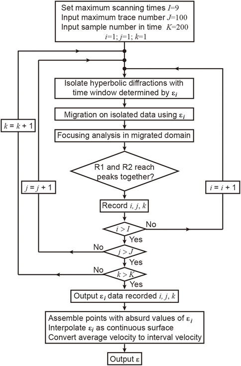
FIGURE 1. The flow chart of the proposed velocity estimation method.

The permittivity of lunar regolith and basalt blocks generally ranges from 3 to 7 (Olhoeft et al., 1975a; Heiken et al., 1991). Within this range, we apply grid searching on nine possible values. In the migrated domain, we define two parameters to evaluate the focusing effects under a given velocity, and the diffractions can be easily identified from cluttered diffractions and reflections.

2.1 Formation of hyperbolic-shape diffractions in GPR profile

The electromagnetic wave can propagate in the air and underground media. We can observe back-propagating waves of reflections on the boundary of diffractors with discontinuous dielectric properties, such as basalt blocks (Hiesinger and Head, 2006; Jolliff et al., 2006; Fa et al., 2015); similarly, we can also observe diffractions when the size of diffractor is comparable to the wavelength of electromagnetic wave. The energy of diffractions is usually smaller than that of the reflections.

We assume that each block of ejecta or rocks can be considered as a point-like diffractor since the influence of scattering body decreases with the increase of depth h₀(m); thus, the travel time of diffractions presents as a hyperbola in the GPR profile (Capineri et al., 2008; Ristic et al., 2009; Kouemou, 2010; Soldovieri and Solimene, 2010; Ding et al., 2020; Lv et al., 2020), when the GPR rover moving from x to x₀ over the diffractor at (x_0,h₀). Figure 2A illustrates the forming principle and geometric relationship of corresponding diffractions as

$\begin{array}{c}{\left({\mathit{x}}_{\mathbf{0}}-\mathit{x}\right)}^{\mathbf{2}}+{{\mathit{h}}_{\mathbf{0}}}^{\mathbf{2}}={\mathit{v}}^{\mathbf{2}}{\mathit{t}}^{\mathbf{2}},\end{array}(1)$

which can be transformed into a hyperbolic form as

$\begin{array}{c}\frac{{\mathit{t}}^{\mathbf{2}}}{{\left(\frac{{\mathit{h}}_{\mathbf{0}}}{\mathit{v}}\right)}^{\mathbf{2}}}-\frac{{\left({\mathit{x}}_{\mathbf{0}}-\mathit{x}\right)}^{\mathbf{2}}}{{{\mathit{h}}_{\mathbf{0}}}^{\mathbf{2}}}=\mathbf{1},\end{array}(2)$

where t represents the one-way travel time, v represents the average propagating velocity of electromagnetic waves. Given the location of a scatter at (x_0,h₀), the only parameter controlling the shape of hyperbola will be v. The relative magnetic permeability of most subsurface material approximately equals to 1 and the conductivity affects little during the wave propagation for high-frequency radar waves; thus, the media could be regarded as ideal dielectric and v can be calculated by (Heiken et al., 1991)

$\begin{array}{c}\mathit{v}=\frac{\mathit{c}}{\sqrt{{\mathit{\epsilon }}_{\mathit{r}}}},\end{array}(3)$

where c is the speed of light in vacuum and ԑ_r is the relative dielectric permittivity (Gold et al., 1972; Olhoeft et al., 1974; Heiken et al., 1991; Rochette et al., 2010). At the same location, for a smaller permittivity, the propagating velocity will be higher and the corresponding hyperbola will be sharper and narrower; in contrast, for a larger permittivity, the velocity will be lower and the corresponding hyperbola will be flatter and broader (Figure 2B).

FIGURE 2

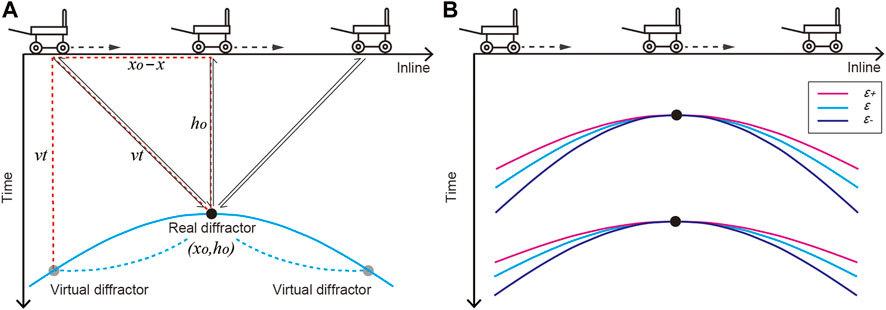
FIGURE 2. Illustration of the generation of diffractions and their isolations. (A) Mechanism of the radar observation and the forming principle of diffractions. The black lines with arrows indicate the propagation tracks of electromagnetic waves, the blue hyperbola represents the corresponding echo from the point-like diffractor in the radargram. (B) The center hyperbolas of isolating windows determined by different permittivities.

2.2 Improving signal-to-noise using migration

Migration is a common technique for imaging underground structures (Claerbout, 1985; Leuschen and Plumb, 2001; Stuart, 2003; Özdemir et al., 2014). It can numerically collect a group of diffractions into a small region around the apex if the permittivity used is close to the true one; as a result, the diffractions originally hidden by strong noises can be highlighted in the migrated domain (Li and Zhang, 2022a; Li and Zhang, 2022b). Here, we use F-K migration (Stolt, 1978), which is a direct method that is the fastest known migration technique.

We test on two simple models with strong random noises to illustrate the necessity of migration on improving signal-to-noise in the migration domain (Figure 3). We can see that the hyperbolic-shape diffractions are almost completely hidden in background noises before using migration. In contrast, the results after using migration (Stolt, 1978) show a clear peak in the wiggle along the apex of diffractions. This indicates that the weak diffractions can be extracted from the strong background noises using migration. In other words, the diffractions can be highlighted after migration and the energy peak can well indicate the location of the diffractor. With migration, we can achieve the best velocity estimation after comparing the focusing effects under different velocities. However, the actual media is far more complex with a large number of scattering objects; additionally, their diffractions mostly gather together and interfere with each other, especially for the widely existing ejecta layer on the Moon and Mars. Thus, the velocity analyses after directly using migration could not well separate these interferences. We propose to generate a series of hyperbola windows within the possible range of permittivity to isolate each group of diffractions and suppress both random noises and the interferences. The velocity analyses are performed on these isolated data thus can well handle cluttered diffractions.

FIGURE 3

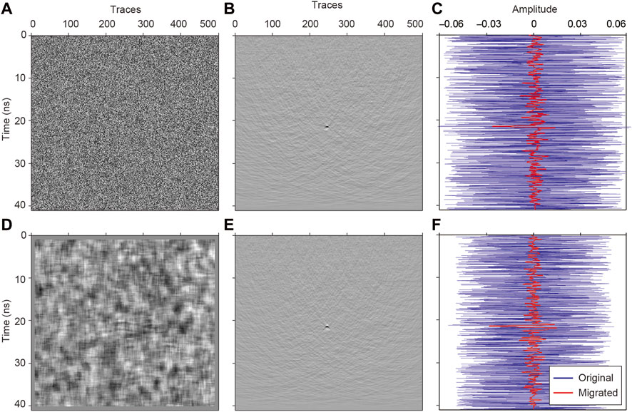
FIGURE 3. Illustration of improving the signal-to-noise ratio using migration. (A) Weak hyperbolic-shape diffractions buried in strong random noises. (B) The migration results of (A). (C) Comparison of wiggles of the one trace along the apex of diffractions: the blue curve denotes the original data shown in (A) and the red curve denotes the migrated profile shown in (B). (D–F) Another case similar to (A–C) but with a different kind of random noises shown in (D).

2.3 Diffraction isolation

The isolation of diffractions and the migration had been proven effective in reducing the above-surface diffractions (Li et al., 2021a). Traditional methods perform migration to the whole data set without isolating each group of diffractions; thus, the cluttered diffractions are still strongly interfered in the migrated domain (Carpentier et al., 2010). In contrast, we isolate the target diffractions from others in the un-migrated domain by some proper windows, which can largely avoid the influence from both adjacent diffractions and reflections, since the input data for the migration are dominated by the target diffractions and only small parts of adjacent diffractions or some segments of reflections exist. This can greatly improve the signal-to-noise ratio after applying migration to such windowed input data, compared with applying migration to the whole data; additionally, it can also improve the spatial resolution by separately analyzing each group of diffractions at a time.

According to the forming principle of diffractions, the isolation window can be automatically built up with the widen of the theoretical hyperbola. Therefore, we can build a series of hyperbola windows in different shapes at different depths using various permittivities (i.e., velocities). After analyzing some typical GPR data, we set the temporal width of the window to be 10–20 samples. These windows would be applied to isolate the diffractions from the GPR profile independently, and the surrounding noises and interferences can be well suppressed (Figure 4). In this way, the input data d can be divided into two parts: d_w(ԑi) is the isolated part within the hyperbolic window region, the shape of the hyperbolic window is under the control of permittivity ԑ_i, and the rest part is out of the window d_r = d—d_w(ԑi).

FIGURE 4

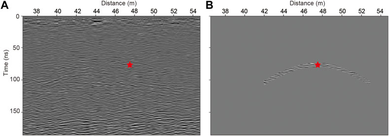
FIGURE 4. Illustration of diffraction isolation in Chang’E-4 LPR profile. (A, B) are the radar profile before and after diffraction isolation, respectively.

The main drawback of the proposed method is the huge computational cost, due to dealing with a vast number of potential diffractions independently. Fortunately, the total computational cost becomes affordable after applying a series of optimization steps. First, we apply grid searching on every 5 time steps, this can improve the efficiency greatly while preserving the shapes of diffractions; then, we apply migration within a small region instead of the whole profile, which can further reduce the computational cost; finally, we adopt a fast implementation of migration (e.g., Stolt, 1978).

2.4 Focusing analyses in migrated domain

For each group of diffractions, permittivity is the key parameter controlling the focusing effects of migration results. If the permittivity is true, the diffractions can be perfectly focused within a small region close to the true location of the diffractor; if too large, the diffractions will be under-migrated and display as a downward-opening curve with reduced spatial scale; otherwise, if too small, the diffractions will be over-migrated and display as an upward-opening curve (Figure 5) (Claerbout, 1985; Zhu et al., 1998; Li et al., 2021b). For a given group of diffractions, there must be a permittivity model with which the diffractions can be best tailored by a hyperbola window, and the migration results would be highly focused with the highest signal-to-noise ratio. In other words, for a properly-tailored group of diffractions, the permittivity can be determined once we obtain the best-focused migration results. This allows us to finely tune the velocity for each potential diffractor independently.

FIGURE 5

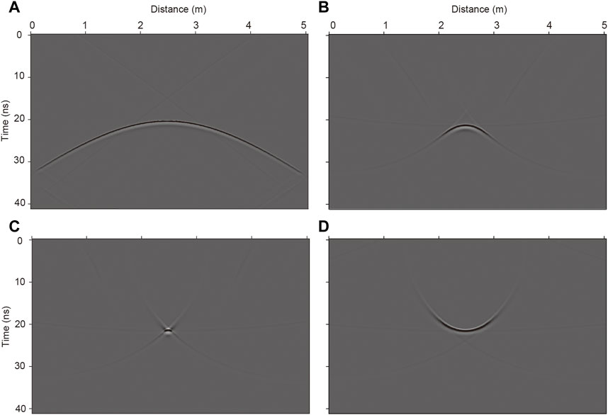
FIGURE 5. Migration results under different permittivities. (A) Hyperbolic-shape diffraction. (B–D) The corresponding migration results with the permittivity of ԑ+, ԑ, and ԑ-, respectively.

We assume that one group of diffractions is already tailored properly with a group of given windows determined by the permittivity ԑi, and A is the migrated result as below

$\begin{array}{c}\mathit{A}=\mathit{F}\mathit{K}\mathit{M}\mathit{i}\mathit{g}\left({\mathit{d}}_{\mathit{w},\mathit{ԑ}\mathit{i}}\right).\end{array}(4)$

Then we calculate the partial derivatives H_t and H_x of A in time and horizontal direction,

$\begin{array}{c}\left[{\mathit{H}}_{\mathit{t}},{\mathit{H}}_{\mathit{x}}\right]=\mathit{g}\mathit{r}\mathit{a}\mathit{d}\mathit{i}\mathit{e}\mathit{n}\mathit{t}\left(\mathit{A}\right).\end{array}(5)$

We then use the sum of H_t and H_x to represent the amplitude variation at point (t₀,x₀) in A, which can be calculated as

$\begin{array}{c}\mathit{H}\left({\mathit{t}}_{\mathbf{0}},{\mathit{x}}_{\mathbf{0}}\right)=\left|{\mathit{H}}_{\mathit{t}}\left({\mathit{t}}_{\mathbf{0}},{\mathit{x}}_{\mathbf{0}}\right)\right|+\left|{\mathit{H}}_{\mathit{x}}\left({\mathit{t}}_{\mathbf{0}},{\mathit{x}}_{\mathbf{0}}\right)\right|.\end{array}(6)$

To further quantify the amplitude variation (i.e., the focusing effects around this point under a specific permittivity), we design a gradient template around the target. We bring in a parameter P to express the focusing energy around the target:

$\begin{array}{c}\mathit{P}={\displaystyle \sum _{{\mathit{t}=\mathit{t}}_{\mathbf{0}}-\mathit{u}}^{{\mathit{t}}_{\mathbf{0}}+\mathit{u}}}{\displaystyle \sum _{{\mathit{x}=\mathit{x}}_{\mathbf{0}}-\mathit{v}}^{{\mathit{x}}_{\mathbf{0}}+\mathit{v}}}\mathit{H}\left(\mathit{t},\mathit{x}\right),\end{array}(7)$

where u and v (u > 1,v > 1) represent the side lengths of the template in time and horizontal direction, respectively. Usually, P would be greatly higher for diffractors, compared with non-diffractors. When P exceeds a certain threshold, we consider that there may be diffractors there, which require further focusing analysis. Then we introduce A,B,C,D to represent the focusing energy around the point (t₀,x₀) (Figure 6),

$\mathit{A}={\displaystyle \sum _{{\mathit{t}=\mathit{t}}_{\mathbf{0}}-\mathbf{2}\mathit{u}}^{{\mathit{t}}_{\mathbf{0}}-\mathit{u}-\mathbf{1}}}{\displaystyle \sum _{{\mathit{x}=\mathit{x}}_{\mathbf{0}}-\mathit{v}}^{{\mathit{x}}_{\mathbf{0}}+\mathit{v}}}\mathit{H}\left(\mathit{t},\mathit{x}\right),(8)$

$\mathit{B}={\displaystyle \sum _{{\mathit{t}=\mathit{t}}_{\mathbf{0}}+\mathit{u}+\mathbf{1}}^{{\mathit{t}}_{\mathbf{0}}+\mathbf{2}\mathit{u}}}{\displaystyle \sum _{{\mathit{x}=\mathit{x}}_{\mathbf{0}}-\mathit{v}}^{{\mathit{x}}_{\mathbf{0}}+\mathit{v}}}\mathit{H}\left(\mathit{t},\mathit{x}\right),(9)$

$\mathit{C}={\displaystyle \sum _{{\mathit{t}=\mathit{t}}_{\mathbf{0}}-\mathit{u}}^{{\mathit{t}}_{\mathbf{0}}+\mathit{u}}}{\displaystyle \sum _{{\mathit{x}=\mathit{x}}_{\mathbf{0}}-\mathbf{2}\mathit{v}}^{{\mathit{x}}_{\mathbf{0}}-\mathit{v}-\mathbf{1}}}\mathit{H}\left(\mathit{t},\mathit{x}\right),(10)$

$\mathit{D}={\displaystyle \sum _{{\mathit{t}=\mathit{t}}_{\mathbf{0}}-\mathit{u}}^{{\mathit{t}}_{\mathbf{0}}+\mathit{u}}}{\displaystyle \sum _{{\mathit{x}=\mathit{x}}_{\mathbf{0}}+\mathit{v}+\mathbf{1}}^{{\mathit{x}}_{\mathbf{0}}+\mathbf{2}\mathit{v}}}\mathit{H}\left(\mathit{t},\mathit{x}\right),(11)$

FIGURE 6

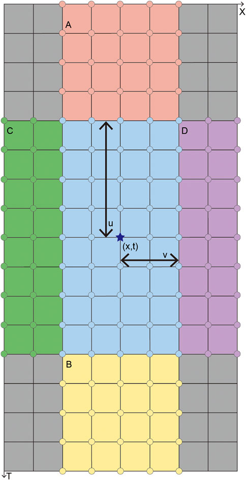
FIGURE 6. The template of energy distribution around the target (marked with the star) in migrated domain. P is the signal energy within the blue area; (A–D) represent the surrounding signal energy, drawn in pink, yellow, green and purple respectively.

In different radar profiles with different time step and spatial interval, we need to set different u and v. Figure 6 shows the template under u = 4, v = 2. For high-frequency radar profile, u is usually greater than 10 and there will be a multiple difference between u and v. Therefore, we can ignore the effects of signal energy within the gray area in Figure 6 during focus evaluation.

Then we introduce two parameters R₁ and R₂:

$\begin{array}{c}{\mathit{R}}_{\mathbf{1}}=\frac{\mathit{P}}{\mathit{P}+\mathit{A}+\mathit{B}+\mathit{C}+\mathit{D}},\end{array}(12)$

which is the gradient ratio between the amplitudes of target area (blue region in Figure 6) and all points within the template.

$\begin{array}{c}{\mathit{R}}_{\mathbf{2}}=\frac{\mathit{P}}{\mathit{A}+\mathit{B}+\mathit{C}+\mathit{D}},\end{array}(13)$

which is the gradient ratio between the amplitudes of target area and area around the target (pink, yellow, green and purple region in Figure 6). These two ratios (i.e., R₁ and R₂) can well represent the focusing effects in the migrated domain.

Here we show the R1 and R2 (Figure 7) calculated from Figures 5B–D. It is obvious that the focusing energy is the strongest under an accurate velocity model.

FIGURE 7

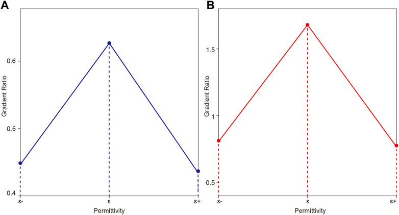
FIGURE 7. Histograms of R1[blue line in 7(A)] and R2[red line in 7(B)]. ԑ-, ԑ and ԑ+ corresponds to the over-migrated, perfectly migrated and under-migrated situation, respectively.

We argue that if there is a diffractor, there must be two maximums of R1 and R2 after comparing a series of these two ratios obtained under different permittivities. In other words, when R1 and R2 reach their maximums under the same permittivity simultaneously, this permittivity can be regarded as the best estimation; otherwise, we suppose that there is no diffractor at current point. In this way, we can locate the diffractor and estimate the corresponding permittivity simultaneously.

3 Application in lunar penetrating radar data

We hope to employ our method to a local lunar penetrating radar (LPR) profile from Chang’E-4 mission (Zhang J et al., 2021), so that we can acquire the corresponding permittivity profiles at the landing site. This can help us to better understand the structure and property of lunar subsurface material.

The LPR onboard Yutu-2 rover has two channels, with the dominant frequency of 60 MHz (Channel-1) and 500 MHz (Channel-2), respectively. We only consider the high-frequency channel, which is for detecting shallow structures. Under the dominant frequency of 500 Mhz, the diffractors with diameter over ∼15 cm would be mostly identified (Jol., 2009). The Channel-2 antennas are 30 cm over the surface, in Bowtie shape. The two receiving antennas (A and B) are close to the emitter with a distance of 15.4 cm and 31.7 cm, respectively (Fang et al., 2014). The time step of channel 2B is 0.3125 ns and spatial interval is 3.65 cm.

We first test our method with a numerical model to show its feasibility. We build a simple scattering model and perform numerical simulation with the finite-difference method (Figures 8A, B). Based on the simulated radar records, we further carry out the F-K migration and focusing analysis in the migrated domain. The scanning region (the box in Figure 8B) is between 13 ns and 17.7 ns in time, from x = 0.5 m to x = 4.25 m. Figure 8C shows that our proposed method can well locate the diffractors and derive the corresponding permittivities from the radar record.

FIGURE 8

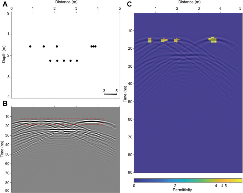
FIGURE 8. Test on a scattering model. (A) Numerical permittivity model. (B) The corresponding simulation result. (C) The result of velocity estimation.

3.1 Application in a typical group of diffractions

After confirming the feasibility of this method, we then employ it to a typical group of diffractions from the LPR profile and compare the focusing effects in the migrated domain before and after diffraction isolation. The location of the group of diffractions is marked with the red star in Figure 9.

FIGURE 9

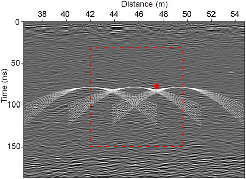
FIGURE 9. Illustration of diffraction isolation. The base map is the local LPR profile obtained by the Yutu-2 lunar rover (Zhang X et al., 2021). The star marks the location of typical diffractions used in 3.2.1. The box indicates the scanning region in 3.2.2. The hyperbolas illustrate nine rounds of diffraction isolation at three coordinate points using different permittivities.

After nine rounds of diffraction isolation and migration, we can obtain nine groups of gradient ratios R1 and R2 (Figures 10A, C). It can be seen that R1 and R2 reach their maximums simultaneously with the permittivity of 4. To be more precise, we refine the permittivity from 3.5 to 4.5 by a one-fifth interval and find that the largest ratios appear at permittivity of 3.7 (Figures 10B, D). Therefore, the best estimation of the permittivity at this point should be 3.7. Under this permittivity, we compare the focusing effects in the migrated domain with or without diffraction isolation (Figure 11). Obviously, the signal energy is better focused after using diffraction isolation, although the peak is slightly reduced compared with that before using diffraction isolation. This indicates that the diffraction isolation can well suppress the interference from noises and surrounding diffractions, which can also explain why the energy peak falls slightly. Besides, the location of the diffractor can be more accurate after diffraction isolation, as shown by the wiggles in Figure 11D.

FIGURE 10

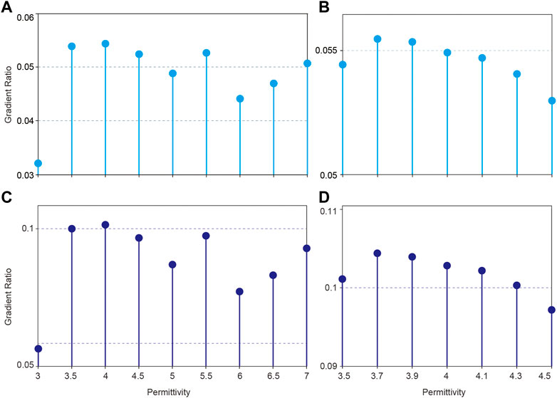
FIGURE 10. The gradient ratios histograms in typical diffraction tests. (A) and (C) list R1 and R2 calculated using different permittivities ranging from 3 to 7, respectively. (B, D) are the locally refined results between 3.5 and 4.5 of (A, C), respectively.

FIGURE 11

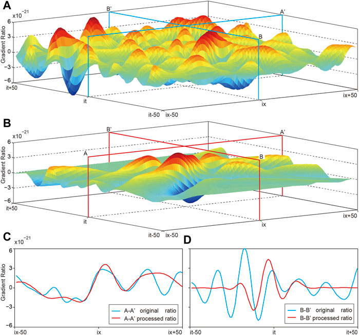
FIGURE 11. Local energy maps and slices of migration. (A, B) are energy maps with or without diffraction isolation, respectively. (it, ix) is the coordinate of the diffractor. (C) The energy slices along A-A′ shown in (A, B). (D) The energy slices along B-B′ shown in (A, B).

3.2 Application in local profile

We further apply our method to the local LPR profile. The location of the scanning region is indicated with the red dotted box in Figure 9. The original LPR data have a time step of 0.3125 ns and a spatial interval of 3.65 cm. We pick up the data every 5 time steps from traces No. 1150 to No. 1350 to save the computational cost. Comparing the gradient ratios of R1 and R2, we can pick up the diffractors while recording their corresponding permittivities. Ultimately, we can acquire a two-dimensional map of permittivity distribution using the proposed method (Figure 12).

FIGURE 12

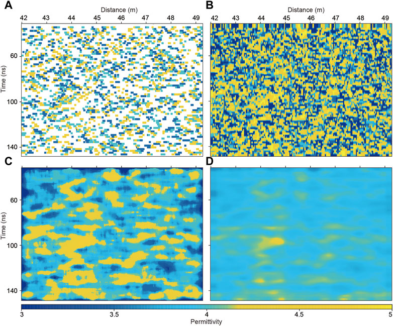
FIGURE 12. Permittivity map obtained from scattering points. (A) The scatter plot of average permittivity. (B)The interpolation result of scattering points shown in (A). (C) The median filtering result of (B). (D) The smoothed map of interval permittivity converted from (C) by Dix inversion.

The depth of the region (red box in Figure 9) is within 20 m, the permittivity is generally between 3 and 5 (Li et al., 2021b). Therefore, the permittivity beyond the range [3,5] would be absurd. We eliminate the absurd values of permittivity to avoid potential influence from few wild points (Figure 12A). Then we interpolate the permittivity profile to generate continuous velocity estimation along the whole LPR profile then apply two rounds of median filtering to smooth the interpolated results. It should be noted that the permittivity calculated above represents the depth-averaged permittivity between the surface and the diffractor, instead of the interval permittivity at a specific depth. Thus, we need to transfer it into the interval velocity with Dix inversion as follows (Dix, 1955; Bradford and Harper, 2005; Sato and Feng, 2005)

$\begin{array}{c}{\mathit{v}}_{\mathit{int},{\mathit{t}}_{\mathit{n}}}=\sqrt{\frac{{{\mathit{v}}_{\mathit{a}\mathit{v}\mathit{e},{\mathit{t}}_{\mathit{n}}}}^{\mathbf{2}}{\mathit{t}}_{\mathit{n}}-{{\mathit{v}}_{\mathit{a}\mathit{v}\mathit{e},{\mathit{t}}_{\mathit{n}-\mathbf{1}}}}^{\mathbf{2}}{\mathit{t}}_{\mathit{n}-\mathbf{1}}}{{\mathit{t}}_{\mathit{n}}-{\mathit{t}}_{\mathit{n}-\mathbf{1}}}},\end{array}(14)$

where t_n represents the time samples, v_int,_tn represents the interval velocity at the time point of t_n, and v_ave,tn represents the average velocity within time t_n, which is the average of the first n temporal pixels. Thus, the interval permittivity can be calculated point by point. Finally, the two-dimensional map of permittivity distribution can be obtained, as shown in Figure 12D. The spatial resolution can be roughly up to 30 cm, comparable to the spatial resolution of the LPR (∼30 cm). From Figures 12A, D clear increasing tendency of permittivity versus time can be seen, revealed as an expanded yellow region.

Based on this local map of permittivity distribution, we can gather more information on dielectric property by analyzing the statistical characteristics of lunar regolith. Figure 13A shows the relative permittivity scatterplot derived from the map. The permittivities vary in a similar tendency between different traces, which indicates that there is sight lateral variation along the LPR profile. Additionally, the permittivities on all points are generally ∼4 from 30 to 150 ns. The linear fitting results show a tiny increasing linear trend from 3.85 to 4.1 between 30 and 150 ns, depicted with the red line in Figure 13A. This indicates that there is almost no rapid variation of permittivity with depth. Furthermore, we calculate the mean and median of permittivity at every moment; after the reservation of only one decimal, we calculate the mode average. As shown in Figure 13B, the statistical curves reemphasize the increasing trend of permittivity versus time, and the upward tendency indicted by the mean and median permittivity are basically the same, but the curve of mean value changes more gently. It is also worth noticing that with the increasing of depth, the permittivity varies more violently. This phenomenon indicates that the heterogeneity of lunar regolith would be more obvious in deeper materials, which is generally consistent with the gardening process of shallow lunar materials (Zhang, J, et al., 2021).

FIGURE 13

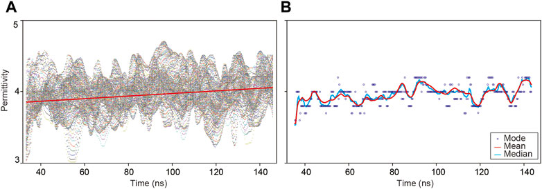
FIGURE 13. Statistical characteristics of permittivity distribution. (A) The scatterplot of permittivity, where the red line is the linear fitting result. (B) The mode, mean and median permittivities at every moment.

Another statistics and error analysis is carried out by averaging the estimated permittivities every 5 time steps, as illustrated in Figure 14A. The time points are marked with red dots, and the one standard deviation (1σ) errors within each subsection are identified with dark bars, indicting the confidence bound of our results. For instance, the average permittivity at time point t₀ is calculated with

$\begin{array}{c}{\mathit{\epsilon }}_{\mathit{r},{\mathit{t}}_{\mathbf{0}}}=\frac{{\sum }_{\mathit{i}={\mathit{t}}_{\mathbf{0}}-\mathbf{4}}^{{\mathit{t}}_{\mathbf{0}}+\mathbf{4}}{\mathit{\epsilon }}_{\mathit{r},\mathit{i}}}{\mathbf{9}},t_0=\mathrm{5,10,15}\dots \end{array}(15)$

FIGURE 14

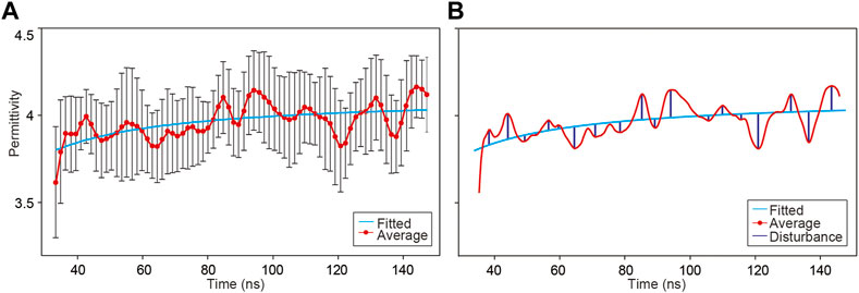
FIGURE 14. Permittivity distribution along time. (A) The red line with dots and the black bars represent the average permittivity and one standard deviation every 5 time steps, respectively. (B) The red line is the average permittivity at every moment, and the blue curve represents the fitting result. The vertical bars represent the perturbation of peaks and valleys.

This graph provides a new sight for analyzing the permittivity distribution. Averaging the permittivity helps to limit the influence of some singular permittivity values while retaining the local characteristics on the overall trend, which is beneficial to summarize the relationship between permittivity and travel time.

With the estimated permittivity at a certain travel time, we can extract a relationship by curve fitting as

$\begin{array}{c}{\mathit{\epsilon }}_{\mathit{r}}=\frac{\mathbf{4.1}\mathit{t}+\mathbf{16.41}}{\mathit{t}+\mathbf{6.884}},\end{array}(16)$

where t is the travel time (ns), ${\epsilon }_r$ is the relative permittivity. Consistent with previous studies, the statistical regulation shows an increasing trend of permittivity versus depth, indicating that the relative permittivity of lunar subsurface materials is in strong positive correlations with depth. The red curve in Figure 14B represents the averaged permittivity at every moment, and the blue curve is the fitted relationship. With these fitting results, we can analyze the degree of permittivity variation within this region. The peaks and valleys at time point t_j are collected and the root mean square local permittivity perturbation ξ can be calculated with

$\begin{array}{c}\mathit{\xi }={\displaystyle \sum _{\mathit{j}=\mathbf{1}}^{\mathit{N}}}\frac{\left|{\mathit{\epsilon }}_{\mathit{r},{\mathit{t}}_{\mathit{j}}}-{\mathit{\epsilon }}_{\mathit{f}\mathit{i}\mathit{t},{\mathit{t}}_{\mathit{j}}}\right|}{\mathit{N}\bullet {\mathit{\epsilon }}_{\mathit{f}\mathit{i}\mathit{t},{\mathit{t}}_{\mathit{j}}}},\end{array}(17)$

where N is the number of peaks and valleys, ${\epsilon }_{r,t_j}$ and ${\epsilon }_{fit,t_j}$ is the averaged relative permittivity and the fitted one, respectively. The local permittivity perturbation ξ is estimated to be ∼2.3%, which is consistent with 3% obtained by the simulated results (Zhang, X., et al., 2021). This verified that the lunar regolith at the Chang’E-4 landing area can be well described by self-organization random models.

4 Discussion

Compared with the existing methods, our method has some unique advantages. The hyperbolic-fitting method requires that the diffractions should be in well-formed and distinguishable hyperbolic shape, which is difficult to achieve in practice; additionally, the traditional migration method can not suppress the surrounding noises and interferences in the focusing analysis due to working on the whole profile, which may lead to large errors. Our method combines the advantage of hyperbolic fitting and migration; thus, it can help to estimate the relative permittivity more precisely and effectively, especially for complex materials. Besides, the spatial resolution of our method is to that of the LPR payload, which can help to better recognize and delineate the abnormal bodies in subsurface materials.

Limited by the computation cost, our method is only applied in shallow part within 12 m in depth and within ∼7 m in distance; however, the statistical characteristics extracted from this local area should be universal to the Chang’E-4 landing area along the rover’s track. The map of permittivity distribution shows that there is an abnormal high-permittivity region existing in the map at ∼100 ns? We suppose that small basaltic or ejecta blocks may gather there. Besides, we can notice that the permittivity becomes larger and varies severer with the increasing depth. This indicates that there is a strong positive correlation between the permittivity of lunar subsurface materials and depth, and the heterogeneity of lunar regolith is more obvious in deeper materials. The increasing tendency of permittivity with depth is consistent with former studies (Heiken et al., 1991). We suppose this is probably because of more blocks or larger grain size of deeper materials.

5 Conclusion

We propose a migration-based method to estimate the relative permittivity of subsurface materials from the ground penetrating radar data, including three steps: diffraction isolation, migration, and focusing analysis. Single point test shows that diffraction isolation can help to improve the reliability of migration and is a prerequisite for accurate focusing analysis in the migrated domain. Numerical experiments show that the proposed method is robust and effective for permittivity estimation, especially in the presence of strong noises and cluttered diffractions. The spatial resolution is higher than that of the existing methods due to the application of diffraction isolation and migration; thus, we can pick up a great number of diffractors, which is helpful to construct a continuous velocity profile in depth. The permittivity at the Chang’E-4 landing area is estimated to be ∼4 within 12 m, ranging from 3.5 to 4.2. Additionally, the local perturbation of the permittivity is ∼2.3%, which is consistent with that (∼3%) obtained by numerical simulations using self-organization random models. This suggests that the lunar regolith at Chang’E-4 landing area is mature and can be well described by the self-organization random models.

Data availability statement

Publicly available datasets were analyzed in this study. This data can be found here: https://moon.bao.ac.cn/ce5web /searchOrder_dataSearchData.search.

Author contributions

Conceptualization: WL and JZ; Methodology: WL; Supervision: JZ; Writing—Original draft: WL and JZ; Writing—Review and editing: WL and JZ. All authors contributed to the article and approved the submitted version.

Funding

This research was supported by the National Natural Science Foundation of China (41941002), Key Research Program of the Institute of Geology and Geophysics, CAS (IGGCAS-202203), and Key Research Program of the Chinese Academy of Sciences (ZDBS-SSWTLC001). JZ was also supported by Foundation for Excellent Member of the Youth Innovation Promotion Association, Chinese Academy of Sciences (2016).

Acknowledgments

We thank the Supercomputing Laboratory of Institute of Geology and Geophysics, Chinese Academy of Sciences (IGGCAS) for providing computing resources.

Conflict of interest

The authors declare that the research was conducted in the absence of any commercial or financial relationships that could be construed as a potential conflict of interest.

Publisher’s note

All claims expressed in this article are solely those of the authors and do not necessarily represent those of their affiliated organizations, or those of the publisher, the editors and the reviewers. Any product that may be evaluated in this article, or claim that may be made by its manufacturer, is not guaranteed or endorsed by the publisher.

References

Boisson, J., Heggy, E., Clifford, S. M., Frigeri, A., Plaut, J. J., Farrell, W. M., et al. (2009). Sounding the subsurface of Athabasca Valles using MARSIS radar data: Exploring the volcanic and fluvial hypotheses for the origin of the rafted plate terrain. J. Geophys. Res. Planets114 (E8). doi:10.1029/2008JE003299

CrossRef Full Text | Google Scholar

Bradford, J. H., and Harper, J. T. (2005). Wave field migration as a tool for estimating spatially continuous radar velocity and water content in glaciers. Geophys. Res. Lett.32 (8), L08502. doi:10.1029/2004GL021770

CrossRef Full Text | Google Scholar

Capineri, L., Daniels, D. J., Falorni, P., Lopera, O. L., and Windsor, C. G. (2008). Estimation of relative permittivity of shallow soils by using the ground penetrating radar response from different buried targets. Prog. Electromagn. Res. Lett.2, 63–71. doi:10.2528/PIERL07122803

CrossRef Full Text | Google Scholar

Carpentier, S. F., Horstmeyer, H., Green, A. G., Doetsch, J., and Coscia, I. (2010). Semiauto-mated suppression of above-surface diffractions in GPR data. Geophysics75 (6), J43–J50. doi:10.1190/1.3497360

CrossRef Full Text | Google Scholar

Carrier, W. D., Olhoeft, G. R., and Mendell, W. (1991). Physical properties of the lunar surface. Lunar Sourceb., 475–594.

Google Scholar

Claerbout, J. F. (1985). Imaging the earth's interior. Oxford: Blackwell scientific publications.

Google Scholar

Dai, S., Su, Y., Yuan, X., Feng, J., and Xing, S. (2014). Lunar regolith structure model and echo simulation for Lunar Penetrating Radar. IEEE, Proceedings of the 15th International Conference on Ground Penetrating Radar. July 4, 2014, Belgium, IEEE.

Ding, C., Li, C., Xiao, Z., Su, Y., Xing, S., Wang, Y., et al. (2020). Layering structures in the porous material beneath the Chang'e-3 landing site. Earth Space Sci.7, e2019EA000862. doi:10.1029/2019EA000862

CrossRef Full Text | Google Scholar

Dix, C. H. (1955). Seismic velocities from surface measurements. Geophysics20 (1), 68–86. doi:10.1190/1.1438126

CrossRef Full Text | Google Scholar

Dong, Z., Fang, G., Zhao, D., Zhou, B., Gao, Y., and Ji, Y. (2020). Dielectric properties of lunar subsurface materials. Geophys. Res. Lett.47 (22), e2020GL089264. doi:10.1029/2020GL089264

CrossRef Full Text | Google Scholar

Economou, N., Vafidis, A., Bano, M., Hamdan, H., and Ortega-Ramirez, J. (2020). Ground-penetrating radar data diffraction focusing without a velocity model. Geophysics85 (3), H13–H24. doi:10.1190/geo2019-0101.1

CrossRef Full Text | Google Scholar

Fa, W., Zhu, M., Liu, T., and Plescia, J. (2015). Regolith stratigraphy at the Chang'E-3 landing site as seen by lunar penetrating radar. Geophys. Res. Lett.42 (23), 10179–10187. doi:10.1002/2015gl066537

CrossRef Full Text | Google Scholar

Fang, G., Zhou, B., Ji, Y., Zhang, Q., Shen, S., Li, Y., et al. (2014). Lunar penetrating radar onboard the chang'e-3 mission. Res. astronomy astrophysics14 (12), 1607–1622. doi:10.1088/1674-4527/14/12/009

CrossRef Full Text | Google Scholar

Feng, J., Su, Y., Li, C., Dai, S., Xing, S., and Xiao, Y. (2019). An imaging method for Chang'e5 Lunar Regolith Penetrating Radar. Planet. Space Sci.167 (MAR.), 9–16. doi:10.1016/j.pss.2019.01.008

CrossRef Full Text | Google Scholar

Fomel, S., Landa, E., and Taner, M. T. (2007). Poststack velocity analysis by separation and imaging of seismic diffractions. Geophysics72 (6), U89–U94. doi:10.1190/1.2781533

CrossRef Full Text | Google Scholar

Fomel, S. (2003a). Time-migration velocity analysis by velocity continuation. Geophysics68 (5), 1662–1672. doi:10.1190/1.1620640

CrossRef Full Text | Google Scholar

Fomel, S. (2003b). Velocity continuation and the anatomy of residual prestack time migration. Geophysics68 (5), 1650–1661. doi:10.1190/1.1620639

CrossRef Full Text | Google Scholar

Giannakis, I., Zhou, F., Warren, C., and Giannopoulos, A. (2021). Inferring the shallow layered structure at the chang'e-4 landing site: A novel interpretation approach using lunar penetrating radar. Geophys. Res. Lettdoi:10.1002/essoar.10506249.1

CrossRef Full Text | Google Scholar

Gold, T., Bilson, E., and Yerbury, M. (1972). Grain size analysis, optical reflectivity measurements, and determination of high-frequency electrical properties for Apollo 14 lunar samples. Lunar Planet. Sci. Conf. Proc.

Google Scholar

Hamran, S. E., Paige, D. A., Amundsen, H., Berger, T., Yan, M. J., Carter, L., et al. (2020). Radar imager for Mars' subsurface experiment—rimfax. Space Sci. Rev.216 (128), 128. doi:10.1007/s11214-020-00740-4

CrossRef Full Text | Google Scholar

Heiken, G. H., Vaniman, D. T., and French, B. M. (1991). Lunar Sourcebook, a user's guide to the Moon. Houston, Texas. Cambridge University Press.

Google Scholar

Hiesinger, H., and Head, J. W. (2006). New views of lunar geoscience: An introduction and overview. Rev. mineralogy Geochem.60 (1), 1–81. doi:10.2138/rmg.2006.60.1

CrossRef Full Text | Google Scholar

Hu, J., Schuster, G. T., and Valasek, P. A. (2001). Poststack migration deconvolution. Geophysics66 (3), 939–952. doi:10.1190/1.1444984

CrossRef Full Text | Google Scholar

Jol, H. (2009). Ground penetrating radar: Theory and applications. Germany: Elsevier Science.

Google Scholar

Jolliff, B. L., Wieczorek, M. A., Shearer, C. K., and Neal, C. R. (2006). New views of the Moon. Beijing: Walter de Gruyter GmbH and Co KG. doi:10.2138/rmg.2006.60.0

CrossRef Full Text | Google Scholar

Jordan, R., Picardi, G., Plaut, J., Wheeler, K., Kirchner, D., Safaeinili, A., et al. (2009). The Mars express MARSIS sounder instrument. Planet. Space Sci.57 (14–15), 1975–1986. doi:10.1016/j.pss.2009.09.016

CrossRef Full Text | Google Scholar

Kouemou, G. (2010). Radar technology.GermanyBoD–Books on Demand.

Google Scholar

Leong, Z. X., and Zhu, T. (2021). Direct velocity inversion of ground penetrating radar data using GPRNet. J. Geophys. Res. Solid Earth126, e2020JB021047. doi:10.1029/2020JB021047

CrossRef Full Text | Google Scholar

Leuschen, C. J., and Plumb, R. G. (2001). A matched-filter-based reverse-time migration algorithm for ground-penetrating radar data. IEEE Trans. Geoscience Remote Sens.39 (5), 929–936. doi:10.1109/36.921410

CrossRef Full Text | Google Scholar

Li, C., Lin, Y., Lv, W., and Zhang, J. (2021b). Eliminating above-surface diffractions from ground-penetrating radar data using iterative Stolt migration. Geophysics86 (1), H1–H11. H1–H11. doi:10.1190/GEO2019-0796.1

CrossRef Full Text | Google Scholar

Li, C., Zhang, J., Loxas, M., and Sharma, P. (2021a). Hemosiderotic dermatofibroma mimicking melanoma: A case report and review of the literature. Remote Sens.13, 1387–1392. doi:10.3390/rs13071387

CrossRef Full Text | Google Scholar

Li, C., and Zhang, J. (2022a). Preserving signal during random noise attenuation through migration enhancement and local orthogonalization. Geophysics87, V451–V466. doi:10.1190/geo2021-0385.1

CrossRef Full Text | Google Scholar

Li, C., and Zhang, J. (2022b). Wavefield separation using irreversible-migration filtering. Geophysics87 (3), A43–A48. A43–A48. doi:10.1190/GEO2021-0607.1

CrossRef Full Text | Google Scholar

Li, C., Zheng, Y., Wang, X., Zhang, J., Wang, Y., Chen, L., et al. (2022). Layered subsurface in utopia basin of Mars revealed by zhurong rover radar. Nature610, 308–312. doi:10.1038/s41586-022-05147-5

PubMed Abstract | CrossRef Full Text | Google Scholar

Li, J., Zeng, Z., Liu, C., Huai, N., and Wang, K. (2017). A study on lunar regolith quantitative random model and lunar penetrating radar parameter inversion. IEEE Geoscience Remote Sens. Lett.14 (11), 1953–1957. doi:10.1109/LGRS.-2017.2743618

CrossRef Full Text | Google Scholar

Lv, W., Li, C., Song, H., Zhang, J., and Lin, Y. (2020). Comparative analysis of reflection characteristics of lunar penetrating radar data using numerical simulations. Icarus350, 113896. doi:10.1016/j.icarus.2020.113896

CrossRef Full Text | Google Scholar

Olhoeft, G., Frisillo, A., Strangway, D., and Sharpe, H. (1974). Temperature dependence of electrical conductivity and lunar temperatures. moon9 (1-2), 79–87. doi:10.1007/bf00565394

CrossRef Full Text | Google Scholar

Olhoeft, G. R., and Strangway, D. W. (1975b). Dielectric properties of the first 100 meters of the Moon. Earth Planet. Sci. Lett.24, 394–404. doi:10.1016/0012821x(75)90146-6

CrossRef Full Text | Google Scholar

Olhoeft, G., Strangway, D., and Pearce, G. (1975a). Effects of water on electrical properties of lunar fines. Proc. Lunar Sci. Conf. 6th, 3333–3342.

Google Scholar

Oudart, N., Ciarletti, V., Le Gall, A., Mastrogiuseppe, M., Hervé, Y., Benedix, W. S., et al. (2021). Range resolution enhancement of WISDOM/ExoMars radar soundings by the Bandwidth Extrapolation technique: Validation and application to field campaign measurements. Planet. Space Sci.197, 105173. doi:10.1016/j.pss.2021.105173

CrossRef Full Text | Google Scholar

Özdemir, C., Demirci, Ş., Yiğit, E., and Yilmaz, B. (2014). A review on migration methods in B-scan ground penetrating radar imaging. Math. Problems Eng.2014, 1–16. doi:10.1155/2014/280738

CrossRef Full Text | Google Scholar

Reshef, M., and Landa, E. (2009). Post-stack velocity analysis in the dip-angle domain using diffractions. Geophys. Prospect.57 (5), 811–821. doi:10.1111/j.1365-2478.2008.00773.x

CrossRef Full Text | Google Scholar

Ristic, A. V., Petrovacki, D., and Govedarica, M. (2009). A new method to simultaneously estimate the radius of a cylindrical object and the wave propagation velocity from GPR data. ComputersandGeosciences35 (8), 1620–1630. doi:10.1016/j.cageo.2009.01.003

CrossRef Full Text | Google Scholar

Rochette, P., Gattacceca, J., Ivanov, A., Nazarov, M., and Bezaeva, N. (2010). Magnetic properties of lunar materials: Meteorites, Luna and Apollo returned samples. Earth Planet. Sci. Lett.292 (3–4), 383–391. doi:10.1016/j.epsl.2010.02.007

CrossRef Full Text | Google Scholar

Sato, M., and Feng, X. (2005). GPR migration algorithm for landmines buried in inhomogeneous soil. IEEE Antennas and Propagation Society International Symposium.

Google Scholar

Sava, P. C., Biondi, B., and Etgen, J. (2005). Wave-equation migration velocity analysis by focusing diffractions and reflections. Geophysics, 70(3), U19–U27. doi:10.1190/1.1925749

CrossRef Full Text | Google Scholar

Schroeder, D. M., Dowdeswell, J. A., Siegert, M. J., Bingham, R. G., Chu, W., MacKie, E. J., et al. (2019). Multidecadal observations of the Antarctic ice sheet from restored analog radar records. Proc. Natl. Acad. Sci.116 (38), 18867–18873. doi:10.1073/pnas.1821646116

PubMed Abstract | CrossRef Full Text | Google Scholar

Soldovieri, F., and Solimene, R. (2010). Ground penetrating radar subsurface imaging of buried objects. Tech.

CrossRef Full Text | Google Scholar

Song, H., Li, C., Zhang, J., Wu, X., Liu, Y., and Zou, Y. (2021). Rock location and property analysis of lunar regolith at Chang’E-4 landing site based on local correlation and semblance analysis. Remote Sens.13 (1), 48. doi:10.3390/rs13010048

CrossRef Full Text | Google Scholar

Stolt, R. H. (1978). Migration by fourier transform. Geophysics43 (1), 23–48. doi:10.1190/1.1440826

CrossRef Full Text | Google Scholar

Stuart, G. (2003). Characterization of englacial channels by ground-penetrating radar: An example from austre Brøggerbreen, Svalbard. J. Geophys. Res. Solid Earth108 (B11), 2525. doi:10.1029/2003JB002435

CrossRef Full Text | Google Scholar

Su, Y., Fang, G. Y., Feng, J. Q., Xing, S. G., Ji, Y. C., Zhou, B., et al. (2014). Data processing and initial results of Chang'e-3 lunar penetrating radar. Res. Astronomy Astrophysics14 (12), 1623–1632. doi:10.1088/1674–4527/14/12/010

CrossRef Full Text | Google Scholar

Xiao, L., Zhu, P., Fang, G., Xiao, Z., Zou, Y., Zhao, J., et al. (2015). A young multilayered terrane of the northern Mare Imbrium revealed by Chang’E-3 mission. Science347 (6227), 1226–1229. doi:10.1126/science.1259866

PubMed Abstract | CrossRef Full Text | Google Scholar

Yilmaz, Ö. (2001). Seismic data analysis: Processing, inversion, and interpretation of seismic data. fm: Society of exploration geophysicists. doi:10.1190/1.9781560801580

CrossRef Full Text | Google Scholar

Yuan, H., Montazeri, M., Looms, M. C., and Nielsen, L. (2019). Diffraction imaging of ground-penetrating radar data. Geophysics84 (3), H1–H12. doi:10.1190/geo2018-0269.1

CrossRef Full Text | Google Scholar

Zhang, H., Zheng, L., Su, Y., Fang, G., Zhou, B., Feng, J., et al. (2014). Performance evaluation of lunar penetrating radar onboard the rover of CE-3 probe based on results from ground experiments. Res. Astronomy Astrophysics14 (12), 1633–1641. doi:10.1088/1674–4527/14/12/011

CrossRef Full Text | Google Scholar

Zhang, J., Yang, W., Hu, S., Lin, Y., Fang, G., Li, C., et al. (2015). Volcanic history of the imbrium basin: A close-up view from the lunar rover Yutu. Proc. Natl. Acad. Sci.112 (17), 5342–5347. doi:10.1073/pnas.1503082112

PubMed Abstract | CrossRef Full Text | Google Scholar

Zhang, J., Zhou, B., Lin, Y., Zhu, M., Song, H., Dong, Z., et al. (2021). Lunar regolith and substructure at Chang’E-4 landing site in South Pole-Aitken basin. Nat. Astron.5, 25–30. doi:10.1038/s41550-020-1197-x

CrossRef Full Text | Google Scholar

Zhang, X., Lv, W., Zhang, l., Zhang, J., Lin, Y., and Yao, Z. (2021). Self-organization characteristics of lunar regolith inferred by Yutu-2 lunar penetrating radar. Remote Sens.13, 3017. doi:10.3390/rs13153017

CrossRef Full Text | Google Scholar

Zhou, B., Shen, S., Lu, W., Liu, Q., Tang, C., Li, S., et al. (2020). The Mars rover subsurface penetrating radar onboard China's Mars 2020 mission. Earth Planet. Phys.4 (4), 1–10. doi:10.26464/epp2020054

CrossRef Full Text | Google Scholar

Zhu, J., Lines, L., and Gray, S. (1998). Smiles and frowns in migration/velocity analysis. Geophysics63 (4), 1200–1209. doi:10.1190/1.1444420

CrossRef Full Text | Google Scholar