A comparison of FORMOSAT-3/COSMIC radio occultation and ionosonde measurements in sporadic E detection over mid- and low-latitude regions

1 Introduction

Thin layers of enhanced electron density compared to the background ionization in the ionosphere’s E region are referred to as sporadic E and abbreviated as Es (Whitehead, 1989; Mathews, 1998; Wu et al., 2005; Haldoupis, 2011). The Es layer is mainly known as a daytime and summer hemisphere phenomenon with higher occurrence rate at mid and low latitudes (Haldoupis et al., 2007; Christakis et al., 2009; Arras et al., 2010; Haldoupis, 2012).

Whitehead (1961) and Axford and Cunnold (1966) proposed that Es layers are formed by the wind shear mechanism. In subsequent studies, the wind shear theory has been confirmed as the physical mechanism responsible for the mid-latitude Es layer formation process (Whitehead, 1989; Haldoupis & Pancheva, 2002; Haldoupis, 2011; Yamazaki et al., 2022). According to the wind shear theory, metallic ions in the ionosphere dynamo region converge to thin layers of ionization by the vertical shears of neutral wind, mainly produced by atmospheric tides (Haldoupis, 2012; Chu et al., 2014; Shinagawa et al., 2017; Qiu et al., 2019; Sobhkhiz-Miandehi et al., 2022).

Es has been subject to many studies since the mid-twentieth century (Whitehead, 1961; 1970; 1989; Macleod, 1966) due to its potential disturbances on the radio signals in communication and navigation systems. Strong vertical electron density gradients of Es layers can cause severe radio wave propagation disruption and will directly influence the accuracy and reliability of satellite communication and navigation systems (Arras, 2010).

For many years, most of the observational studies of Es were performed using ionosonde recordings; there were also several investigations based on incoherent and coherent scatter radars and some through in situ measurements with rockets. These techniques have been documented in several review papers (Matsushita, 1962; Whitehead, 1989; Mathews, 1998; Haldoupis, 2011). However, with the development of the GPS radio occultation technique over the past two decades, satellite observations have become an increasingly popular tool for studying Es layers due to their ability to provide global data coverage (Igarashi et al., 2001; Wu et al., 2005; Arras et al., 2008).

First, Es occurrence global maps were introduced in the early 60s based on ionosonde measurements (Taguchi, 1961; Leighton et al., 1962). Reddy and Matsushita (1969) studied Es layers at mid and low latitudes utilizing the ionosonde to establish a more detailed understanding of temporal and latitudinal variations of them. Subsequently, until the 1990s, numerous studies typically focused on examining the diurnal and seasonal variations of Es by utilizing ionosonde observations (Axford & Cunnold, 1966; Harris and Taur, 1972; Chandra and Rastogi, 1975; Saksena, 1976; MacDougall, 1978; Baggaley, 1984).

In the 2000s, scientists started using GPS radio occultation measurements to study lower ionospheric irregularities such as Es. For the first time, Igarashi et al. (2001) conducted a study that used less than 6,000 occultation GPS/MET radio data from 1995 to examine the seasonal dependency of Es layers. Wickert et al. (2004) suggested that fluctuations in the CHAMP radio occultation amplitude data can be associated with ionospheric scintillations. Furthermore, Wu et al. (2005) presented a global climatology of the phase variances and signal-to-noise ratio (SNR) fluctuations using approximately 6000 GPS/CHAMP occultation in the E region.

Since the release of radio occultation measurements from FORMOSAT-3/COSMIC in the summer of 2006, our understanding of Es has significantly improved due to its global coverage. Arras et al. (2008) published the first Es occurrence rate global climatology using CHAMP, GRACE, and FORMOSAT-3/COSMIC radio occultation, which had a significantly better spatial and temporal resolution compared to previous studies. Subsequently, studies investigating Es on a global scale have been primarily based on radio occultation measurements (Wu et al., 2005; Chu et al., 2014; Qiu et al., 2019; Yu et al., 2019; Luo et al., 2021; Arras et al., 2022), while some literature has used ionosonde observations locally as an evaluation tool for their satellite-based investigations (Gooch et al., 2020; Carmona et al., 2022; Gan et al., 2022; Yu et al., 2022). Recently, Gan et al. (2022) used radio occultation data from the new China Seismo-Electromagnetic Satellite mission to derive Es events and used Wuhan ionosonde observations to assess the reliability of their research. Carmona et al. (2022) compared different GPS radio occultation techniques with ionosonde measurements over an 8-year period in order to identify the most accurate method for detecting Es occurrences using radio occultation data. Gooch et al. (2020) presented a global comparison of the intensity and height of mid-latitude and equatorial Es layers derived from FORMOSAT-3/COSMIC radio occultation and digital ionosonde measurements. All of these studies found a qualitative agreement between their satellite dataset and ionosonde measurements of the Es layer. However, they were limited by observations at a single ionosonde location during a restricted time frame and did not account for the diurnal, seasonal, and spatial dependence of Es layer detectability with satellite and ground-based techniques. In this paper, we have conducted a multi-year comparison of the mid- and low-latitude Es events recorded by an ionosonde ground-based technique to those observed using the satellite radio occultation method. Moreover, the diurnal, seasonal, and local dependence of the agreement between the two methods has been examined.

2 Data and methodology

2.1 Ionosonde

For decades, an ionosonde has remained the most commonly utilized instrument in ionospheric studies. Basically, an ionosonde transmits signals with increasing frequency from 0.1 to 30 MHz, and the frequency at which the initial signal is reflected completely will be recorded; it is known as critical frequency (fc). By measuring the frequency and reflection time of the transmitted signal, the electron density of the reflection point and the height of the ionization layer will be obtained. Two common frequency parameters used in Es layer studies are “foEs” and “fbEs.” foEs represents the ordinary mode peak frequency of the layer, and technically, it shows the maximum frequency at which an Es layer will reflect a signal transmitted by the ionosonde. fbEs corresponds to the peak blanketing frequency of Es, representing the frequency at which the reflections from higher layers appear (Piggott, 1972; Wakai et al., 1987; Merriman et al., 2021).

In this study, we used the Digital Ionogram Database (DIDBase) repository of the Lowell Global Ionospheric Radio Observatory (GIRO) Data Center (Reinisch and Galkin, 2011). The Es events were derived from the ionograms manually. Six stations, as illustrated in Figure 1, were selected to encompass the mid- and low-latitude areas of both hemispheres across various longitudes. Additionally, the selection of ionosonde stations took into consideration the availability of sufficient data during the period when we have access to radio occultation observations. The ionosonde measurements used in this study were recorded with a time resolution of 15 min.

FIGURE 1

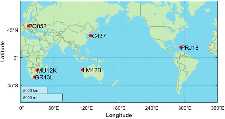
FIGURE 1. Map of the ionosonde stations.

Table 1 provides details about the stations under investigation. Pruhonice and I-Cheon are situated at the mid-latitude region of the Northern Hemisphere, while Grahamstown serves as a representative of the mid-latitude region in the Southern Hemisphere. The Ramey station is located in the low-latitude region of the Northern Hemisphere, while the Madimbo and Learmonth stations are in the low-latitude region of the Southern Hemisphere, as investigated in our study.

TABLE 1

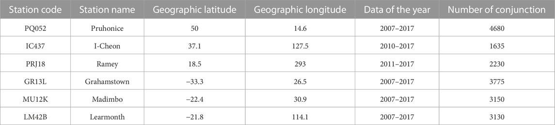
TABLE 1. List of ionosonde stations.

2.2 FORMOSAT-3/COSMIC radio occultation

The GPS radio occultation technique is principally based on receiving GPS dual-frequency signals traveling through the atmosphere by a low earth-orbiting (LEO) satellite. GPS signals are bent on their way through the atmosphere due to atmospheric refraction. The angle of this bending is the key observation and contains information on several atmospheric parameters, including electron density, temperature, pressure, and water vapor profiles (Hajj et al., 2002). The main advantages of radio occultation over ground-based techniques are its global coverage of atmospheric parameters and high spatial resolution. Nevertheless, the temporal resolution of radio occultation data is not as optimal as ground-based measurements at a specific location (Arras, 2010).

FORMOSAT-3/COSMIC stands for FORMOsa SATellite mission–3/Constellation Observing System for Meteorology, Ionosphere, and Climate. This American–Taiwanese mission has a constellation of six LEO satellites, which receive data from setting and rising occultations. Signal phase differences, ionospheric excess phase, and SNR values are three parameters that have been used in the literature to detect Es layers (Igarashi et al., 2001; Wu et al., 2005; Arras, 2010). According to the work of Arras (2010), utilizing L1 signal SNR for Es detection offers advantages such as direct access to SNR profiles without the need for data smoothing, avoidance of noisy L2 data, and simplified analysis using raw GNSS L1 data, reducing errors in data analysis. This study relies on the Es detection method presented by Arras and Wickert (2018). They derived Es events from the SNR profiles of the GPS L1 signal of the 50 Hz level 1b atmPhs data product archived by the COSMIC Data Analysis and Archive Center (CDAAC). Empirical thresholds for SNR values were established by Arras and Wickert (2018) through manual examination of radio occultation profiles. SNR values were calculated at 2 km moving intervals and utilized to identify signal scintillations with an SNR standard deviation exceeding 0.2, provided that these large standard deviation values were concentrated within an altitude range of less than 10 km. This altitude criterion of 10 km was incorporated into the Es detection process to distinguish Es events from signal disruptions caused by technical issues or upper-layer effects like spread F from the ionospheric F layer. As SNR values are affected by the viewing angle of the GNSS satellite in relation to the LEO satellite antenna, normalized SNR values were used instead of SNR. This was carried out through the following formula (Arras, 2010):

$SN{R}^{\prime }\left(i\right)=\frac{SNR\left(i\right)}{\overline{SNR}},$

where $SN{R}^{\prime }\left(i\right)$ is the normalized $SNR$ at profile i and $\overline{SNR}$ is the average SNR value of all profiles.

According to Wu et al. (2005), the Es layer typically extends horizontally for hundreds of kilometers, with a thickness of a few kilometers. Considering that approximately 1° corresponds to 100 km, a 2° latitude × 5° longitude grid was implemented around each ionosonde station to ensure simultaneous observations between ground-based and GPS radio occultation techniques. This grid size was intentionally chosen to be smaller than the average dimensions of the Es layer. Following the identification of all radio occultation crossings within a time difference of less than 15 min, all synchronous ionograms were inspected manually to find Es events. The 15-min time interval was selected based on the sounding frequency of the ionosonde stations.

3 Results

Through a comparison of ionosonde recordings and GNSS radio occultation profiles, the results demonstrate that the agreement between the two methods in detecting Es layers ranged from 60% to 80% at different stations. We identified four possible outcomes when comparing the detection of Es layers using ionograms and GPS SNR profiles: 1) both methods detected the Es layer, 2) the Es layer was identified in ionograms but not in GPS SNR profiles, 3) GPS SNR profiles indicated the presence of an Es layer, but no signal reflection was recorded via the ionosonde in the corresponding epoch in the E region, and 4) neither method recorded the occurrence of an Es layer. To gain a more comprehensive understanding of the distribution of these four types across all conjunction data points, we provided a confusion matrix of approximately 9,000 mid-latitude observations, presented in Table 2. It is important to note that in this paper, the notation Es = 1 signifies the presence of the Es layer, while Es = 0 denotes its absence. Furthermore, the detection of the Es layer using a specific technique is shown on the index. For instance, Es_ionogram = 1 indicates that the Es layer has been detected using an ionosonde.

TABLE 2

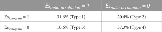
TABLE 2. Confusion matrix of ∼9,000 conjunction data points of ionograms and radio occultation profiles.

Table 2 illustrates that the detection of Es layers is in agreement between ionograms and radio occultation observations in approximately 70% of the data points (summation of Type 1 and Type 4). The remaining observations are divided into two categories: Type 2 and Type 3, which account for approximately 30% of the observations. Type 2 represents approximately 65% of the remaining data, where the Es layer is observed in ionograms but not in radio occultation profiles. Conversely, Type 3, which represents almost 35% of the remaining observations, indicates the presence of an Es layer according to satellite data, but no signal reflection was recorded in ionograms. Examining similar tables for each station from 2007 to 2017, we observed that the disagreement rate between the two methods (summation of Type 2 and Type 3) varies between 20% and a maximum of 40%.

Figure 2 showcases two illustrative examples, specifically Type 2 and Type 3, that were examined in this study. In Figure 2A, we present an ionogram captured from the I-Cheon station on February 8, 2012, at 16:15. The station is located at 37.1° latitude and 127.5° longitude. The ionogram reveals the presence of an Es layer situated at an altitude of approximately 110 km. Notably, this Es layer appears relatively weak, characterized by an foEs value of 1.8 MHz and an fbEs value of 1.6 MHz. The subsequent ionogram taken at 16:30 does not display the presence of the Es layer observed earlier. This observation suggests the possibility that the I-Cheon station is located at the edge of the Es layer, where small horizontal displacements may influence the observations and result in the layer’s intermittent visibility. In Figure 2B, we examine the GPS L1 SNR profile and its standard deviation for the same day. This profile was obtained using a 3-min time interval and a 0.2° difference in latitude at the same longitude. Upon closer analysis, we notice a slight increase in the signal standard deviation at altitudes approximately 95 km and 110 km. However, these deviations do not meet our predetermined criteria for detecting an Es layer. Despite the observed variations in signal standard deviation, they do not exhibit the necessary strength or magnitude to fulfill our detection criteria.

FIGURE 2

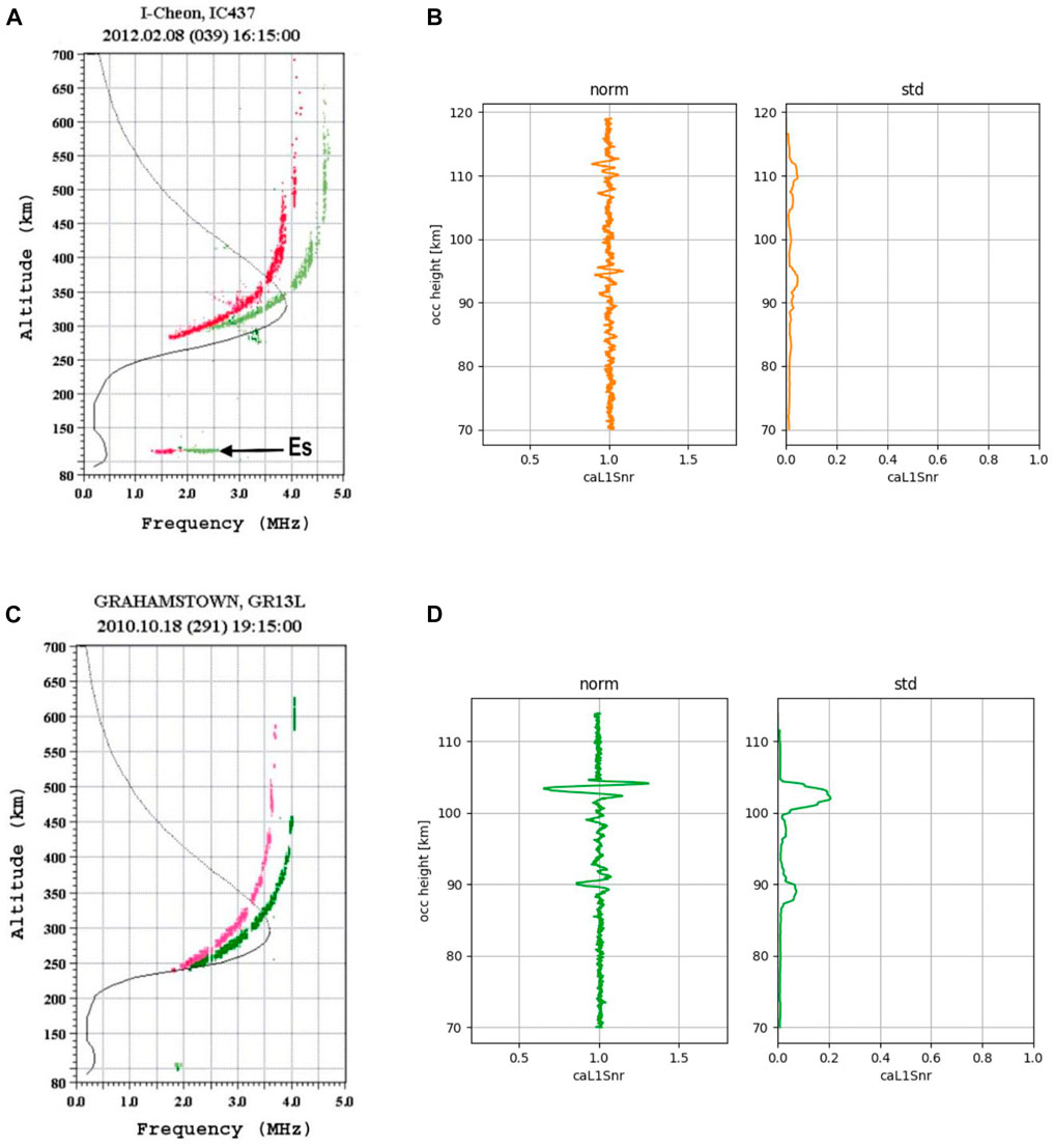
FIGURE 2. (A) Ionogram of the IC437 station (lat: 37.1° and lon: 127.5°) showing an Es layer on February 8, 2012, at 16:15. (B) SNR profile of a crossing radio occultation (lat: 37.3° and lon: 127.5°) showing no Es layer on February 8, 2012, at 16:12, and its corresponding standard deviation profile. (C) Ionogram of the GR13L station (lat: -33.3° and lon: 26.5°) showing no Es layer on October 18, 2010, at 19:15. (D) SNR profile of a crossing radio occultation (lat: -33.4° and lon: 26.6°) showing an Es layer on October 18, 2010, at 19:15, and its corresponding standard deviation profile.

The ionogram displays two distinct ionospheric echo traces, namely, the ordinary (pink) and extraordinary (green) traces, which are attributed to the ionosphere’s doubly refracting nature caused by the Earth’s magnetic field (FengJuan et al., 2022).

As an illustrative example of Type 3, we present Figure 2C, which showcases an ionogram obtained from the Grahamstown ionosonde station on October 18th, 2010, at 19:15. Upon examining the ionogram, it is evident that there is no recording of the ordinary mode Es layer. This absence of a distinct Es layer signature indicates that the concentration of plasma in the E layer is insufficient to meet the criteria for classification as an Es layer in the ionogram. This observation suggests that the conditions necessary for the formation of a well-defined Es layer were not present during the time of the recording at the Grahamstown station. In contrast, Figure 2D provides further insights by presenting the GPS L1 signal data collected from a location situated approximately 0.1° in latitude and longitude from the ionosonde station, at the same time as the ionogram recording. Notably, the GPS signal data reveal distinct disturbances in the altitude range of 100–110 km. These disturbances are indicated by a standard deviation greater than 0.2, exceeding our predetermined criteria for detecting an Es layer in radio occultation data. Therefore, based on our criteria, we can confidently confirm the detection of an Es layer using the radio occultation technique.

In order to better understand the discrepancy between ground-based and satellite technique in Es layer detection, we performed a statistical analysis using a multi-year dataset of crossing observations at six stations. The analysis has been performed within different distances from the center station, at different seasons, and local times. The subsequent sections present statistical results of conjunctions at the Pruhonice station (50° N and 14.6ºE) as an example of two separate cases: case 1 refers to conjunction data points in which an Es layer is detected through the radio occultation technique and is either confirmed by ionograms or not (Es_{radio-occultation} = 1); case 2 is characterized by the detection of an Es layer through ionograms while radio occultation signals may or may not be affected by the Es layer (Es_ionogram = 1). It is important to note that in all the following results, the agreement rate between the two methods in case 1 is always higher than in case 2. This can be simply explained by results in the confusion matrix presented in Table 2. The number of conjunction observations in which the Es layer is detected by an ionogram and not by radio occultation is almost half of those in the reverse type.

3.1 Local dependence of the ground/satellite Es agreement

The conjunction observations were classified into 0.5° latitude bands based on their distance from the Pruhonice station. The agreement between Es events derived from the ionosonde and radio occultation was then measured and presented in Table 3 for both cases. In case 1, each latitude band contained approximately 220 conjunction observations, while in case 2, there were approximately 330 observations in each latitude band. Similarly, the longitudinal dependence of the agreement between the two methods was examined in 1° longitude bands and presented in Table 4. For case 1, there were approximately 170 conjunction observations in each longitude band, while for case 2, there were approximately 260 observations.

TABLE 3

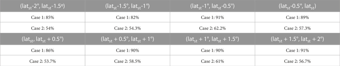
TABLE 3. Latitudinal dependence of the agreement between ionosonde and radio occultation measurements in detecting the Es layer (lat_st: latitude of the Pruhonice station). Case 1 represents Es _{radio-occultation} = 1, while case 2 is Es_ionogram = 1.

TABLE 4

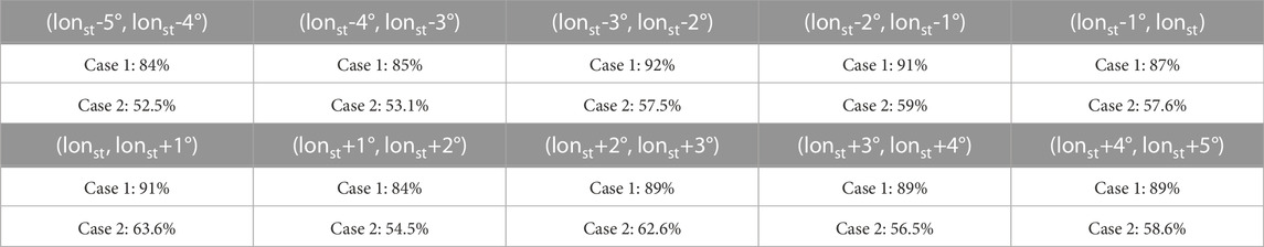
TABLE 4. Longitudinal dependence of the agreement between ionosonde and radio occultation measurements in detecting the Es layer (lon_st: longitude of the Pruhonice station). Case 1 represents Es _{radio-occultation} = 1, while case 2 is Es_ionogram = 1.

The agreement between the ionosonde and radio occultation measurements of Es recordings was examined at various latitudinal and longitudinal distances from the base station. The results revealed that there is no significant dependence on the distance from the ionosonde station in both cases. This implies that the discrepancy in Es detection between ground-based and satellite techniques is hardly influenced by the distance from the ionosonde station, provided that a 2° latitude × 5° longitude grid around each ionosonde is considered.

As presented in Table 5, the altitude dependence of the agreement between ionogram and radio occultation observation in detecting Es layers was studied in 5 km altitude bands. In both cases, the agreement between the two methods increased with the increase in altitude and reached its maximum at 105–115 km. However, beyond this height range, the agreement dropped. This trend is because the maximum amplitude of Es occurrence is found at heights between 95 and 115 km.

TABLE 5

TABLE 5. Altitude dependence of the agreement between ionosonde and radio occultation measurements in detecting the Es layer. Case 1 represents Es _{radio-occultation} = 1, while case 2 is Es_ionogram = 1.

3.2 Temporal dependence of the ground/satellite Es agreement

To proceed, the conjunction data were sorted into various seasons and local times to investigate if the agreement in detecting Es through two methods varies with the local time and season. Table 6 presents that in case 1, the highest level of agreement was observed in the local summer, whereas the lowest was seen in local winter. However, in case 2, the agreement demonstrated almost no dependence on the season. The number of conjunction data points is rather equally distributed during different months, in each station. For case 1, there were at least 230 conjunction observations in each longitude band, while for case 2, the minimum number of conjunction observations was approximately 380. Additionally, the results in Table 7 indicate that for case 1, the agreement was highest during the daytime and remained at a nearly consistent level during different local times for case 2. The number of conjunction observations studied at each local time grid was at least 100.

TABLE 6

TABLE 6. Seasonal dependence of the agreement between ionosonde and radio occultation measurements in detecting the Es layer. Case 1 represents Es _{radio-occultation} = 1, while case 2 is Es_ionogram = 1.

TABLE 7

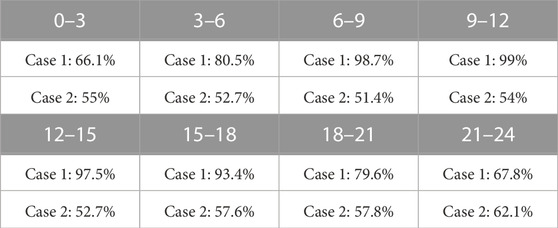
TABLE 7. Local time dependence of the agreement between ionosonde and radio occultation measurements in detecting the Es layer. Case 1 represents Es _{radio-occultation} = 1, while case 2 is Es_ionogram = 1.

The solar zenith angle dependence of the agreement between the ionosonde and radio occultation presented in Table 8 confirms our previous results.

TABLE 8

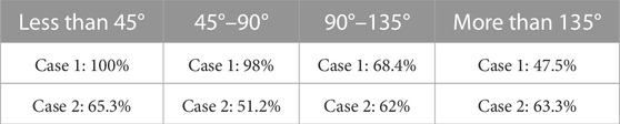
TABLE 8. Solar zenith angle dependence of the agreement between ionosonde and radio occultation measurements in detecting the Es layer. Case 1 represents Es _{radio-occultation} = 1, while case 2 is Es_ionogram = 1.

According to the seasonal and local time dependence of the Es detection agreement between the two methods, we can conclude that in case of observing a radio occultation signal disturbance that meets the criteria of Es layer detection proposed by Arras & Wickert (2018), there is a higher likelihood of recording an ionogram Es layer echo in a nearby location during the daytime and local summer.

All stations show similar spatial, seasonal, and local-time dependence. An overview of the monthly dependence of the Es detection via two different methods in case 1 is demonstrated in Figure 3A. The month-to-month agreement of the Es detection between the ionosonde and radio occultation in Pruhonice, I-Cheon, and Ramey of the Northern Hemisphere station is maximum during May, June, July, and August; on the other hand, the maximum in Grahamstown, Madimbo, and Learmonth in the Southern Hemisphere occurs during November, December, January, and February. As shown in Figure 3A, Learmonth on the right panel shows a better agreement with radio occultation observations in recording Es occurrences. This can be due to different technical aspects or operating software being used at different ionosonde stations.

FIGURE 3

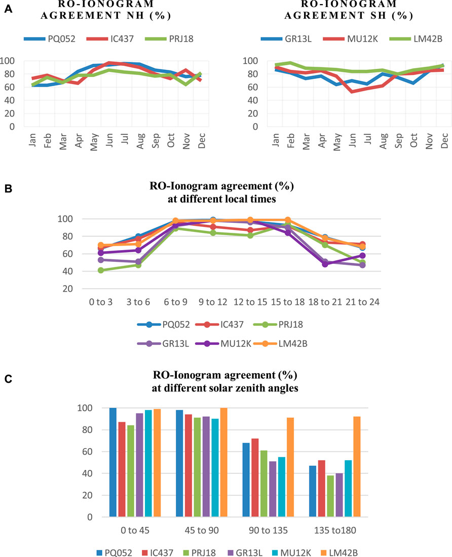
FIGURE 3. (A) Monthly dependence of the Es layer detection agreement when using radio occultation versus using ionosonde at the Northern Hemisphere (left) and Southern Hemisphere (right). (B) Local time dependence of the Es layer detection agreement when using radio occultation versus using ionosonde. (C) Solar zenith angle dependence of the Es layer detection agreement when using radio occultation versus using ionosonde. These results are related to case 1 (Es_{radio-occultation} = 1).

According to the results presented in Figure 3B, Es layers recorded in the ionogram agree largely with those in radio occultation measurements during local times between 6 and 18. During this time period, the agreement is greater than 80% in all stations. However, during night time, it can go down to 40% at some stations. Supporting that, as shown in Figure 3C, all ionosonde Es layer recordings have a greater agreement with Es layers detected in satellite observations when the solar zenith angle is less than 90°.

We conducted a similar study on other stations to examine the temporal dependence of the agreement between the two methods for case 2 in which all conjunction ionograms record an Es layer. However, no specific daily, monthly, or local dependence was discovered. Additionally, we analyzed the agreement year by year for each station to assess the influence of the 11-year solar cycle. The findings revealed that the agreement between the two methods remained relatively constant, with no significant differences indicating no solar cycle dependence.

3.3 Es intensity dependence of the ground/satellite Es agreement

We examined the dependence of the agreement between the two Es detection methods on the intensity of the Es layer by looking into the S4 index in case 1 and foEs and fbEs parameters in case 2. The agreement between Es events measured by the radio occultation technique with the Es layers recorded in the ionogram has been measured in 0.2 length S4 bands and presented in Table 9. As shown in the table, the agreement increases with the increase in S4. Therefore, the higher the Es intensity detected by the satellite is, the more probable it is to observe an Es layer in the conjunction ionogram.

TABLE 9

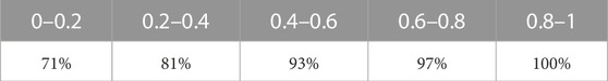
TABLE 9. S4 dependence of the agreement between ionosonde and radio occultation measurements in detecting the Es layer at IC437.

In order to examine the Es intensity dependence in case 2, we studied the foEs dependence of the satellite and ground-based Es detection agreement. The results are presented in Table 10. In general, the agreement increases as the foEs becomes larger, but the agreement rate drops as foEs goes higher than 4.5–5 MHz.

TABLE 10

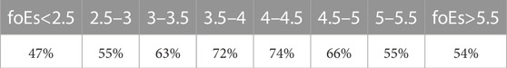
TABLE 10. foEs dependence of the agreement between ionosonde and radio occultation measurements in detecting the Es layer at IC437.

Based on our analysis, more than 80% (i.e., 3798 blanketing Es events of the 9,000 conjunction points presented in Table 2) of the Es events in mid- and low-latitude regions were found to be blanketing Es. By taking into account only the blanketing-type Es and repeating all previous analyses, the temporal and spatial dependence of the Es detection method agreement stays the same. Therefore, we conducted an analysis to study the fbEs dependence of the ionosonde and satellite method agreement in detecting Es layers. The fbEs results presented in Table 11 were similar to the foEs.

TABLE 11

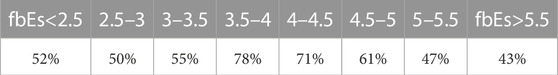
TABLE 11. fbEs dependence of the agreement between ionosonde and radio occultation measurements in detecting the Es layer at IC437.

4 Discussion

According to Table 10, when the foEs value is greater than average, the agreement between the two methods in detecting the Es layer decreases. We also noticed that 64.4% of these conjunction observations with a high fbEs value had an extremely large SNR value as well. Figure 4 provides two examples of such events. Figure 4A shows a strong blanketing Es, and in Figure 4B, there is a crossing radio occultation signal which is highly disturbed but not marked as an Es event. Arras and Wickert (2018) only showed tag signals with a standard deviation greater than 0.2 within the altitude range of 10 km as an Es layer. By applying these criteria, very strong Es layers, which cause very big standard deviation at a high-altitude band, will sometimes be overlooked.

FIGURE 4

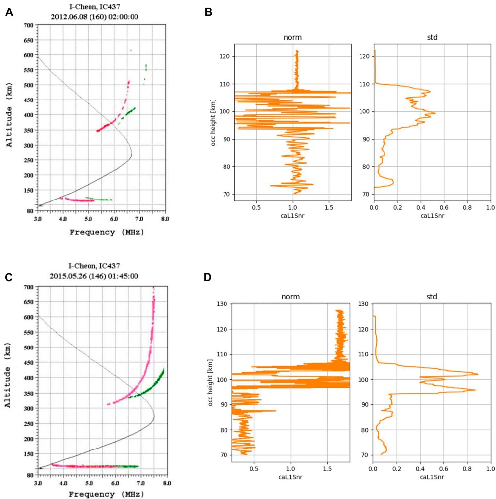
FIGURE 4. (A) Ionogram of the IC437 station (lat: 37.1° and lon: 127.5°), June 8, 2012, 2:00. (B) SNR profile of a crossing radio occultation (lat: 36.9° and lon: 130.7°) on June 8, 2012, at 1:55, and its corresponding standard deviation profile. (C) Ionogram of the IC437 station (lat: 37.1° and lon: 127.5°), May 26, 2015, 1:45. (D) SNR profile of a crossing radio occultation (lat: 36.9° and lon: 129.6°) on May 26, 2015, at 1:48, and its corresponding standard deviation profile.

Figure 4C is another example of a severe Es layer that blankets the echo from upper layers of ionosphere. As shown in Figure 4D, the radio occultation signal traveling from above reaches an Es layer at approximately 110 km and gets disturbed intensely. As a result of this disturbance, the normalized SNR reduces to less than one third of its initial amount. Such severe disruptions (in this case foEs = 6.3 MHz) caused by Es events can sometimes result in GNSS signal loss (Yue et al., 2016). Hence, despite the global Es data coverage that radio occultation provides, it seems that further improvements can be applied to the Es detection criteria proposed by Arras and Wickert (2018).

The discrepancy between Es layers detected in ionograms and those observed in radio occultation might also exist due to limitations in the Es layer detection capability of the ground-based techniques. The ionosonde data used in this study are all derived from the Lowell data center. Nevertheless, it should be noted that the stations do not always utilize the same software. Furthermore, there are variations in hardware and technical aspects across different stations, including variations in antenna configurations from site to site. Factors such as sounding frequency, antenna type, system maintenance, and other technical considerations can potentially influence the detectability of Es layers. As demonstrated in Figures 3A, D, although the Learmonth station follows the same temporal dependence as other Southern Hemisphere stations, it has always a higher agreement rate with radio occultation observations in comparison to others. Ionosonde stations have different limits of density sensitivity, depending on their operating mode. Therefore, the detectability of the Es layer can depend on the ionosonde station and vary from one ionosonde to another based on their different software and technical facilities. Additionally, it is always possible to have human errors, when scaling ionograms manually.

Another potential factor contributing to the observed discrepancies between ground-based and satellite measurements of Es layers is the fundamental difference in the Es detection mechanisms employed by the two methods. It is important to recognize that ionosonde and satellite observations utilize distinct approaches to detect Es layers, which can yield divergent measurements of these atmospheric phenomena. These inherent dissimilarities in detection mechanisms may offer a plausible explanation for the contradictory findings observed between ground-based and satellite techniques. In ionosonde observations, Es layers are typically identified and recorded in ionograms by analyzing the electron density of the E layer, which is derived from the transmitted ionosonde signal. The ionogram provides information about the plasma density distribution within the ionosphere, allowing for the detection of Es layers based on their characteristic electron density patterns. However, in the radio occultation technique employed by satellites, the detection of Es layers relies on the observation of electron density gradients that induce scintillations in the global navigation satellite system (GNSS) signals. In this case, it is the presence and magnitude of these gradients that are indicative of the presence of Es layers. This fundamental disparity in the underlying mechanisms for Es detection between ground-based ionosondes and satellite-based radio occultation techniques can give rise to varying measurements of Es layers obtained through each method. For instance, there may be cases where an Es layer, such as the one depicted in Figure 2C, exhibits a plasma density that is too weak to be discerned and recorded in an ionogram. However, despite the lower plasma density, the associated electron density gradient can still be significant enough to cause disturbances in radio occultation signals, leading to their detection using satellite observations. This physical distinction in the detection approaches of the two methods may also provide an explanation for the observed maximum agreement between ground-based and satellite techniques during the daytime and local summer periods, as these conditions can favor the generation of notable electron density gradients within the Es layer.

5 Conclusion

In this study, we conducted a comprehensive comparison between the Es recordings obtained from six mid- and low-latitude ionosonde stations and the corresponding FORMOSAT-3/COSMIC radio occultation measurements, utilizing the method proposed by Arras & Wickert (2018). Our analysis focused on examining the local and temporal variations in the agreement between the ground-based and satellite techniques for detecting Es layers. The key findings of our investigation are summarized as follows:

1. At different ionosonde stations, we observed a noticeable disagreement of 20%–40% between the ground-based and satellite measurements of Es layer occurrence. The extent of this discrepancy varied depending on factors such as local time, season, and altitude at which an Es event occurred. These findings emphasize the importance of considering the specific conditions under which Es layers are detected.

2. Our results indicate that the agreement between ground-based and satellite measurements of Es layer occurrence is highest during local summer and daytime. When the Es detection method proposed by Arras & Wickert (2018) identifies an Es layer in radio occultation observations, it tends to align more closely with the ground-based measurements during these specific periods.

3. We observed that certain ionosonde stations demonstrated a consistently stronger agreement with satellite Es observations throughout the year. This observation suggests that differences in technical facilities and measurement software among ionosonde stations may influence their compatibility in Es detection. Further investigation into these variations can provide valuable insights into improving the overall consistency between ground-based and satellite techniques.

4. The detection capability of Es layers using radio occultation data is dependent on the specific criteria employed in the analysis of GNSS signals. For instance, our study identified instances where severe Es layers were not captured in the radio occultation data due to their high signal standard deviation across a wide range of altitudes. This observation underscores the need for careful consideration and refinement of the criteria used in analyzing GNSS signals to enhance the detection and characterization of Es layers.

5. A fundamental distinction exists between ground-based ionograms and satellite techniques in measuring Es layers. Ionograms record the E region plasma density, while satellite techniques focus on measuring the E region plasma density gradient, responsible for GNSS signal scintillations. This inherent difference contributes to observed discrepancies. Additionally, it explains the higher agreement during daytime and summer, characterized by more pronounced plasma density gradients. This information highlights that there is no single definition of Es layers that can simultaneously satisfy both satellite and ground-based observations. In future studies, it is helpful to clearly define Es for each investigation and be mindful of the disparities between the chosen approaches.

In conclusion, our study conducts a comparison of ground-based and satellite measurements of Es layers, shedding light on the local and temporal factors influencing their agreement. While acknowledging the limitations and specific conditions of our study, further investigations can build upon these findings to refine the detection and characterization of Es layers and enhance the overall understanding of ionospheric dynamics. Future research should explore alternative data analysis techniques, incorporate a larger number of ionosonde stations, and consider additional factors that may impact the agreement between ground-based and satellite measurements. By addressing these aspects, we can advance our knowledge of Es layers and their impact on ionospheric behavior in different regions and seasons.

Data availability statement

Publicly available datasets were analyzed in this study. These data can be found at: The level 1b atmPhs radio occultation data from the F3/C mission are available at the COSMIC Data Analysis and Archive Center: https://www.cosmic.ucar.edu/what-we-do/cosmic-1/data/. Ionosonde recordings are available at GIRO: https://giro.uml.edu/didbase/.

Author contributions

SS-M performed the data analysis and wrote the paper. YY discussed the results and contributed to revise the paper. CA extracted the Es events from the SNR of the RO signal. DT provided guidance on ionogram scaling and supported the interpretation of the ionograms. All authors contributed to the article and approved the submitted version.

Funding

This study received partial support from JSPS and DFG (Grant YA-574-3-1) through the Joint Research Projects LEAD with DFG (JRPs-LEAD with DFG). Additionally, it was partly funded through the “Open-Access-Publikationskosten” program by DFG, Project Number 491075472.

Acknowledgments

SS-M would like to express gratitude to Dr. Veronika Barta for providing valuable insights on the interpretation of ground-based observations. CA acknowledges the support by Deutsche Forschungsgemeinschaft (DFG) under grant WI 2634/19-1.

Conflict of interest

The authors declare that the research was conducted in the absence of any commercial or financial relationships that could be construed as a potential conflict of interest.

Publisher’s note

All claims expressed in this article are solely those of the authors and do not necessarily represent those of their affiliated organizations, or those of the publisher, the editors, and the reviewers. Any product that may be evaluated in this article, or claim that may be made by its manufacturer, is not guaranteed or endorsed by the publisher.

References

Arras, C. (2010). A global survey of sporadic E layers based on GPS Radio occultations by CHAMP, GRACE and FORMOSAT–3/COSMIC, Deutsches GeoForschungsZentrum GFZ Potsdam].

Google Scholar

Arras, C., Jacobi, C., Wickert, J., Heise, S., and Schmidt, T. (2010). Sporadic E signatures revealed from multi-satellite radio occultation measurements. Adv. Radio Sci. 8, 225–230. doi:10.5194/ars-8-225-2010

CrossRef Full Text | Google Scholar

Arras, C., Resende, L. C. A., Kepkar, A., Senevirathna, G., and Wickert, J. (2022). Sporadic E layer characteristics at equatorial latitudes as observed by GNSS radio occultation measurements. Earth, Planets Space 74 (1), 163–215. doi:10.1186/s40623-022-01718-y

CrossRef Full Text | Google Scholar

Arras, C., Wickert, J., Beyerle, G., Heise, S., Schmidt, T., and Jacobi, C. (2008). A global climatology of ionospheric irregularities derived from GPS radio occultation. Geophys. Res. Lett. 35 (14), L14809. doi:10.1029/2008gl034158

CrossRef Full Text | Google Scholar

Arras, C., and Wickert, J. (2018). Estimation of ionospheric sporadic E intensities from GPS radio occultation measurements. J. Atmos. Solar-Terrestrial Phys. 171, 60–63. doi:10.1016/j.jastp.2017.08.006

CrossRef Full Text | Google Scholar

Axford, W., and Cunnold, D. (1966). The wind-shear theory of temperate zone sporadic E. Radio Sci. 1 (2), 191–197. doi:10.1002/rds196612191

CrossRef Full Text | Google Scholar

Baggaley, W. (1984). Ionospheric sporadic-E parameters: Long-term trends. Science 225 (4664), 830–833. doi:10.1126/science.225.4664.830

PubMed Abstract | CrossRef Full Text | Google Scholar

Carmona, R. A., Nava, O. A., Dao, E. V., and Emmons, D. J. (2022). A comparison of sporadic-E occurrence rates using GPS radio occultation and ionosonde measurements. Remote Sens. 14 (3), 581. doi:10.3390/rs14030581

CrossRef Full Text | Google Scholar

Chandra, H., and Rastogi, R. (1975). Blanketing sporadic E layer near the magnetic equator. J. Geophys. Res. 80 (1), 149–153. doi:10.1029/ja080i001p00149

CrossRef Full Text | Google Scholar

Christakis, N., Haldoupis, C., Zhou, Q., and Meek, C. (2009). Seasonal variability and descent of mid-latitude sporadic E layers at Arecibo. Ann. Geophys. 27 (3), 923–931. doi:10.5194/angeo-27-923-2009

CrossRef Full Text | Google Scholar

Chu, Y.-H., Wang, C., Wu, K., Chen, K., Tzeng, K., Su, C.-L., et al. (2014). Morphology of sporadic E layer retrieved from COSMIC GPS radio occultation measurements: Wind shear theory examination. J. Geophys. Res. Space Phys. 119 (3), 2117–2136. doi:10.1002/2013ja019437

CrossRef Full Text | Google Scholar

FengJuan, S., XianRong, W., HongBo, Z., Bao, Z., PanPan, B., and Hongyan, C. (2022). Statistical and simulation study on the separation in junction frequencies between ordinary (O) and extraordinary (X) wave in oblique ionograms. Earth, Planets Space 74 (1), 189–214. doi:10.1186/s40623-022-01755-7

CrossRef Full Text | Google Scholar

Gan, C., Hu, J., Luo, X., Xiong, C., and Gu, S. (2022). Sounding of sporadic E layers from China Seismo-Electromagnetic Satellite (CSES) radio occultation and comparing with ionosonde measurements. Ann. Geophys. 40 (4), 463–474. doi:10.5194/angeo-40-463-2022

CrossRef Full Text | Google Scholar

Gooch, J. Y., Colman, J. J., Nava, O. A., and Emmons, D. J. (2020). Global ionosonde and GPS radio occultation sporadic-E intensity and height comparison. J. Atmos. Solar-Terrestrial Phys. 199, 105200. doi:10.1016/j.jastp.2020.105200

CrossRef Full Text | Google Scholar

Haldoupis, C. (2011). “A tutorial review on sporadic E layers,” in Aeronomy of the Earth's atmosphere and ionosphere (Springer), 381–394.

CrossRef Full Text | Google Scholar

Haldoupis, C. (2012). Midlatitude sporadic E. A typical paradigm of atmosphere-ionosphere coupling. Space Sci. Rev. 168 (1), 441–461. doi:10.1007/s11214-011-9786-8

CrossRef Full Text | Google Scholar

Haldoupis, C., and Pancheva, D. (2002). Planetary waves and midlatitude sporadic E layers: Strong experimental evidence for a close relationship. J. Geophys. Res. Space Phys., 107 (A6), 3–6. doi:10.1029/2001JA000212

CrossRef Full Text | Google Scholar

Haldoupis, C., Pancheva, D., Singer, W., Meek, C., and MacDougall, J. (2007). An explanation for the seasonal dependence of midlatitude sporadic E layers. J. Geophys. Res. Space Phys. 112 (A6). doi:10.1029/2007ja012322

CrossRef Full Text | Google Scholar

Harris, R., and Taur, R. (1972). Influence of the tidal wind system on the frequency of sporadic-E occurrence. Radio Sci. 7 (3), 405–410. doi:10.1029/rs007i003p00405

CrossRef Full Text | Google Scholar

Igarashi, K., Nakamura, M., Wilkinson, P., Wu, J., Pavelyev, A., Wickert, J., et al. (2001). Global sounding of sporadic E layers by the GPS/MET radio occultation experiment. J. Atmos. Solar-Terrestrial Phys. 63 (18), 1973–1980. doi:10.1016/s1364-6826(01)00063-3

CrossRef Full Text | Google Scholar

Leighton, H., Shapley, A., and Smith, E. (1962). International series of monographs on electromagnetic waves. Elsevier, 166–177.The occurrence of sporadic E during the IGY.

CrossRef Full Text | Google Scholar

Luo, J., Liu, H., and Xu, X. (2021). Sporadic E morphology based on COSMIC radio occultation data and its relationship with wind shear theory. Earth, Planets Space 73 (1), 212–217. doi:10.1186/s40623-021-01550-w

CrossRef Full Text | Google Scholar

MacDougall, J. (1978). Seasonal variation of semidiurnal winds in the dynamo region. Planet. space Sci. 26 (8), 705–714. doi:10.1016/0032-0633(78)90001-6

CrossRef Full Text | Google Scholar

Macleod, M. A. (1966). Sporadic E theory. I. Collision-geomagnetic equilibrium. J. Atmos. Sci. 23 (1), 96–109. doi:10.1175/1520-0469(1966)023<0096:seticg>2.0.co;2

CrossRef Full Text | Google Scholar

Mathews, J. (1998). Sporadic E: Current views and recent progress. J. Atmos. Solar-Terrestrial Phys. 60 (4), 413–435. doi:10.1016/s1364-6826(97)00043-6

CrossRef Full Text | Google Scholar

Matsushita, S. (1962). “Lunar tidal variations of sporadic E,” in Ionospheric sporadic (Elsevier), 194–214.

CrossRef Full Text | Google Scholar

Merriman, D. K., Nava, O. A., Dao, E. V., and Emmons, D. J. (2021). Comparison of seasonal foEs and fbEs occurrence rates derived from global Digisonde measurements. Atmosphere 12 (12), 1558. doi:10.3390/atmos12121558

CrossRef Full Text | Google Scholar

Piggott, W. (1972). Handbook of Ionogram interpretation and reduction. US Department of Commerce.

Google Scholar

Qiu, L., Zuo, X., Yu, T., Sun, Y., and Qi, Y. (2019). Comparison of global morphologies of vertical ion convergence and sporadic E occurrence rate. Adv. Space Res. 63 (11), 3606–3611. doi:10.1016/j.asr.2019.02.024

CrossRef Full Text | Google Scholar

Reddy, C., and Matsushita, S. (1969). Time and latitude variations of blanketing sporadic E of different intensities. J. Geophys. Res. 74 (3), 824–843. doi:10.1029/ja074i003p00824

CrossRef Full Text | Google Scholar

Saksena, R. (1976). Possible effect of small and large wind shears on temperate latitude sporadic E. Indian J. Radio and Space Phys. 5, 235–239.

Google Scholar

Shinagawa, H., Miyoshi, Y., Jin, H., and Fujiwara, H. (2017). Global distribution of neutral wind shear associated with sporadic E layers derived from GAIA. J. Geophys. Res. Space Phys. 122 (4), 4450–4465. doi:10.1002/2016ja023778

CrossRef Full Text | Google Scholar

Sobhkhiz-Miandehi, S., Yamazaki, Y., Arras, C., Miyoshi, Y., and Shinagawa, H. (2022). Comparison of the tidal signatures in sporadic E and vertical ion convergence rate, using FORMOSAT-3/COSMIC radio occultation observations and GAIA model. Earth, Planets Space 74 (1), 88–13. doi:10.1186/s40623-022-01637-y

CrossRef Full Text | Google Scholar

Taguchi, S. (1961). World maps of foEs. J. Radio Res. Laboratory 8 (38).

Google Scholar

Wakai, N., Ohyama, H., and Koizumi, T. (1987). Manual of ionogram scaling. Japan: Radio Research Laboratory, Ministry of Posts and Telecommunications.

Google Scholar

Whitehead, J. (1970). Production and prediction of sporadic E. Rev. Geophys. 8 (1), 65–144. doi:10.1029/rg008i001p00065

CrossRef Full Text | Google Scholar

Whitehead, J. (1989). Recent work on mid-latitude and equatorial sporadic-E. J. Atmos. Terr. Phys. 51 (5), 401–424. doi:10.1016/0021-9169(89)90122-0

CrossRef Full Text | Google Scholar

Whitehead, J. (1961). The formation of the sporadic-E layer in the temperate zones. J. Atmos. Terr. Phys. 20 (1), 49–58. doi:10.1016/0021-9169(61)90097-6

CrossRef Full Text | Google Scholar

Wickert, J., Pavelyev, A., Liou, Y., Schmidt, T., Reigber, C., Igarashi, K., et al. (2004). Amplitude variations in GPS signals as a possible indicator of ionospheric structures. Geophys. Res. Lett. 31 (24), L24801. doi:10.1029/2004gl020607

CrossRef Full Text | Google Scholar

Wu, D. L., Ao, C. O., Hajj, G. A., de La Torre Juarez, M., and Mannucci, A. J. (2005). Sporadic E morphology from GPS-CHAMP radio occultation. J. Geophys. Res. Space Phys. 110 (A1), A01306. doi:10.1029/2004ja010701

CrossRef Full Text | Google Scholar

Yamazaki, Y., Arras, C., Andoh, S., Miyoshi, Y., Shinagawa, H., Harding, B., et al. (2022). Examining the wind shear theory of sporadic E with ICON/MIGHTI winds and COSMIC-2 radio occultation data. Geophys. Res. Lett. 49 (1), e2021GL096202. doi:10.1029/2021gl096202

CrossRef Full Text | Google Scholar

Yu, B., Xue, X., Scott, C. J., Yue, X., and Dou, X. (2022). An empirical model of the ionospheric sporadic E layer based on GNSS radio occultation data. Space weather. 20 (8), e2022SW003113. doi:10.1029/2022sw003113

CrossRef Full Text | Google Scholar

Yu, B., Xue, X., Yue, X. a., Yang, C., Yu, C., Dou, X., et al. (2019). The global climatology of the intensity of the ionospheric sporadic E layer. Atmos. Chem. Phys. 19 (6), 4139–4151. doi:10.5194/acp-19-4139-2019

CrossRef Full Text | Google Scholar

Yue, X., Schreiner, W. S., Pedatella, N. M., and Kuo, Y. H. (2016). Characterizing GPS radio occultation loss of lock due to ionospheric weather. Space weather. 14 (4), 285–299. doi:10.1002/2015sw001340

CrossRef Full Text | Google Scholar