Multi-wavelength observations and modeling of a microflare: constraining non-thermal particle acceleration

1 Introduction

Flares result from the rapid release of large amounts of energy via the magnetic reconnection process in the solar corona (e.g., Benz, 2008; Shibata and Magara, 2011; Testa and Reale, 2022). Such energy release efficiently accelerates particles, heats ambient plasma and generates magnetohydrodynamic (MHD) waves (e.g., Fletcher et al., 2011). Solar flares are typically catalogued in terms of their soft X-ray energy flux as measured by the Geostationary Orbiting Environmental Satellites (GOES). For example, microflares in the GOES A- or B-class range emit ≈6 orders of magnitude less energy than the largest GOES X-class flares. An increasing amount of evidence seems to suggest that smaller microflare or even nanoflare (even fainter, as-yet unresolvable events predicted by Parker (1988)) size events found in the core of active regions are in many aspects scaled-down versions of large flares, e.g., characterized by high temperatures (up to $\sim 10$ MK, Reale et al., 2019a; Reale et al., 2019b; Glesener et al., 2020; Testa et al., 2020; Testa and Reale, 2020; Cooper et al., 2020), and particle acceleration (Hannah et al., 2008; Testa et al., 2014; Wright et al., 2017; Testa et al., 2020; Glesener et al., 2020; Cooper et al., 2021). In addition, small flares occur much more frequently, possibly contributing to coronal heating (Hudson, 1991; Hannah et al., 2008).

Observations in the hard X-ray (HXR) range are a primary tool for studying particle acceleration. HXRs are emitted mainly via bremsstrahlung, with higher HXRs dominated by non-thermal bremsstrahlung, providing important observational signatures of the accelerated electron spectrum. A statistical study of approximately 25,000 microflares was conducted using the Reuven Ramaty High-Energy Solar Spectroscopic Imager (RHESSI), utilizing indirect Fourier imaging techniques (Christe et al., 2008; Hannah et al., 2008). RHESSI was sensitive to energies between 3 keV and 17 MeV, but experienced lower sensitivity to faint events due to high background from large detector volume (Lin et al., 2002). The Nuclear Spectroscopic Telescope ARray (NuSTAR) instrument (Harrison et al., 2013) is an astrophysical-focused mission which utilizes direct-focusing HXR telescopes, capable of achieving greater sensitivity to fainter events. NuSTAR solar observations are performed rarely (a few times per year), usually consisting of a few to several hours for each observation. Previous NuSTAR studies include analysis of both GOES sub-A-class quiet Sun brightenings (Glesener et al., 2017) and GOES A-class flares from active regions (Wright et al., 2017; Hannah et al., 2019; Glesener et al., 2020; Cooper et al., 2021). NuSTAR’s enhanced sensitivity has notably shown evidence of accelerated electrons below 7 keV, previously indistinguishable by RHESSI (Glesener et al., 2020). However, NuSTAR observations of non-thermal microflares are still somewhat rare, with Duncan et al. (2021) only definitively labeling one of the eleven studied A-class flares as exhibiting non-thermal emission. In both RHESSI and NuSTAR microflare studies, steeper non-thermal spectra have often been observed as compared to larger solar flares, resulting in more difficulty distinguishing an accelerated electron spectrum from thermal emission. Such work can be complemented by a multi-wavelength approach to analysis, particularly by including the chromospheric response to such accelerated electrons.

Our understanding of both large and small flare events has greatly improved since the launch of the Interface Region Imaging Spectrograph (IRIS; De Pontieu et al., 2014) in 2013. We refer the readers to Sections 4.6 and 5 of De Pontieu et al. (2021) for a recent review of the most significant results from IRIS in these topics. For instance, IRIS observations of footpoint brightenings associated with coronal nano to microflares has provided unexpected new indirect diagnostics of the presence of non-thermal particles in small heating events (e.g., Testa et al., 2014). These small coronal heating events induce rapid variability in the lower atmospheric (transition region and chromosphere) emission (e.g., Testa et al., 2013), and early IRIS observations, combined with simulations, showed that their spectral properties are crucially dependent on the mechanism of energy transport (e.g., thermal conduction vs non-thermal particles), and duration of the heating. In particular, IRIS Si iv blueshifts and Mg ii triplet emission are signatures of non-thermal particles, and the IRIS spectral properties also provide valuable diagnostics of the properties of the non-thermal particles, such as the low-energy cutoff (E_C) of their power-law distributions and total energy (Testa et al., 2014; Polito et al., 2018; Testa et al., 2020; Cho et al., 2023). These new IRIS indirect diagnostics of accelerated particles in small events are particularly interesting because of their sensitivity to small events which are typically difficult to observe in HXRs, and because of their diagnostics of the non-thermal particles properties (especially E_C), which are often difficult to tightly constrain with HXR spectra because of the overlap of thermal and non-thermal spectra.

Joint analysis has previously been performed combining IRIS, RHESSI and modeling for large flares (e.g., Polito et al., 2016; Rubio da Costa et al., 2016), achieving a more detailed understanding of flare energy release processes. The only previously combined NuSTAR and IRIS analysis is presented in Hannah et al. (2019), which analyzed a microflare with a background-subtracted GOES class of A1. Non-thermal emission was not detected, but the ability to connect NuSTAR’s HXR detection of 5 MK flare-heated plasma to transition region and chromospheric signatures with IRIS provided evidence for the usefulness of joint analysis between the two instruments.

In this paper we analyze coordinated observations with IRIS and NuSTAR of a B-class flare, which provide a rare opportunity to study non-thermal particles in a small flare using two independent diagnostics. NuSTAR observations provide a direct measure of flare-accelerated electrons, while IRIS reveals, with great sensitivity, the chromospheric response to those electrons. Hydrodynamic modeling performed using the RADYN model connect these observables. As discussed above, the IRIS diagnostics are indirect diagnostics, based on the predictions of state-of-the-art RADYN modeling. The analysis presented here therefore serves as a validation of our previous interpretation of the IRIS observations based on hydrodynamic modeling.

The paper is organized as follows. In Section 2 we describe the SDO, IRIS and NuSTAR observations analyzed in this work. Sections 3 and 4 present the details of the IRIS and NuSTAR spectroscopic observations for the event under study, while Section 5 and 6 present the results of the hydrodynamic modeling and three-dimensional magnetic field extrapolation. Finally, in Section 7 we summarise and discuss our results.

2 Observations of the 29 April 2021 B-class flare

The small B-class flare under study was part of a series of B-class flares that occurred on 29 April 2021 in the active region (AR) complex 12820/12821 from around 14 UT and that culminated in a C-class flare around 22:30 UT. Some of these small flares were observed by a combination of instruments, including Hinode, IRIS and NuSTAR, as part of the coordinated IRIS–Hinode Operation Plan (IHOP) 409 “Energetics of solar eruptions from the chromosphere to the inner heliosphere”¹. Figure 1 shows the evolution of the energy flux for the flares as observed by the GOES satellite in soft X-rays. The light blue curve and blue, magenta, and green arrows highlight the time intervals of the NuSTAR, IRIS, Hinode/EIS and VLA observational coverage respectively. In this work we focus on studying the small flare around 18:20 UT, that was observed by both IRIS and NuSTAR. While NuSTAR also observed the previous B-class flare around 18 UT, which occurred in the same active region (see Sect. 2.3), as well as a larger flare around 20 UT, these two events were not observed under the IRIS spectrograph slit. Unfortunately, the 18:20 UT microflare was not observed by Hinode/EIS and VLA, so we do not focus on these instruments in this work.

FIGURE 1

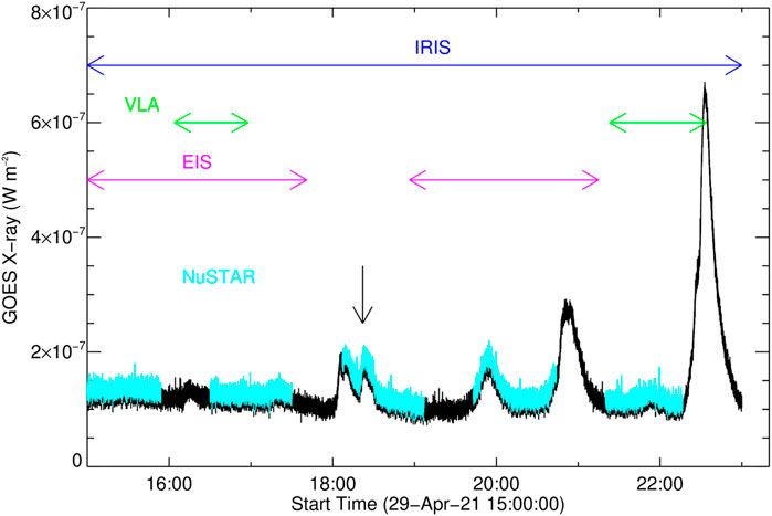
FIGURE 1. Overview of the 29 April 2021 flare observations and instrument coverage. The blue color indicates the NuSTAR observing time, and the horizontal arrows indicate the start and end time of the spectroscopic observations by IRIS and EIS, as well as VLA. The black vertical arrow indicates roughly the time of the microflare understudy. Unfortunately this flare was not observed by EIS and VLA.

Figure 2 shows an overview of the B-class flare under study as observed by the Atmospheric Imaging Assembly (AIA) 304 Å (panel a) and 94 Å (panel b) filters, showing plasma formed at around 7 ⋅ 10⁶ K (7 MK, respectively O’Dwyer et al., 2010; Martínez-Sykora et al., 2011; Boerner et al., 2012; Testa and Reale, 2012, see Sect. 2.1). The 94 Å images have been processed to isolate the contribution from the Fe xviii line, using an established linear combination of the flux observed in AIA’s 94, 171 and 211 Å channels (Del Zanna, 2013). An animation associated with Figure 2 shows the evolution of the plasma emission over time. The larger and smaller boxes overlaid on the AIA images indicate the field-of-view (FOV) of the IRIS Slit-Jaw Imager (SJI) and spectrograph respectively. Panel c) shows an image from the IRIS SJI C ii 1,330 Å filter, dominated by plasma formed at T ≈ 10–40 ⋅ 10³ K (10–40 kK). The bright structure visible in both the 304 Å and the IRIS SJI images is the mini-ribbon of the B flare, where we observe interesting spectral features in the IRIS data. We describe these features in detail in Section 2.2. The analysis of the NuSTAR hard X-ray observations is described in Section 2.3.

FIGURE 2

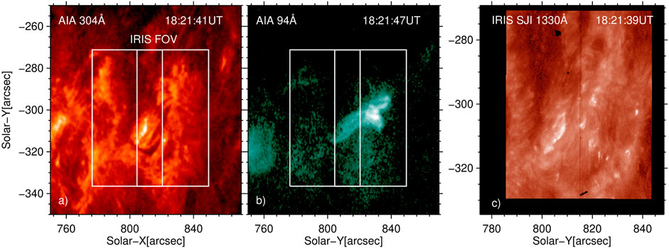
FIGURE 2. B-class flares around 18:20 UT as observed by the AIA 304 Å (Panel A), 94Å (Panel B) channels and the IRIS SJI 1330 Å (Panel C) channel. The IRIS FOV is also overlaid on the AIA images. An animation of this figure is available.

2.1 SDO observations

Extreme ultraviolet (EUV) context data from the Atmospheric Imaging Assembly (AIA; Lemen et al., 2012) on-board the Solar Dynamics Observatory spacecraft (Pesnell et al., 2012, SDO) is utilized as a large FOV context to our spectroscopic observations, for co-alignment between IRIS and NuSTAR observations, and to account for NuSTAR’s inherent pointing uncertainty when performing solar observations, as discussed in Section 2.3. The AIA 94 Å channel contains two temperature response peaks. The higher of the two is centered around 7 MK (e.g., O’Dwyer et al., 2010; Boerner et al., 2012; Testa and Reale, 2012), making it sensitive to temperatures measured by NuSTAR for flaring plasma. AIA 94 Å context images were made for the 18:20 UT flare, as well as the background time utilized in NuSTAR analysis. We isolate the higher temperature response peak in the 94 Å ∼channel due to Fe xviii∼via a linear combination of observed flux from AIA’s 94, 171, and 211 Å channels (Del Zanna, 2013). We have also used AIA 304 Å and 1600 Å images as context to our observations and to co-align the IRIS and AIA observations. Both filters show the cooler emission from the small ribbon that is also visible in the SJI images (see Figure 2).

We also analyze photospheric vector magnetograms and line-of-sight magnetic field intensities provided by the Helioseismic and Magnetic Imager (Scherrer et al., 2012, HMI) on board SDO. We use HMI data to derive a magnetic field extrapolation and obtain information about the magnetic connectivity of the flare loops under study (Sect. 6), which is useful to compare the results of the spectroscopic observations and models (Sect. 7). Both AIA images and HMI line-of-sight magnetic field intensity maps were processed and corrected for instrumental effects by using the standard SolarSoft routine aia_prep.pro.

2.2 IRIS observations

Since July 2013, IRIS has been providing far ultraviolet (FUV) and near ultraviolet (NUV) images and spectra of the solar atmosphere, from the photosphere to low corona, at very high spatial (0.33–0.4″), spectral (2.7 km s⁻¹ per pixel) and temporal resolution (down to 1s or less in high-cadence flare mode, De Pontieu et al., 2014). The IRIS spectrograph channel observes line and continua formed over a broad range of temperatures, from logT [K] ≈ 3.5–7. Simultaneously, the IRIS Slit-Jaw Imager (SJI) provides high-resolution (0.33″) context images in four individual filters (C ii 1330 Å, Si iv 1400 Å, Mg ii k 2796 Å and Mg ii h wing 2803 Å). Thanks to its unique instrumental capabilities, IRIS has significantly improved our understanding of the energy deposition in the lower atmosphere during flares (e.g., see De Pontieu et al., 2021, for a recent review).

The IRIS dataset under study was a part of a medium coarse 8-step raster observation, that ran between 13:59:21–22:58:59UT on 29 April 2021. A “coarse” raster means that there is a 2″ separation between consecutive IRIS slit positions. The medium raster FOV was ≈4′′× 60″, and the raster cadence was ≈75s, with an average raster step cadence of 8 s. IRIS SJI images in the 1330 Å filter were also taken with a cadence of 10 s over a ≈59′′× 60″ FOV. In this work, we use level 2 IRIS data, which have been corrected for a number of instrumental issues, including geometric, dark and flat-field calibration, and correction for the wavelength orbital variation (De Pontieu et al., 2014; Wülser et al., 2018).

2.3 NuSTAR observations

The Nuclear Spectroscopic Telescope ARray (NuSTAR), is a NASA small explorer mission launched in 2012. The instrument consists of two co-aligned direct-focusing HXR telescopes, with a 12′× 12′ FOV and angular resolution FWHM of 18′′ (Harrison et al., 2013). The identical CdZnTe solid-state focal plane detectors are made up of four pixel detector arrays (Madsen et al., 2015). Both detectors are used to improve sensitivity, and are defined as focal plane module A (FPMA) and focal plane module B (FPMB). NuSTAR is primarily an astrophysical observatory, with a total observation range of 3–79 keV. When used for solar observations, NuSTAR is limited to observing between 2.5–13 keV due to high count rates at low energies dominating the livetime during solar observations (Grefenstette et al., 2016). NuSTAR also experiences an uncertainty in absolute pointing of one to two arcmin when performing solar observations, which is accounted for by co-aligning NuSTAR data to AIA 94 Å images utilizing Sunpy’s calculate_match_template_shift function.

NuSTAR’s spatial data during this orbit is complex, with the active region producing two flares in different locations during a relatively short timescale. The first flare, occurring at 18:08 UT, is located at the eastern side of the active region. After this flare, the second flare occurs at 18:20 UT in the west, as shown in Figure 3. A background emission was measured at 18:40 UT after the second flare, with a background temperature of 4.4 MK found. Due to the quick succession of the flares, plasma heated above the background temperature is still present in the eastern region during the impulsive phase of the second flare. Because of this circumstance, we have carefully chosen source and background regions for spectroscopy, which will be further discussed in Sect. 4.2.

FIGURE 3

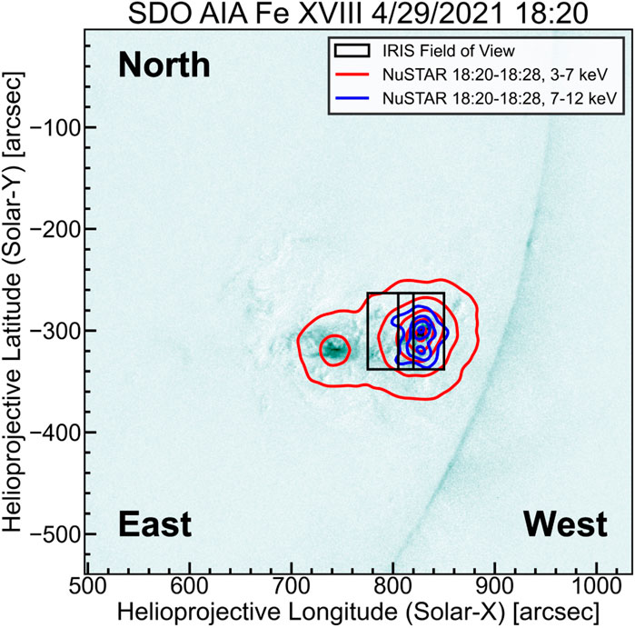
FIGURE 3. NuSTAR 25, 50, 75 and 95 percent contours of 3–7 keV (red) and 7–12 keV (blue) cross-correlated to AIA 94 Å to account for NuSTAR’s pointing uncertainty during solar observations. The IRIS FOV is shown in black, with the thin middle rectangle representing IRIS’s slit capable of spectroscopy. The western flare occurring at 18:20 UTC, shown on the right, is the primary subject of this study.

3 IRIS spectral observations in the small flare ribbon

We focus on the spectroscopic analysis of the small flare ribbon observed by IRIS under the slit in the Si iv (T ≈ 80 kK) line, formed in the transition region, as well as the C ii, Mg ii k and Mg ii triplet lines, formed at different heights across the chromosphere (Leenaarts et al., 2013a; b; Pereira et al., 2015).

Figure 4 shows an overview of the IRIS spectral observations during the B-class flare around 18:20 UT. Panels a) and f) show context images from the IRIS SJI 1330 Å (dominated by C ii emission) and AIA 94 Å filters respectively, with the IRIS raster FOV overlaid. The 94 Å images were processed to isolate the Fe xviii emission, as mentioned earlier in the text. A movie associated with Figure 4 and 6 shows the evolution of the emission and spectral parameters as a function of time. Panels b)–e) and g)–l) show the IRIS spectrograph data in the same FOV. In particular, panels b)–d) show the Si iv line intensity, Doppler shift velocity and full-width at half maximum (FWHM) as calculated by performing a single Gaussian fit image of the raster pixels, while panel e) shows the red-blue asymmetry (RB) of the Si iv line. The RB asymmetry describes the level of asymmetry of the line wings as compared to the peak and was calculated using the IDL routine gen_rb_profile_err.pro, available within the IRIS SolarSoft distribution and described by Tian et al. (2011). In this figure, we are showing the asymmetry calculated between ±30 km s⁻¹ from the line peak assuming a velocity interval of 5 km s⁻¹. In addition, panels g)–i) show the Mg ii k3 intensity, k2 peak difference and separation, respectively. The location of k3 and the k2 peaks for a typical Mg ii k reversed profile are shown in Figure 5G) for convenience. For the optically thick Mg ii line, Figure 4G) provides measurements of either the intensity of the reversed line core, when the line exhibits the typically central reverse profile (e.g., Figure 5G), or the peak intensity, when the line has a “single-peaked” type of profile (e.g., Figure 5C). The k2 peak difference and separation are calculated following formulas described in Polito et al. (2023), and they are ≈0 in case of single peaked type of profiles. Finally, panel l) shows the intensity of the Mg ii triplet line, calculated by integrating the intensity across the line profile between 2798.57 Å and 2799.1 Å, after subtracting a background taken between 2798 Å and 2798.3 Å (following Polito et al., 2023). Stronger intensities in panel l) (reversed color scale) indicate that the line is in emission, in contrast to a typical quiet Sun profile, where the lines would be mostly in absorption (Pereira et al., 2015).

FIGURE 4

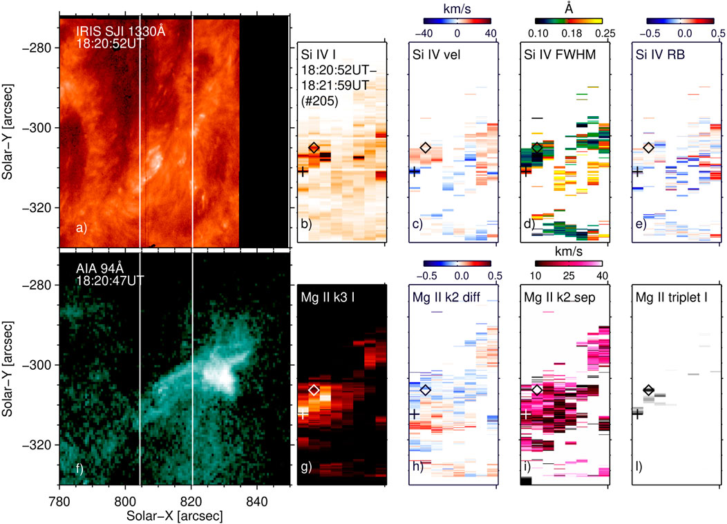
FIGURE 4. Observation of the B class flare around 18:20:50UT. Panel (A) IRIS SJI image in 1330 Å filter with the spectrograph FOV overlaid. Panels (B–E) IRIS spectroscopic observations in the Si iv line (intensity, Doppler shift velocity, FWHM and red-blue asymmetry. Panel (F) AIA 94 Å image with the IRIS spectrograph FOV overlaid. Panels (G–L) IRIS spectroscopic observations in the Mg ii line (intensity, k₂ peak difference and separation) and intensity of the Mg ii triplet line. The cross and diamond symbols in the IRIS spectroscopic rasters indicates a position where we observe respectively blueshifts and redshifts in the Si iv line in the mini-ribbon. An animation of this figure is available.

FIGURE 5

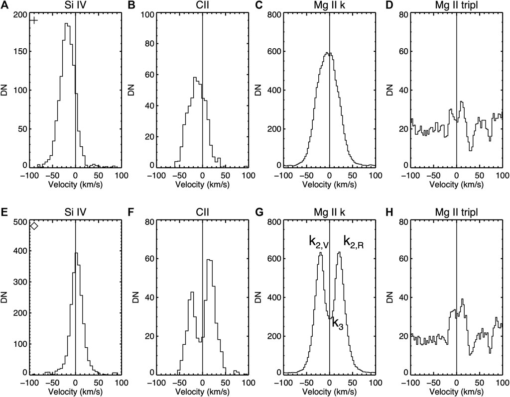
FIGURE 5. Spectra of IRIS lines : Si IV, CII, Mg II k and Mg II triplet in the location indicated by the cross (A–D) and diamond (E–H) in panels (B–E) and (G–L) of Figure 4.

Figure 4 shows that the Si iv line is either blue shifted or red shifted in the ribbons. The cross and diamond symbols in the IRIS rasters indicate pixels where we observe a Si iv blueshift (of the order of 20–30 km s⁻¹) and a gentle redshift (less than 5 km s⁻¹) respectively. The Si iv, C ii, Mg ii and Mg ii triplet spectra in these positions are shown in the top and bottom panels of Figure 5, respectively. In the same location as that of the Si iv blueshifted spectra we also see an increase in the FWHM and blue asymmetry of the line, as well as a decrease in the peak difference and separation of the Mg ii k line. A closer look to the spectra in Figure 5 reveals that the chromospheric lines in the locations of the Si iv blue shift within the small ribbon are characterized by a small line center reversal, with spectra that more closely resemble single peaked profiles, with no or small centroid Doppler shift for Mg ii (but a small blueshift for C ii), as well as an increased Mg ii triplet emission. For comparison, the spectra observed in the location indicated by the diamond symbol exhibit Mg ii and C ii chromospheric spectra with a stronger center reversal, but similarly enhanced Mg ii triplet emission. The variability in the behavior of these lines is consistent with the wide range of spectral features found in the statistical study of Testa et al. (2020) and the follow-up work by Cho et al. (2023), and with the predictions of RADYN simulations by Polito et al. (2018).

Figure 6 shows the same quantities as those of Figure 4 for the following IRIS raster (about 1 min later). The triangle symbol in this panel shows the location of a Si iv blue shift (also ≈25–30 km s⁻¹) that occurs in the same IRIS pixel as in the previous raster. The blue shift in this location is observed for 3 consecutive IRIS rasters, or about 4 min. This time period is significantly longer than for the events analyzed by Testa et al. (2020) who have presented statistical studies of IRIS brightenings in the ribbons for small nano or microflare events, and found Si iv brightenings with lifetime between 5 and 40s. However, for a significantly larger statistical sample ($\sim 1100$ events) of these small AR core heating events, Cho et al. (2023) find a somewhat uniform distribution of durations of Si iv brightenings up to 60 s, which was used as an upper limit of their selection criteria, therefore strongly suggesting a broad distribution of brightness duration for these events, and the presence of similar longer-lived events like the one studied here. Also, since the cadence of the raster in our observation is approximately 75 s, it is not clear whether the Si iv blueshift might have a shorter lifetime and simply appear and disappear in the same pixel within consecutive rasters as a consequence of recurring heating events in the same IRIS pixel (although possibly in separate field lines). The spectra shown in Figure 7 for the later blueshift indicated by the diamond symbol are relatively similar to those in Figure 5. Further, we note that the C ii line tends to be blueshifted (or with a blueshifted center reversal) in all 3 locations.

FIGURE 6

FIGURE 6. Observation of the B class flare around 18:22UT. For a description of the panels, see Figure 4. The triangle symbol in the IRIS spectroscopic rasters indicates a position where we observe blueshifts in the Si iv line in the mini-ribbon. An animation of this figure is available.

FIGURE 7

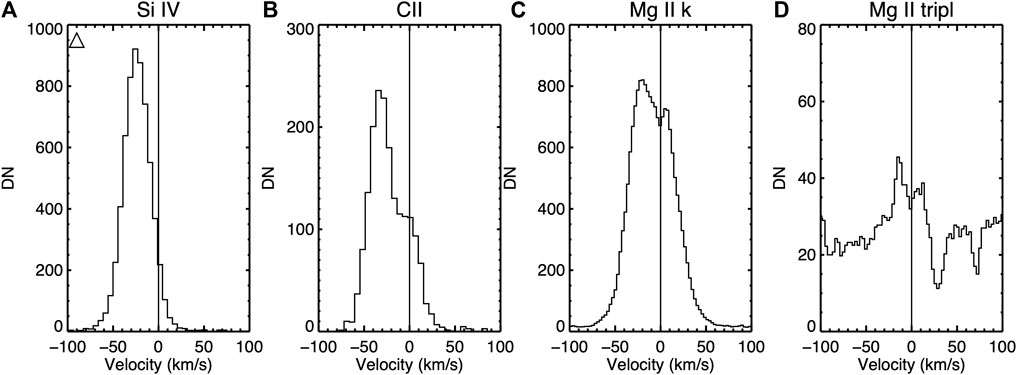
FIGURE 7. Spectra of IRIS lines : Si IV, CII, Mg II k and Mg II triplet in the location indicated by the triangle (A–D) in panels (B–E) and (G–L) of Figure 6.

As mentioned in Sect. 1, it has been shown that Si iv blueshifts and Mg ii triplet enhanced emission are crucial indirect signatures for the presence of non-thermal electrons (Testa et al., 2014; Polito et al., 2018; Testa et al., 2020). In this observation, for the first time in this type of study, we also have direct measurements of the accelerated electrons from NuSTAR, as described in the next Section.

4 Direct measurement of the accelerated electron distribution

In this section, we describe the spectral analysis of the NuSTAR data. Such analysis is crucial to confirm whether accelerated electrons are present in the small flare (as suggested by the IRIS spectral observations), and to provide measurements of the electron-beam distribution to guide the models (Sect. 5).

4.1 Temporal analysis

The lightcurves for this NuSTAR observation are shown in Figure 8. The middle two panels are livetime-corrected count rates for NuSTAR, separated into low and high energies. The top panel shows the total GOES short- and long-wavelength X-ray Sensor (XRS) SXR flux. The bottom panel includes both the high and low energy NuSTAR lightcurves, normalized to arbitrary units to best compare their time profiles. The derivatives of the NuSTAR 3–7 keV count rate and the long-wavelength GOES XRS flux, with a 2-min boxcar average to account for noise, are also included.

FIGURE 8

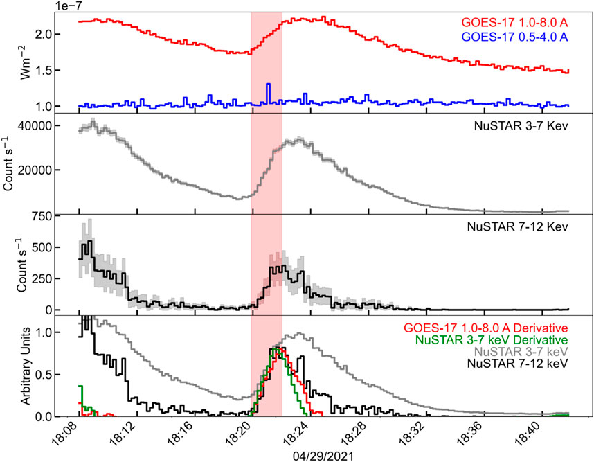
FIGURE 8. GOES and NuSTAR lightcurves, with the red shaded region representing the 2-min interval used for spectroscopy. Panel 1 shows the GOES XRS long and short-wavelength soft-xray flux. Panels 2 and 3 show the NuSTAR livetime-corrected lightcurves, separating the lower (3–7 keV) and higher (7–12 keV) energies. Panel 4 shows both NuSTAR lightcurves, and both the NuSTAR 3–7 keV and GOES 1.0–8.0 A derivatives (with 2-min boxcar averages) normalized to arbitrary units. The earlier peak of the higher energy NuSTAR lightcurve, with the NuSTAR low energy and GOES SXR derivatives matching that lightcurve, is indicative of the Neupert effect and suggests that the highest-energy NuSTAR emission is non-thermal.

The NuSTAR lightcurve displays noticeable similarities to those of larger flares and the standard flare model. The higher energy NuSTAR lightcurve shows an earlier peak time and greater impulsivity than the lower energy range. The change in lightcurve profile is at ∼7keV, which matches well to the found cutoff energies for accelerated electrons in spectral fitting (discussed in Section 4.2). Notably, the NuSTAR low energy and GOES SXR derivatives match the profile of the higher energy HXR lightcurve, exhibiting the Neupert effect (Neupert, 1968). The Neupert effect is often used to address the potential for non-thermal signatures. The derivative of SXR or EUV emission matching that of the higher energy HXRs suggests that thermal emission results from heating by accelerated electron beams (Neupert, 1968; Veronig et al., 2002; Dennis et al., 2003).

4.2 Spectral analysis

Spectroscopy of the 18:20 UT flare was performed using the X-ray spectral fitting package OSPEX and was independently confirmed using the package XSPEC. A 2-min window during the impulsive phase of the flare, highlighted in red in Figure 8, was used for spectral fitting. This early-flare phase was used in order to best search for signatures of accelerated electrons.

Solar observations result in significantly higher count rates than those experienced by NuSTAR when observing its astrophysical targets. Therefore, the detectors must be checked for pileup (discussed in Grefenstette et al., 2016; Appendix C). Detector pileup may occur when multiple photons enter a single pixel within a single measurement time, but are only recorded as a single event Harrison et al. (2013). NuSTAR events track the pattern of pixels in which charge was measured, or “grade.” Pulse pileup conditions may be checked by looking at the event rate of “unphysical grades”—combinations that are impossible to achieve from a single photon. The number of events per grade was calculated for the unphysical grades, and found to be a negligible fraction of the total events. Therefore, pileup effects are considered to be negligible in this analysis. Due to the significantly low detector livetimes ($<$1%), a gain calibration correction must be performed when doing spectroscopy on NuSTAR solar events. This gain correction is performed by allowing the gain slope of FPMA and FPMB to be independent free parameters during a spectral fit, and is discussed in detail in the Appendix of Duncan et al. (2021). For this event, the gain correction was performed using the XSPEC spectroscopy package.

In this microflare, a thermal background of temperature 4.4 MK was measured at 18:40–18:42 UT and utilized in spectral fitting. The 4.4 MK background temperature is similar to thermal temperatures found when performing spectral fitting on the same region during other non-flaring intervals on the same day. No gain correction was performed for the background interval, as it was not found to be necessary based on the criteria described in Duncan et al. (2021).

Counts used for spectral fitting of both the flare and the background were limited to the western side of the active region, in order to eliminate emission from the previous eastern 18:08 UT flare. The eastern NuSTAR source lies ∼100 arcsec from the source of interest. Given that NuSTAR’s PSF drops by at least an order of magnitude at a distance of ∼100 arcsec (Koglin et al., 2011; Madsen et al., 2015), and given that the eastern source is much fainter than our source of interest, the contamination from the eastern source at our flare site is negligible. Spectral fitting over the 2-min window was performed for this eastern post-flare region, in order to assess the physical implications of excluding emission from that side. A double thermal model, including a temperature very close to the 4.4 MK background and a higher temperature component, was found to be the best fit for the eastern area. This indicates that this additional thermal component is leftover cooling plasma from the 18:08 UT flare and is unrelated to the western flare. Since the eastern region showed no non-thermal signatures and is outside of IRIS’s FOV, the area was excluded from NuSTAR spectral fitting in order to best compare the results with IRIS observations and RADYN simulations.

Spectral fitting in XSPEC (Arnaud, 1996) was used to ascertain the gain correction and for an initial assessment of whether non-thermal electrons were present in this microflare. Finding that particle acceleration was indeed present, we then used the OSPEX fitting tool for the rest of the analysis. OSPEX allows to directly fit a thick-target non-thermal electron distribution to the X-ray data. NuSTAR non-thermal flares are assumed to be thick-target sources in that all electrons presumably lose their suprathermal energy to collisions with the ambient plasma within the observation region.

The best fit statistic is achieved by the model that includes a non-thermal component, indicating the presence of accelerated electrons. A double thermal fit was also considered, but the double thermal model requires the higher temperature plasma component to have a superhot temperature of $\sim 50$ MK, a temperature that has only been observed in large M or X class flares (Caspi et al., 2014).

The OSPEX thermal plus non-thermal model results are shown in Figure 9, and their parameter results are listed in Table 1. Both a cold thick target model (background + vth + thick2) and a warm thick target model (background + thick warm) were fit. The warm thick target fit did not require an additional thermal component, and the plasma temperature and density were set as free parameters. The fit parameters obtained by the warm thick target model closely resemble those achieved using the cold thick target model, affirming the use of the cold thick target model as an accurate approximation of this flare.

FIGURE 9

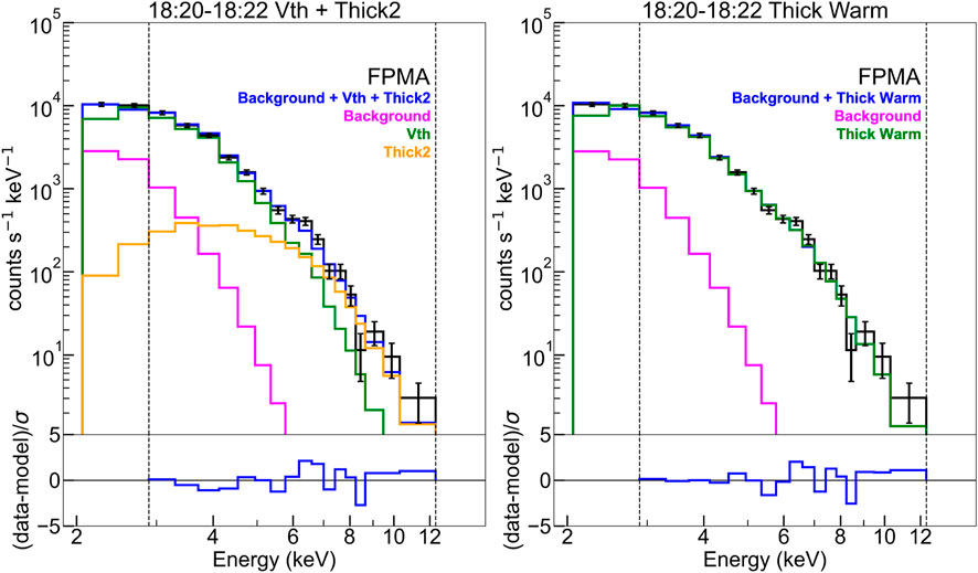
FIGURE 9. NuSTAR data from telescope FPMA was fit in OSPEX to model the electron distribution directly using the vth + thick2 (left) and thick warm (right) models. The thermal background taken at 18:40 UT is included, the fit is corrected for gain, and the count spectrum is pileup corrected. Modeling the electron distribution allows for a direct measurement of the cutoff energy parameter, which was found to be ≈8 keV.

TABLE 1

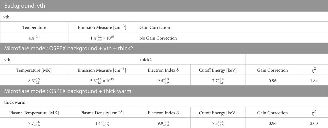
TABLE 1. Fit parameters for the background and OSPEX models, as well as the gain correction and fit statistic. All fits, including the background, include only the Western flaring region. The background was taken at 18:40 UT, after the flare. The thermal background component was held fixed for all spectral fitting of the source.

Thermal and non-thermal energies are calculated for the cold thick target model. The thermal energy may be calculated by assuming an isothermal plasma for each vth component. The thermal energy may be up to a few times greater than this isothermal approximation due to cooler components NuSTAR is not sensitive to (Aschwanden et al., 2015). The thermal energy is given by.

$U_T=3k_{B}T\sqrt{\text{EM}f\text{V}}\left[\text{erg}\right](1)$

$U_T\approx 1\times 10^{28}\left[\text{erg}\right](2)$

with the emission measure EM and temperature T taken from the vth fit. The filling factor f is assumed to be unity. The thermal energy is an order of magnitude estimate. For the thick warm calculation, $\sqrt{\text{EM}f\text{V}}$ is replaced with nV, with n representing the emission measure. The volume V was calculated from the AIA 94 Å images, solving for the area and converting to volume via A^3/2 = V. The AIA 94 Å data was cropped to the region used for spectroscopy, and thresholded to only the flaring region by subtracting the 18:40 UT background.

The non-thermal energy is found by multiplying the non-thermal power by the spectral observation window, in this case 2 minutes. If the electron spectrum F(ϵ) above the cutoff energy is assumed to be a power law of index δ, the non-thermal energy for the vth + thick2 model may be calculated as.

$\begin{array}{ll}\hfill U_N\left(E>E_C\right)& =P\left(E>E_C\right)\mathrm{\Delta }t={\int }_{E_C}^{\infty }\text{F}\left(ϵ\right)\text{E}dE\mathrm{\Delta }t\hfill \\ \hfill & \approx 1.6\times 10^{-9}\frac{\delta -1}{\delta -2}N{E}_C\mathrm{\Delta }t\left[\text{erg}\right]\hfill \end{array}(3)$

$U_N\left(E>E_C\right)=2.3_{-0.9}^{+0.9}\times 10^{28}\left[\text{erg}\right](4)$

with N representing the number of electrons per second, δ the electron spectral index, and E_C the cutoff energy—all parameters fit by OSPEX.

5 Modeling

5.1 RADYN simulations

The IRIS observations provide crucial information about the response of the plasma to the energy release in the lower atmosphere. At the same time, NuSTAR observations provide direct constraints on the energy distributions of the accelerated electrons in the corona. In order to find evidence for the physical mechanisms driving the flare, we run hydrodynamic simulations using the RADYN code (e.g., Carlsson and Stein, 1992; Allred et al., 2005; 2015; Carlsson et al., 2015), which solves the equation of radiative hydrodynamics on a 1-dimensional (1D) adaptive grid (Dorfi and Drury, 1987). A key property of RADYN is the ability to perform non-local thermodynamic equilibrium (non-LTE) radiative transfer for species which are important for chromospheric energy balance (e.g., H, He and Ca). Other atomic species are included as background continuum opacity sources (in LTE) using the Uppsala opacity package (Gustafsson, 1973). The radiative losses for optically thin lines are calculated using the CHIANTI 7.1 (Dere et al., 1997; Landi et al., 2013) database assuming ionization and thermal equilibrium.

RADYN simulates flare heating assuming different possible physical mechanisms: accelerated non-thermal electrons streaming from the corona to the chromosphere, whose propagation is treated using the Fokker-Planck equation (Allred et al., 2015); in-situ heating in the corona and consequent energy transport to the lower atmosphere via thermal conduction; or dissipation of Alfvén waves (Kerr et al., 2016). Since we have direct observations of accelerated electrons from NuSTAR, here we focus on the first mechanism.

We run simulations which covered a range of electron beam parameters and initial conditions of the flare loops, as summarized below.

• Energy flux (F) = 3 ⋅ 10⁸–5 ⋅ 10⁹ ergs s⁻¹ cm⁻² (3F8–5F9)

• Energy cut-off (E_C) = 4–9 keV

• Spectral index (δ) = 9–11

• Initial temperature at loop apex = 1MK and 3 MK (with apex densities = 10^8.7 and 10^9.6 cm⁻³ respectively)

We use values of E_C and δ which are close to those provided by the NuSTAR spectral analysis, within uncertainties. We simulate a broader range of values for the energy flux, since this parameter is not completely constrained by NuSTAR, as it depends also on the area over which the electrons deposit their energy (as discussed in Sect. 6). We use the same “plage-like” atmospheres presented in Polito et al. (2018), and we also assume half-loop lengths of 15 Mm. Our choice of loop length and initial temperatures is motivated by the larger parameter studies presented in Polito et al. (2018) and Testa et al. (2020). In particular, these studies have demonstrated that simulations with different loop lengths and the same initial temperature provide very similar trends (e.g., Figure A1 of Polito et al., 2018). Testa et al. (2014) and Polito et al. (2018) also showed that using hotter and denser initial loop atmospheres (e.g., 5 MK loop with apex density of ≈ 10¹⁰ cm³) results in less heating of the lower atmosphere for smaller events such as this B1 flare under study. Finally, given the uncertainty in the duration of the blue shifts in individual IRIS pixels due to the relatively long raster cadence of this observation, we assume here a heating duration of 10 s for simplicity, and we refer to future work for a more extended investigation of the effects of longer duration heating on the models (e.g., Testa et al., 2020; Cho et al., 2023).

5.2 Synthesis of IRIS spectral lines

We synthesize the emission of the IRIS Si iv spectral line using the values of density, temperature, and bulk velocity at each grid point and timestep from the RADYN simulations and atomic data from CHIANTI v.10 (Dere et al., 1997; Del Zanna et al., 2021), assuming photospheric abundances (Asplund et al., 2009) and equilibrium ionization. We follow Eq 1 of Polito et al. (2018) to convert the synthetic spectra to units of DN s⁻¹ pixel⁻¹. The time-velocity spectra described in Sect. 5.3 are then obtained by integrating the synthetic emission in each RADYN grid point along the loop as a function of time, assuming an exposure time of 1s and taking into account the instrumental broadening of 0.026 Å.

To synthesize the optically thick Mg ii and C ii spectra, we provide the input from our RADYN flare atmospheres (temperature, electron density, bulk velocity, hydrogen atomic level populations) as a function of time to the radiation transport code RH15D (Pereira and Uitenbroek, 2015). RH15D solves the equation of non-LTE radiation transport and atomic level populations and allows us to take into account the effects of partial redistribution (PRD), which can be important for the Mg ii lines (Leenaarts et al., 2013a). The NLTE radiation transport equations were solved for H, Mg ii and C ii, with additional species solved in LTE as sources of background opacity. We add a microturbulence of 7 km s⁻¹ as an additional source of line broadening mechanism in the chromosphere, consistent with the values reported in Carlsson et al. (2015), as well as a recent study by Sainz Dalda and De Pontieu (2022) based on inversions of IRIS Mg ii profiles during flares. The synthetic Mg ii and C ii NUV spectra were converted to IRIS count rates using the same procedure described in Polito et al. (2018); Testa et al. (2020); Polito et al. (2023).

5.3 Comparison between observations and models

Figure 10 (top panel) shows Si iv synthetic spectra as a function of velocity (x-axis) and time (y-axis) for different RADYN flare simulations, assuming an initial apex temperature of 1 MK, E_C = 8keV, δ = 10, and different values of energy flux, according to the legend. The vertical dotted white lines indicate the position of the line at rest (assuming the reference wavelength available in CHIANTI v.10), and negative values here indicate blueshifts. The time-velocity plots show that when the energy flux is below 5 ⋅ 10⁸ ergs s⁻¹ cm⁻² (5F8), the line is mostly blueshifted over time. On the other hand, as the flux energy increases, the line becomes more at-rest or red shifted. As described in detail in Polito et al. (2018), this different behavior is due to the fact that, in case of more gentle fluxes, the electrons can deposit their energy below the height formation of Si iv–and thus driving the Si iv evaporation–for a longer time. In these simulations it takes longer for the loop density to rise, meaning that the electrons can deposit energy in the lower atmosphere for a longer time. In fact, when the density is high enough, the electrons get stopped at higher heights and eventually drive a downflow of Si iv plasma. This shift from upflow to downflow happens much quicker in simulations with stronger energy flux (see Polito et al., 2018, for more details).

FIGURE 10

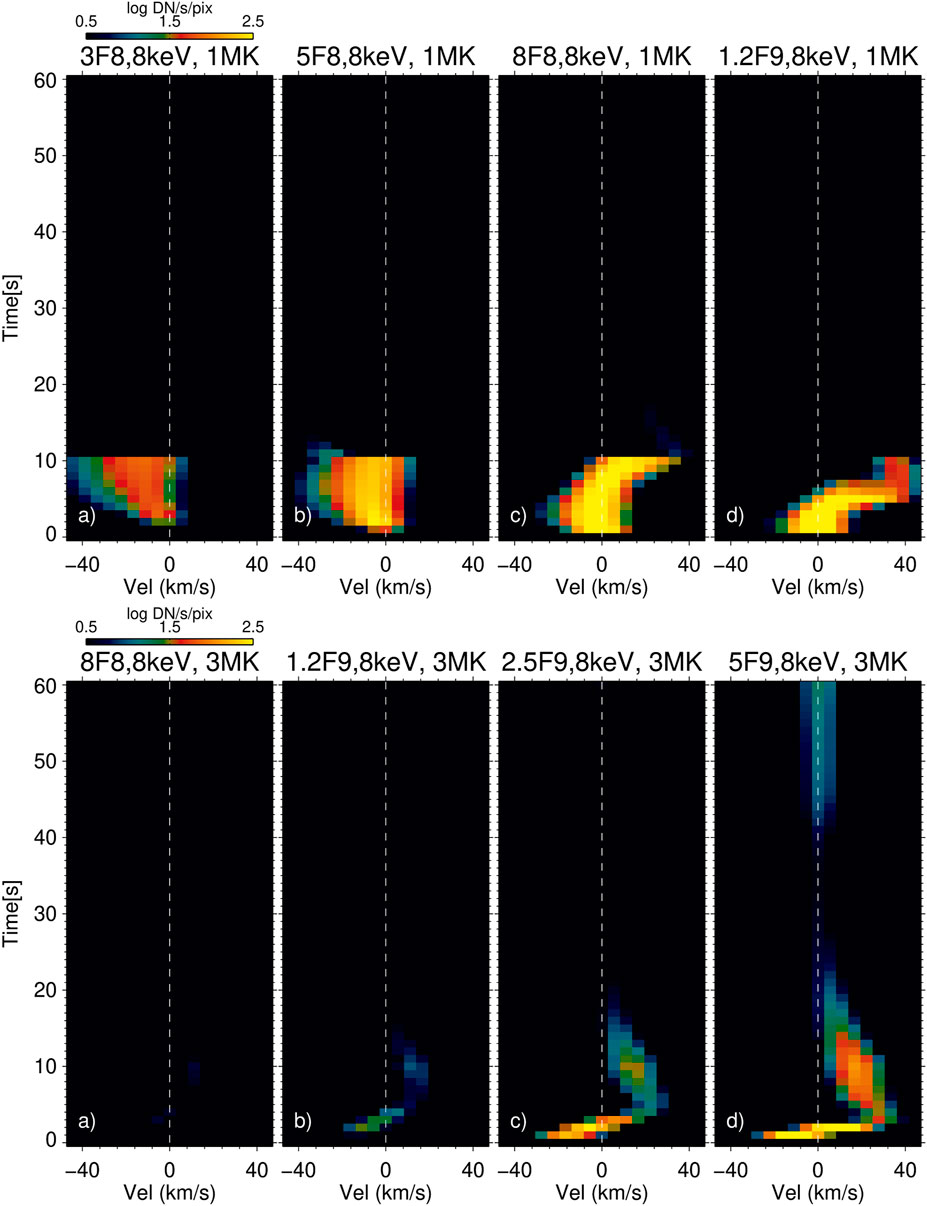
FIGURE 10. Time-velocity synthetic spectra of Si iv for different RADYN flare simulations. Top panels: simulations with an apex temperature of 1 MK, E_C = 8keV, δ = 10 keV, in different F = 3F8 (A), 5F8 (B), 8F8 (C) and 1.2F9 (D). Bottom panels: same as top panels, with initial apex temperature of 3 MK, and F = 8F8 (A), 1.2F9 (B), 2.5F9 (C) and 5F9 (D).

Figure 10 (bottom panels) shows Si iv synthetic spectra for models with an initial apex temperature of 3 MK. As also discussed in Polito et al. (2018), this hotter initial atmosphere is also denser (with apex density 10^9.6 cm⁻³ compared to 10^8.7 cm⁻³ for the 1MK loop), meaning that the electrons need comparatively higher energy to be able to heat the transition region and therefore drive an increase of intensity and brightenings in the Si iv line. This phenomenon is illustrated in Figure 10A), which shows that an energy flux of at least 1.2 ⋅ 10⁹ ergs s⁻¹ cm⁻² (1.2F9) is needed to drive a response in the Si iv line. These results demonstrate that in order to reproduce the Si iv blueshift, one needs a certain combination of parameters for the electron beam distribution, which will also depend on the initial conditions.

Figure 11 shows a summary of Si iv Doppler shift velocities based on moment calculation for different models. Panel a) summarizes the Si iv Doppler shift velocity at the maximum intensity during the simulation, while panel b) shows the maximum blue shift velocity during the simulation. For both panels, we only consider spectra where the Si iv line is above a detection threshold of 10 DN for the total intensity of the line. For some simulations there is no associated data point in Figure 11B), which means that the Si iv line does not exhibit blue shifts in the detectable spectra. Figure 11 also shows that, in order to reproduce a significant (of 10 km s⁻¹ or larger) Si iv blueshift for the range of E_C obtained from the NuSTAR observations, including uncertainties (i.e. 7–9 keV), we need an energy below ≈8 ⋅ 10⁸ ergs s⁻¹ cm⁻² (8F8) for the 1MK loop or ≈5 ⋅ 10⁹ ergs s⁻¹ cm⁻² (5F9) for the 3MK loop. Further, we note that for the 5F9 model, the maximum blueshift does not occur in the brightest spectrum of the simulation. Finally, Figure 11B) shows the impact of the initial temperature (and density) of the loop atmosphere on the magnitude of the Doppler shifts, with stronger Si iv blueshift values being observed in simulations with an initial lower temperature loop. This behavior was also discussed in Polito et al. (2018) and suggests that, although the observed values of blueshifts are slightly larger (≈-25–30 km s⁻¹) than the maximum blueshifts observed in the simulations with the 3MK loop, this might be due to some extent to the details of the initial physical conditions of the loops.

FIGURE 11

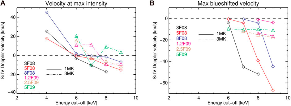
FIGURE 11. Summary of Si iv Doppler shifts as a function of E_C for different RADYN models. Panel (A) shows the line Doppler shifts at the time of maximum Si iv intensity during the simulation. Panel (B) shows the largest blueshift for each simulation. In both cases, we only analyze spectra which are strong enough to be observed (with total intensity greater than 10DN).

Previous work has shown that studying the response of the atmosphere to the flare heating by combining IRIS spectral lines formed at different heights from the chromosphere to the transition region, we can obtain even stricter constraints on the models (Polito et al., 2018; Testa et al., 2020). With this motivation in mind, we investigate in more detail the behavior of the chromospheric lines for those models where we succeed in reproducing the Si iv blueshifts. Figure 12 (top panels) shows synthetic spectra for the Si iv (Panel a), C ii (Panel b), Mg ii (Panel c) and Mg ii triplet (Panel d) lines as a function of velocity and time for the 5F8 model with E_C = 8 keV, δ = 10 and initial loop apex temperature of 3MK. The bottom panels show the same quantities for the 2.5F9 flare model with E_C = 8 keV, δ = 10 and initial loop apex temperature of 3MK. Figure A2 in the Appendix also show the synthetic spectra of the IRIS lines for the 1.2F9 model and 3 MK loop. While these three models can to some extent explain the observed Si iv blueshifts, they are characterized by different behaviors in the synthetic spectra of the chromospheric lines. In particular, the Mg ii k and triplet chromospheric lines in the simulations with the 1 MK loop are characterized by a deeper central reversal (Figure 12, top panels c) and d)). A less pronounced center reversal (which is still deeper than that in the observed spectra) is also seen in the 1.2F9 model and 3 MK loop (Figure A2). On the other hand, the chromospheric spectra in the 2.5F9 flare model with the 3MK loop (Figure 12, bottom panels c) and d)) more closely resemble the key characteristics of the observed spectra. One main difference that remains is that, in all of the three models, the C ii line appears to be red shifted or stationary, while in the observations the line is blueshifted. Another difference between models and observations is in the values of line width, which are smaller in the models than the observations. Such discrepancies are well-known and were discussed in detail in e.g. Testa et al. (2020), Cho et al. (2023). In particular, these previous studies pointed out the difficulty associated with comparing the results of a single loop model with observed spectral lines in one IRIS pixel, where heating episodes from many individual loop strands (possibly also with different physical conditions) might overlap. In addition, physical mechanisms such as turbulence and waves, which are missing from our models, may contribute to the discrepancy between the observed and simulated line widths.

FIGURE 12

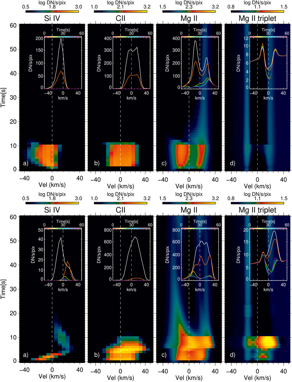
FIGURE 12. Top panels: Synthetic spectra from RADYN and RH simulations for the 5F8 flare model with E_C = 8 keV, δ = 10 and initial loop apex temperature of 1MK. The four panels show the: Si iv (Panel A), C ii (Panel B), Mg ii (Panel C) and Mg ii triplet (Panel D) lines as a function of velocity and time. The insert on each panel shows the spectra averaged in time with a cadence of 8s, as indicated by the legend. Bottom panels: Same plots for the 2.5F9 flare model with E_C = 8 keV, δ = 10 and initial loop apex temperature of 3MK.

In summary, despite their limitations, the models with an initial temperature of 3MK and energy flux in the range of 1.2–2.5F9 are capable of reproducing qualitative observational characteristics of the flare spectra (e.g., Si iv blueshift, lack of Mg ii k deep central reversal and presence of increased Mg ii triplet emission). We note that the initial higher temperature for the flare loops is more consistent also with the background temperature observed by NuSTAR of ≈ 4MK.

The comparison discussed here demonstrates how the models can provide a useful tool to constrain the properties of the heating. In order to compare the simulations with the results of the NuSTAR X-ray spectral analysis, we need to estimate the area over which the electrons might deposit their energy in the lower atmosphere. In Sect.6 we discuss how to derive this value using magnetic field extrapolations, while in Sect. 7 we compare both UV and X-ray observations with the predictions of the models and summarize our conclusions.

6 Magnetic field extrapolation

Figure 13 shows an overview of the three-dimensional (3D) magnetic field modeling of the AR 12821 under study. In particular, panels a), b) and c) show: the radial component of the photospheric magnetic field from HMI, AIA 94 Å and IRIS SJI 1330 Å images respectively for context to the magnetic field extrapolation. Panels d), e) and f) show a nonlinear force-free field (NLFFF) extrapolation model of the active region with different line-of-sight views. The HMI radial magnetic field in panel a) and vector magnetogram data used for the extrapolation are taken just before the beginning of the flare activity in the AR complex 12820/12821 as to minimize the possible impact on the photosphere. The images in panels b) and c) are taken at the same time as that in Figure 14. The extrapolation was performed using the optimization algorithm from Wiegelmann et al. (2012), with a Cartesian grid of 970 km per pixel.

FIGURE 13

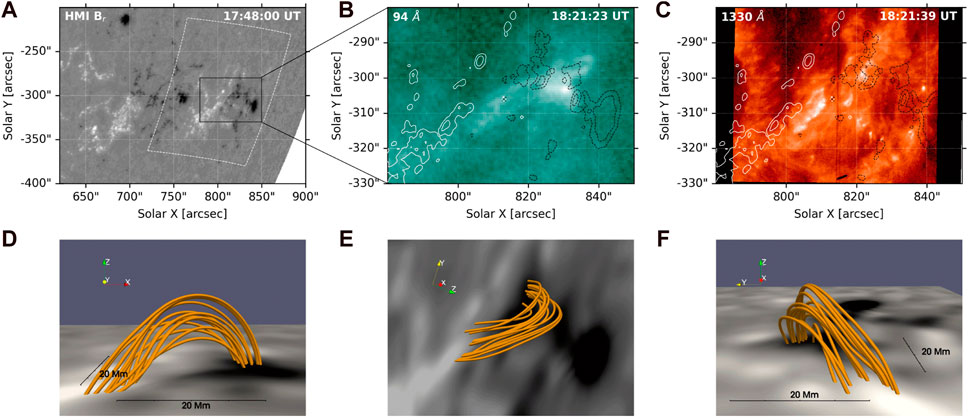
FIGURE 13. 3D modeling of the NOAA 12821 Active region. Panel (A) Radial component of the photospheric magnetic field strength obtained at 17:48 UT, with the boundary data region for magnetic field extrapolation denoted by a white dashed box. Panel (B–C) AIA 94 Å image and IRIS SJI image in 1,330 Å filter, with their FOV indicated by a black solid box in panel (A). Magnetic field strength contours of ±500 and ±1,000 Gauss overlaid, with the positive and negative polarity shown as white and black lines, respectively. Panel (D–F) Nonlinear force-free field (NLFFF) extrapolation model of the AR, viewed from Y-axis, line-of-sight, and X-axis perspectives. X- and Y-axes represent heliographic longitude and latitude on the solar disk, respectively, while Z-axis points radially from the solar center.

FIGURE 14

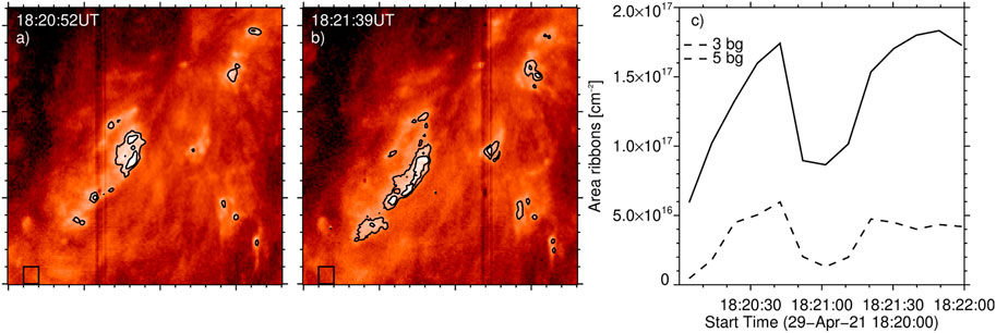
FIGURE 14. Estimation of the ribbon area from the IRIS UV images. Panel (A, B) show the SJI 1330 Å images at two time intervals during the flare. The contours show the intensity above 3 and 5 (dotted line) times the intensity of a chosen background area within the active region, which is highlighted by the small black boxes. Panel (C) shows the same contour areas as a function of time during the NuSTAR observation.

The comparison between the extrapolation and the AIA and IRIS SJI images confirms that the event under study occurs in the eastern part of the active region. This comparison has enabled us to determine the magnetic connectivity of the loops visible in the AIA 94 Å images and the ribbons observed by IRIS. The extrapolation also suggests that the flare loops are rooted between the larger and more elongated ribbon observed in the IRIS SJI images at approximately 810″ in solar X direction, and the more fragmented brightenings located to the west at around 820′′.

Figure 14 (panels a) and b)) shows the IRIS SJI 1330 Å images at two time intervals during the flare, with overlaid contours highlighting the image intensity above 3 and 5 (dotted line) times a background intensity. The location where we measure the background is indicated by the small black boxes in panels a) and b) and is chosen to be within the AR but outside the ribbons. After comparison between these images and Figure 13 we suggest that the ribbon area identified by the contours roughly represents the region where the flare loops are rooted. Further, panel c) shows the time evolution of the contour areas. We take these values as an approximation of the area over which the electrons may deposit their energy over time. Such assumption is not perfect and provides just an order of magnitude estimate, but we cannot obtain a more accurate estimate since the NuSTAR spatial resolution does not allow us to measure the area of the X-ray footpoints. Using this method, we find that the estimated area A_min/max for the ribbons is ≈4.6 ⋅ 10¹⁵ to 1.8 ⋅ 10¹⁷ cm².

7 Discussion and conclusion

We have analyzed rare coordinated IRIS and NuSTAR observations of a small B-class microflare on 29 April 2021, which provide independent diagnostics of non-thermal particles and therefore a unique opportunity to constrain the properties of accelerated particles in small heating events. The IRIS slit observes the largest flare ribbon, and analysis of the IRIS spectral lines show peculiar spectral characteristics in some of the pixels (e.g., Si iv blueshift and enhanced Mg ii triplet emission), which, as extensively described in our previous works (e.g., Testa et al., 2014; Polito et al., 2018; Testa et al., 2020; Cho et al., 2023), are indirect signatures of the presence of non-thermal electrons in the lower atmosphere. Here we focus on the spectra characterized by Si iv blueshifts because those are the unique spectral signatures of non-thermal particles, but we note that Si iv redshifts are also observed in other locations along the ribbon (and can be also due to non-thermal particles under certain conditions; see, e.g., Testa et al., 2014; Polito et al., 2018; Testa et al., 2020). Direct confirmation for the presence of accelerated electrons in the corona is independently provided by the NuSTAR spectral investigation which observes the hard X-ray emission.

We compare the IRIS spectral observations with the predictions of RADYN hydrodynamic models assuming flare heating by accelerated electron beams, and use the measurements of the electron beam parameters from NuSTAR to guide our parameter space of the simulations. In particular, we simulate models with a range of low-energy cutoff and spectral index values that are consistent with those observed with NuSTAR. As mentioned earlier, the only parameter that we cannot directly compare with the models is the electron energy flux, as that requires an estimation of the area over which the electrons deposit their energy, which is not known with great accuracy. In Sect. 6, we provide some order of magnitude estimates for such area based on the IRIS UV images. Using those values and the energy flux measured by NuSTAR, we obtain the following values of energy flux F for the electron beams:

$E_{\mathit{NuSTAR}}=1.9\cdot 10^{26}ergs{s}^{-1}(5)$

$\begin{array}{ll}\hfill F& =\frac{E_{\mathit{NuSTAR}}}{A_{\mathit{min}/\mathit{max}}}=\frac{1.9\cdot 10^{26}}{4.6\cdot 10^{15}/1.8\cdot 10^{17}}ergs{s}^{-1}c{m}^{-2}\hfill \\ \hfill & =1.0\cdot 10^9-4.1\cdot 10^{10}ergs{s}^{-1}c{m}^{-2}\hfill \end{array}(6)$

The comparison between the IRIS transition region and chromospheric line spectra and the RADYN simulations suggest that the best candidate models to explain the observations are electron-beam heating models with F ≈ 1.2–2.5 ⋅ 10⁹ ergs s⁻¹ cm⁻² and an initial apex temperature of 3MK. These values are consistent with the lower range of F independently estimated from NuSTAR in Eq. 6. If non-thermal energy calculations for the warm thick target model are used, the computed NuSTAR energy flux range is 1.6 ⋅ 10⁹–9.0 ⋅ 10¹⁰, which still overlaps the energy flux range of the electron-beam heating models. A direct comparison of the energy estimate from the RADYN simulations that best reproduce the IRIS observations and that obtained by NuSTAR can be affected by a number of factors, including but not limited to: (1) the uncertainty in the estimate of the ribbon area, as discussed in Sect. 6; (2) difference between energy released in the corona (measured by NuSTAR) and energy dissipated in the ribbons (where IRIS is observing); (3) inhomogeneities on how the energy is distributed in different locations along the ribbons (also suggested by the different behavior of the Si iv Doppler shifts). We should also mention the different timescales involved in our analysis: we integrated the NuSTAR spectra over a period of about 2 min to increase the signal-to-noise ratio, while the IRIS exposure time is 8 s with a raster cadence of ≈ 75 s. Therefore, it is possible that the energy release varies during the 2 min of the NuSTAR observations. HXR observations with high enough sensitivity to detect small energetic events at significantly higher cadence are not available at the moment and would be highly desirable in the future. Despite these possible sources of uncertainty, we find a reasonable agreement between the energy estimate between different methods.

In conclusion, this work demonstrates that combining UV and X-ray spectral observations from IRIS and NuSTAR with state-of-art simulations can provide crucial diagnostics of flare heating models. We have also presented a consistent picture based on independent measurements of non-thermal particle acceleration in the corona and the response of the lower atmospheric plasma to the non-thermal energy deposition.

Given the difficulty associated with coordinating different instruments, including a single-slit spectrograph, catching a flare in the right location and at the same time, it is not surprising that this is the first of such studies that we were able to perform. We hope to expand this work in the near future by obtaining larger statistics of IRIS and NuSTAR coordinated events and by comparing the observations with an extended range of models, including longer duration heating and different initial conditions for the loops (following other recent broader investigations such as that of Testa et al., 2020; Cho et al., 2023).

Data availability statement

Publicly available datasets were analyzed in this study. This data can be found here: https://iris.lmsal.com, https://heasarc.gsfc.nasa.gov/docs/nustar/nustar_archive.html, https://sdo.gsfc.nasa.gov/data/aiahmi/.

Author contributions

VP led the analysis of the IRIS observations and modeling and MP led the analysis of the NuSTAR observations. LG assisted MP on the NuSTAR analysis. PT and Dr. Kathy KR assisted VP on the IRIS and AIA analysis, and PT also assisted with the interpretation of RADYN models and their comparison with the observations. XS performed the magnetic field extrapolation, and SY worked on the 3D visualization of the extrapolation results. JD acquired the NuSTAR data used in this manuscript. All authors contributed to the article and approved the submitted version.

Funding

VP, SY, KR and XS acknowledge support from NASA Heliophysics System Observatory Connect Grant # 80NSSC20K1283. VP also acknowledges support from NASA ROSES Heliophysics Guest Investigator program (Grant# NASA 80NSSC20K0716) and from NASA under contract NNG09FA40C(IRIS). LG and MP acknowledge the NSF CAREER grant AGS1752268 and NASA Guest Observer grant 80NSSC21K0135. PT was supported by contract 8100002705 (IRIS) to the Smithsonian Astrophysical Observatory, and NASA grant 80NSSC20K1272. SY and VP acknowledge support from NASA Early Career Investigator Program (Grant# NASA 80NSSC21K0623). JD’s research was supported by an appointment to the NASA Postdoctoral Program at the NASA Goddard Space Flight Center, administered by Oak Ridge Associated Universities under contract with NASA. Resources supporting this work were provided by the NASA High-End Computing (HEC) Program through the NASA Advanced Supercomputing (NAS) Division at Ames Research Center.

Acknowledgments

CHIANTI is a collaborative project involving George Mason University, the University of Michigan (United States), and the University of Cambridge (United Kingdom). AIA and HMI data are courtesy of NASA/SDO and the AIA and HMI science team. IRIS is a NASA small explorer mission developed and operated by LMSAL with mission operations executed at NASA Ames Research center and major contributions to downlink communications funded by ESA and the Norwegian Space Centre. This paper made use of data from the NuSTAR mission, a project led by the California Institute of Technology, managed by the Jet Propulsion Laboratory, funded by the National Aeronautics and Space Administration.

Conflict of interest

The authors declare that the research was conducted in the absence of any commercial or financial relationships that could be construed as a potential conflict of interest.

Publisher’s note

All claims expressed in this article are solely those of the authors and do not necessarily represent those of their affiliated organizations, or those of the publisher, the editors and the reviewers. Any product that may be evaluated in this article, or claim that may be made by its manufacturer, is not guaranteed or endorsed by the publisher.

Supplementary material

The Supplementary Material for this article can be found online at: https://www.frontiersin.org/articles/10.3389/fspas.2023.1214901/full#supplementary-material

Footnotes

¹https://www.isas.jaxa.jp/home/solar/hinode_op/hop.php?hop=0409

References

Allred, J. C., Hawley, S. L., Abbett, W. P., and Carlsson, M. (2005). Radiative hydrodynamic models of the optical and ultraviolet emission from solar flares. Apj 630, 573–586. doi:10.1086/431751

CrossRef Full Text | Google Scholar

Allred, J. C., Kowalski, A. F., and Carlsson, M. (2015). A unified computational model for solar and stellar flares. Apj 809, 104. doi:10.1088/0004-637X/809/1/104

CrossRef Full Text | Google Scholar

Arnaud, K. A. (1996). “Xspec: the first ten years,” in Astronomical data analysis software and systems V of astronomical society of the pacific conference series. Editors G. H. Jacoby, and J. Barnes, 101, 17.

Google Scholar

Aschwanden, M. J., Boerner, P., Ryan, D., Caspi, A., McTiernan, J. M., and Warren, H. P. (2015). Global energetics of solar flares: ⅠⅠ. Thermal energies. Apj 802, 53. doi:10.1088/0004-637X/802/1/53

CrossRef Full Text | Google Scholar

Asplund, M., Grevesse, N., Sauval, A. J., and Scott, P. (2009). The chemical composition of the Sun. ARA&A 47, 481–522. doi:10.1146/annurev.astro.46.060407.145222

CrossRef Full Text | Google Scholar

Benz, A. O. (2008). Flare observations. Living Rev. Sol. Phys. 5, 1. doi:10.12942/lrsp-2008-1

PubMed Abstract | CrossRef Full Text | Google Scholar

Boerner, P., Edwards, C., Lemen, J., Rausch, A., Schrijver, C., Shine, R., et al. (2012). Initial calibration of the atmospheric imaging assembly (AIA) on the solar Dynamics observatory (SDO). Sol. Phys. 275, 41–66. doi:10.1007/s11207-011-9804-8

CrossRef Full Text | Google Scholar

Carlsson, M., Leenaarts, J., and De Pontieu, B. (2015). What do IRIS observations of Mg II k tell us about the solar plage chromosphere? ApJ 809, L30. doi:10.1088/2041-8205/809/2/L30

CrossRef Full Text | Google Scholar

Carlsson, M., and Stein, R. F. (1992). Non-LTE radiating acoustic shocks and CA II K2V bright points. ApJ 397, L59–L62. doi:10.1086/186544

CrossRef Full Text | Google Scholar

Caspi, A., Krucker, S., and Lin, R. P. (2014). Statistical properties of super-hot solar flares. ApJ 781, 43. doi:10.1088/0004-637X/781/1/43

CrossRef Full Text | Google Scholar

Cho, K., Testa, P., De Pontieu, B., and Polito, V. (2023). A statistical study of IRIS observational signatures of nanoflares and nonthermal particles. ApJ 945, 143. doi:10.3847/1538-4357/acb7da

CrossRef Full Text | Google Scholar

Christe, S., Hannah, I. G., Krucker, S., McTiernan, J., and Lin, R. P. (2008). RHESSI microflare statistics. I. Flare-finding and frequency distributions. ApJ 677, 1385–1394. doi:10.1086/529011

CrossRef Full Text | Google Scholar

Cooper, K., Hannah, I. G., Grefenstette, B. W., Glesener, L., Krucker, S., Hudson, H. S., et al. (2020). NuSTAR observation of a minuscule microflare in a solar active region. ApJ 893, L40. doi:10.3847/2041-8213/ab873e

CrossRef Full Text | Google Scholar

Cooper, K., Hannah, I. G., Grefenstette, B. W., Glesener, L., Krucker, S., Hudson, H. S., et al. (2021). NuSTAR observations of a repeatedly microflaring active region. MNRAS 507, 3936–3951. doi:10.1093/mnras/stab2283

CrossRef Full Text | Google Scholar

De Pontieu, B., Polito, V., Hansteen, V., Testa, P., Reeves, K. K., Antolin, P., et al. (2021). A new view of the solar Interface region from the Interface region imaging spectrograph (IRIS). Sol. Phys. 296, 84. doi:10.1007/s11207-021-01826-0

CrossRef Full Text | Google Scholar

De Pontieu, B., Title, A. M., Lemen, J. R., Kushner, G. D., Akin, D. J., Allard, B., et al. (2014). The Interface region imaging spectrograph (IRIS). Sol. Phys. 289, 2733–2779. doi:10.1007/s11207-014-0485-y

CrossRef Full Text | Google Scholar

Del Zanna, G., Dere, K. P., Young, P. R., and Landi, E. (2021). CHIANTI—an atomic database for emission lines. XVI. Version 10, further extensions. ApJ 909, 38. doi:10.3847/1538-4357/abd8ce

CrossRef Full Text | Google Scholar

Del Zanna, G. (2013). The multi-thermal emission in solar active regions. A&A 558, A73. doi:10.1051/0004-6361/201321653

CrossRef Full Text | Google Scholar

Dennis, B. R., Veronig, A., Schwartz, R. A., Sui, L., Tolbert, A. K., Zarro, D. M., et al. (2003). The neupert effect and new RHESSI measures of the total energy in electrons accelerated in solar flares. Adv. Space Res. 32, 2459–2464. doi:10.1016/S0273-1177(03)00884-6

CrossRef Full Text | Google Scholar

Dere, K. P., Landi, E., Mason, H. E., Monsignori Fossi, B. C., and Young, P. R. (1997). Chianti - an atomic database for emission lines. A&AS 125, 149–173. doi:10.1051/aas:1997368

CrossRef Full Text | Google Scholar

Dorfi, E. A., and Drury, L. O. (1987). Simple adaptive grids for 1-D initial value problems. J. Comput. Phys. 69, 175–195. doi:10.1016/0021-9991(87)90161-6

CrossRef Full Text | Google Scholar

Duncan, J., Glesener, L., Grefenstette, B. W., Vievering, J., Hannah, I. G., Smith, D. M., et al. (2021). NuSTAR observation of energy release in 11 solar microflares. ApJ 908, 29. doi:10.3847/1538-4357/abca3d

CrossRef Full Text | Google Scholar

Fletcher, L., Dennis, B. R., Hudson, H. S., Krucker, S., Phillips, K., Veronig, A., et al. (2011). An observational overview of solar flares. Space Sci. Rev. 159, 19–106. doi:10.1007/s11214-010-9701-8

CrossRef Full Text | Google Scholar

Glesener, L., Krucker, S., Duncan, J., Hannah, I. G., Grefenstette, B. W., Chen, B., et al. (2020). Accelerated electrons observed down to <7 keV in a NuSTAR solar microflare. ApJ 891, L34. doi:10.3847/2041-8213/ab7341

CrossRef Full Text | Google Scholar

Glesener, L., Krucker, S., Hannah, I. G., Hudson, H., Grefenstette, B. W., White, S. M., et al. (2017). NuSTAR hard X-ray observation of a sub-A class solar flare. ApJ 845, 122. doi:10.3847/1538-4357/aa80e9

CrossRef Full Text | Google Scholar

Grefenstette, B. W., Glesener, L., Krucker, S., Hudson, H., Hannah, I. G., Smith, D. M., et al. (2016). The first focused hard X-ray images of the Sun with NuSTAR. ApJ 826, 20. doi:10.3847/0004-637X/826/1/20

CrossRef Full Text | Google Scholar

Gustafsson, B. (1973). Uppsala astron. Obs. Ann. 5.

Google Scholar

Hannah, I. G., Christe, S., Krucker, S., Hurford, G. J., Hudson, H. S., and Lin, R. P. (2008). RHESSI microflare statistics. II. X-ray imaging, spectroscopy, and energy distributions. ApJ 677, 704–718. doi:10.1086/529012

CrossRef Full Text | Google Scholar

Hannah, I. G., Kleint, L., Krucker, S., Grefenstette, B. W., Glesener, L., Hudson, H. S., et al. (2019). Joint X-ray, EUV, and UV observations of a small microflare. ApJ 881, 109. doi:10.3847/1538-4357/ab2dfa

CrossRef Full Text | Google Scholar

Harrison, F. A., Craig, W. W., Christensen, F. E., Hailey, C. J., Zhang, W. W., Boggs, S. E., et al. (2013). The nuclear spectroscopic telescope array (NuSTAR) high-energy X-ray mission. ApJ 770, 103. doi:10.1088/0004-637X/770/2/103

CrossRef Full Text | Google Scholar

Hudson, H. S. (1991). Solar flares, microflares, nanoflares, and coronal heating. Sol. Phys. 133, 357–369. doi:10.1007/BF00149894

CrossRef Full Text | Google Scholar

Kerr, G. S., Fletcher, L., Russell, A. J. B., and Allred, J. C. (2016). Simulations of the Mg II k and Ca II 8542 lines from an AlfvÉn wave-heated flare chromosphere. ApJ 827, 101. doi:10.3847/0004-637X/827/2/101

CrossRef Full Text | Google Scholar

Koglin, J. E., An, H., Barrière, N., Brejnholt, N. F., Christensen, F. E., Craig, W. W., et al. (2011). “First results from the ground calibration of the NuSTAR flight optics,” in Society of photo-optical instrumentation engineers (SPIE) conference series of society of photo-optical instrumentation engineers (SPIE) conference series. Editors S. L. O’Dell, and G. Pareschi, 8147, 81470J. doi:10.1117/12.895279

CrossRef Full Text | Google Scholar

Landi, E., Young, P. R., Dere, K. P., Del Zanna, G., and Mason, H. E. (2013). CHIANTI—an atomic database for emission lines. XIII. Soft X-ray improvements and other changes. ApJ 763, 86. doi:10.1088/0004-637X/763/2/86

CrossRef Full Text | Google Scholar

Leenaarts, J., a, T. M. D., Carlsson, M., Uitenbroek, H., and De Pontieu, B. (2013a). The Formation of iris diagnostics. I. A quintessential model atom of Mg II and general formation properties of the Mg II h&k lines. ApJ 772, 89. doi:10.1088/0004-637X/772/2/89

CrossRef Full Text | Google Scholar

Leenaarts, J., Pereira, T. M. D., Carlsson, M., Uitenbroek, H., and De Pontieu, B. (2013b). The Formation of IRIS diagnostics. II. The formation of the Mg II h&k lines in the solar atmosphere. ApJ 772, 90. doi:10.1088/0004-637X/772/2/90

CrossRef Full Text | Google Scholar

Lemen, J. R., Title, A. M., Akin, D. J., Boerner, P. F., Chou, C., Drake, J. F., et al. (2012). The atmospheric imaging assembly (AIA) on the solar Dynamics observatory (SDO). Sol. Phys. 275, 17–40. doi:10.1007/s11207-011-9776-8

CrossRef Full Text | Google Scholar

Lin, R. P., Dennis, B. R., Hurford, G. J., Smith, D. M., Zehnder, A., Harvey, P. R., et al. (2002). The reuven ramaty high-energy solar spectroscopic imager (RHESSI). Sol. Phys. 210, 3–32. doi:10.1023/A:1022428818870

CrossRef Full Text | Google Scholar

Madsen, K. K., Harrison, F. A., Markwardt, C. B., An, H., Grefenstette, B. W., Bachetti, M., et al. (2015). Calibration of the NuSTAR high-energy focusing X-ray telescope. ApJS 220, 8. doi:10.1088/0067-0049/220/1/8

CrossRef Full Text | Google Scholar

Martínez-Sykora, J., De Pontieu, B., Testa, P., and Hansteen, V. (2011). Forward modeling of emission in solar Dynamics observatory/atmospheric imaging assembly passbands from dynamic three-dimensional simulations. ApJ 743, 23. doi:10.1088/0004-637X/743/1/23

CrossRef Full Text | Google Scholar

Neupert, W. M. (1968). Comparison of solar X-ray line emission with microwave emission during flares. ApJ 153, L59. doi:10.1086/180220

CrossRef Full Text | Google Scholar

O’Dwyer, B., Del Zanna, G., Mason, H. E., Weber, M. A., and Tripathi, D. (2010). SDO/AIA response to coronal hole, quiet Sun, active region, and flare plasma. A&A 521, A21. doi:10.1051/0004-6361/201014872

CrossRef Full Text | Google Scholar

Parker, E. N. (1988). Nanoflares and the solar X-ray corona. ApJ 330, 474. doi:10.1086/166485

CrossRef Full Text | Google Scholar

Pereira, T. M. D., Carlsson, M., De Pontieu, B., and Hansteen, V. (2015). The Formation of IRIS diagnostics. IV. The Mg II triplet lines as a new diagnostic for lower chromospheric heating. ApJ 806, 14. doi:10.1088/0004-637X/806/1/14

CrossRef Full Text | Google Scholar

Pereira, T. M. D., and Uitenbroek, H. (2015). RH 1.5D: a massively parallel code for multi-level radiative transfer with partial frequency redistribution and zeeman polarisation. A&A 574, A3. doi:10.1051/0004-6361/201424785

CrossRef Full Text | Google Scholar

Pesnell, W. D., Thompson, B. J., and Chamberlin, P. C. (2012). The solar Dynamics observatory (SDO). Sol. Phys. 275, 3–15. doi:10.1007/s11207-011-9841-3

CrossRef Full Text | Google Scholar

Polito, V., Kerr, G. S., Xu, Y., Sadykov, V. M., and Lorincik, J. (2023). Solar flare ribbon fronts. I. Constraining flare energy deposition with IRIS spectroscopy. ApJ 944, 104. doi:10.3847/1538-4357/acaf7c

CrossRef Full Text | Google Scholar

Polito, V., Reep, J. W., Reeves, K. K., Simões, P. J. A., Dudík, J., Del Zanna, G., et al. (2016). Simultaneous iris andhinode/eis observations and modeling of the 2014 october 27 X2.0 class flare. Astrophysical J. 816, 89. doi:10.3847/0004-637X/816/2/89

CrossRef Full Text | Google Scholar

Polito, V., Testa, P., Allred, J., De Pontieu, B., Carlsson, M., Pereira, T. M. D., et al. (2018). Investigating the response of loop plasma to nanoflare heating using RADYN simulations. ApJ 856, 178. doi:10.3847/1538-4357/aab49e

CrossRef Full Text | Google Scholar

Reale, F., Testa, P., Petralia, A., and Graham, D. R. (2019a). Impulsive coronal heating from large-scale magnetic rearrangements: from IRIS to SDO/AIA. ApJ 882, 7. doi:10.3847/1538-4357/ab304f

CrossRef Full Text | Google Scholar

Reale, F., Testa, P., Petralia, A., and Kolotkov, D. Y. (2019b). Large-amplitude quasiperiodic pulsations as evidence of impulsive heating in hot transient loop systems detected in the EUV with SDO/AIA. ApJ 884, 131. doi:10.3847/1538-4357/ab4270

CrossRef Full Text | Google Scholar

Rubio da Costa, F., Kleint, L., Petrosian, V., Liu, W., and Allred, J. C. (2016). Data-driven radiative hydrodynamic modeling of the 2014 march 29 X1.0 solar flare. ApJ 827, 38. doi:10.3847/0004-637X/827/1/38

CrossRef Full Text | Google Scholar

Sainz Dalda, A., and De Pontieu, B. (2022). Chromospheric thermodynamic conditions from inversions of complex Mg II h&k profiles observed in flares. arXiv e-prints , arXiv:2211.05459.

Google Scholar

Scherrer, P. H., Schou, J., Bush, R. I., Kosovichev, A. G., Bogart, R. S., Hoeksema, J. T., et al. (2012). The helioseismic and magnetic imager (HMI) investigation for the solar Dynamics observatory (SDO). Sol. Phys. 275, 207–227. doi:10.1007/s11207-011-9834-2

CrossRef Full Text | Google Scholar

Shibata, K., and Magara, T. (2011). Solar flares: magnetohydrodynamic processes. Living Rev. Sol. Phys. 8, 6. doi:10.12942/lrsp-2011-6

CrossRef Full Text | Google Scholar

Testa, P., De Pontieu, B., Allred, J., Carlsson, M., Reale, F., Daw, A., et al. (2014). Evidence of nonthermal particles in coronal loops heated impulsively by nanoflares. Science 346, 1255724. doi:10.1126/science.1255724

PubMed Abstract | CrossRef Full Text | Google Scholar

Testa, P., De Pontieu, B., Martínez-Sykora, J., DeLuca, E., Hansteen, V., Cirtain, J., et al. (2013). Observing coronal nanoflares in active region moss. ApJ 770, L1. doi:10.1088/2041-8205/770/1/L1

CrossRef Full Text | Google Scholar

Testa, P., Polito, V., and De Pontieu, B. (2020). IRIS observations of short-term variability in moss associated with transient hot coronal loops. ApJ 889, 124. doi:10.3847/1538-4357/ab63cf

CrossRef Full Text | Google Scholar

Testa, P., and Reale, F. (2012). Hinode/EIS spectroscopic validation of very hot plasma imaged with the solar Dynamics observatory in non-flaring active region cores. ApJ 750, L10. doi:10.1088/2041-8205/750/1/L10

CrossRef Full Text | Google Scholar

Testa, P., and Reale, F. (2020). On the coronal temperature in solar microflares. ApJ 902, 31. doi:10.3847/1538-4357/abb36e

CrossRef Full Text | Google Scholar

Testa, P., and Reale, F. (2022). The solar X-ray corona. arXiv e-prints , arXiv:2206.03530. doi:10.48550/arXiv.2206.03530

CrossRef Full Text | Google Scholar

Tian, H., McIntosh, S. W., De Pontieu, B., Martínez-Sykora, J., Sechler, M., and Wang, X. (2011). Two components of the solar coronal emission revealed by extreme-ultraviolet spectroscopic observations. ApJ 738, 18. doi:10.1088/0004-637X/738/1/18

CrossRef Full Text | Google Scholar

Veronig, A., Vršnak, B., Dennis, B. R., Temmer, M., Hanslmeier, A., and Magdalenić, J. (2002). Investigation of the Neupert effect in solar flares. I. Statistical properties and the evaporation model. A&A 392, 699–712. doi:10.1051/0004-6361:20020947

CrossRef Full Text | Google Scholar

Wiegelmann, T., Thalmann, J. K., Inhester, B., Tadesse, T., Sun, X., and Hoeksema, J. T. (2012). How should one optimize nonlinear force-free coronal magnetic field extrapolations from SDO/HMI vector magnetograms? Sol. Phys. 281, 37–51. doi:10.1007/s11207-012-9966-z

CrossRef Full Text | Google Scholar

Wright, P. J., Hannah, I. G., Grefenstette, B. W., Glesener, L., Krucker, S., Hudson, H. S., et al. (2017). Microflare heating of a solar active region observed with NuSTAR, Hinode/XRT, and SDO/AIA. ApJ 844, 132. doi:10.3847/1538-4357/aa7a59

CrossRef Full Text | Google Scholar

Wülser, J. P., Jaeggli, S., De Pontieu, B., Tarbell, T., Boerner, P., Freeland, S., et al. (2018). Instrument calibration of the Interface region imaging spectrograph (IRIS) mission. Sol. Phys. 293, 149. doi:10.1007/s11207-018-1364-8

PubMed Abstract | CrossRef Full Text | Google Scholar

Appendix: Additional RADYN simulations

In this section we include synthetic spectra for additional RADYN simulations that were not essential to the main text. In particular, Figure A1 shows Si iv spectra for simulations with the same parameters but different values for the spectral index δ. Further, Figure A2 show synthetic spectra of all the IRIS lines for the 1.2F9 model with initial temperature of 3MK. See Section 5 for more details.

FIGURE A1

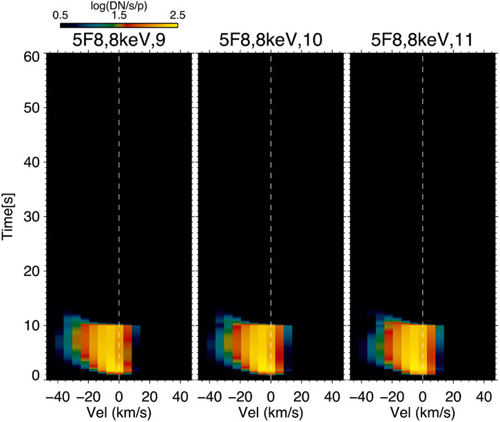
FIGURE A1. Time-velocity synthetic spectra of Si iv for RADYN flare simulations with initial apex temperature of 1 MK, F = 5F8, E_C = 8keV, and δ = 9,10 and 11. This image shows that different values of spectral index, within the constraints we obtained from NuSTAR, do not affect the results significantly.

FIGURE A2

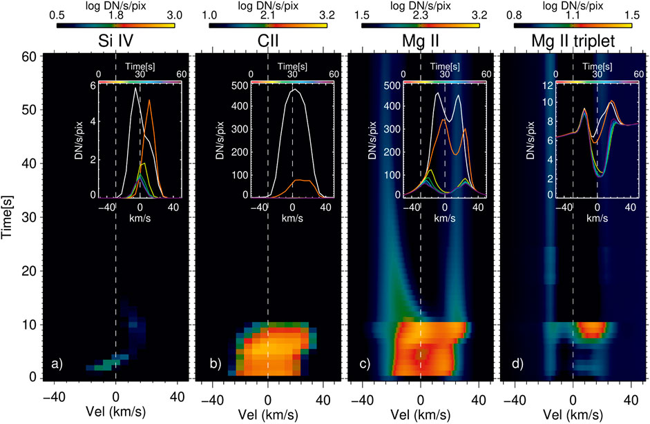
FIGURE A2. Top panels: Synthetic spectra from RADYN and RH simulations for the 1.2F9 flare model with E_C = 8 keV, δ = 10 and initial loop apex temperature of 3MK. The four panels show the: Si iv (Panel A), C ii (Panel B), Mg ii (Panel C) and Mg ii triplet (Panel D) lines as a function of velocity and time. The insert on each panel shows the spectra averaged in time with a cadence of 8s, as indicated by the legend.