SITCoM: SiRGraF Integrated Tool for Coronal dynaMics

1 Introduction

The white-light solar corona is associated with large-scale eruptions, coronal mass ejections (CMEs; Hundhausen et al., 1984; Gosling, 1993; Webb and Howard, 2012), reconnection-based plasmoids (Riley et al., 2007; Guo et al., 2013; Lee et al., 2020; Patel et al., 2020), coronal inflows (Wang et al., 1999; Sheeley and Wang, 2001; Sheeley and Wang, 2007; Sheeley and Wang, 2014; Hess and Wang, 2017), and streamer waves (Chen et al., 2010; Feng et al., 2013; Decraemer et al., 2020). All these phenomena are seen to exhibit a wide range of properties and are primarily observed and studied with white-light coronagraph imagery of the Large Angle Spectrometric Coronagraph (LASCO; Brueckner et al., 1995) of the Solar and Heliospheric Observatory (SOHO) and the Sun Earth Connection Coronal and Heliospheric Imager (SECCHI; Howard et al., 2008) onboard the Solar Terrestrial Relations Observatory (STEREO). It has been recently emphasized that most of the dynamics occur in the region from 1.5–6 R_⊙ defined as the middle corona (West et al., 2022). To capture such a wide variety of phenomena, it becomes important to separate these structures from the background and, at the same time, enhance their visibility in the coronagraph FOV of observation.

A couple of algorithms have been developed recently for white-light datasets to separate out the dynamic structures and reduce coronal intensity gradient. The normalizing radial gradient filter (NRGF; Morgan et al., 2006) and Simple Radial Gradient Filter (SiRGraF; Patel et al., 2022; Patel, 2022) are two such processing algorithms. Along similar lines, some algorithms have been used to enhance the off-limb structures in extreme ultraviolet images (Masson et al., 2014; Patel et al., 2021; Seaton et al., 2021; Seaton et al., 2023). In the manual CME detection catalog of the NASA Community Data Analysis Workshop (CDAW; Yashiro et al., 2004), CMEs can be tracked in their web interface by manually clicking the points in the running difference images. Automated CME detection has been performed with the aid of feature detection and image processing algorithms such as Computer Aided CME Tracking (CACTus; Robbrecht and Berghmans, 2004; Pant et al., 2016), the Solar Eruptive Events Detection System (SEEDS; Olmedo et al., 2008), Automatic Recognition of Transient Events and Marseille Inventory from Synoptic maps (ARTEMIS; Boursier et al., 2009), Coronal Image Processing (CORIMP; Byrne et al., 2012; Morgan et al., 2012), CMEs Identification in Inner Solar Corona (CIISCO; Patel et al., 2021), and algorithms based on machine learning (Qu et al., 2006; Zhang et al., 2017). These algorithms have been mainly designed for and applied on large-scale transients, but not on small-scale flows and blob-like structures.

Streamers are large-scale quasi-static bright structures and are seen to be stretched from the inner to outer corona in the eclipse images (Koutchmy and Livshits, 1992). CMEs are observed to displace streamers sideways and generate streamer oscillations (Chen et al., 2010; Feng et al., 2013; Kwon et al., 2013). The statistical study on streamer waves suggested that they can be a plausible candidate for coronal seismology (Decraemer et al., 2020). In the context of automatic detection of transverse oscillations in the solar corona, Northumbria University Wave Tracking (NUWT; Morton et al., 2016) was developed and extended by Weberg et al. (2018). The use of NUWT can be advantageous in carrying out statistical analysis of transverse waves. However, the NUWT code is best applicable for decayless waves observed in coronal loops (Weberg et al., 2018). Furthermore, the automatic identification and fitting of waves in time–distance (x − t) diagrams can be affected by the complex and varying backgrounds, as well as the presence of neighboring structures, which may necessitate manual fitting procedures. Additionally, there is a lack of a tool for quickly analyzing wave properties.

In recent times, JHelioviewer (Müller et al., 2017), an open-source data visualization tool was developed with basic image processing and integration of different catalogs for quick analysis before proceeding to an in-depth one. An automated data-mining-based web interface combined with feature detection has been developed as a part of the Heliophysics Events Knowledgebase (HEK; Hurlburt et al., 2012). Using the multi-instrument observations and tracking CMEs, solar energetic particles (SEPs), co-rotating interaction regions (CIRs), etc., a community-led effort by the European Space Agency’s Modelling and Data Analysis Working Group (MADAWG) developed several tools, e.g., the magnetic connectivity tool (Rouillard et al., 2020). Another web-based interface to track the CMEs, SEPs, and CIRs from the inner corona to the outer heliosphere is the “Propagation Tool” (Rouillard et al., 2017). Solar MAgnetic Connection Haus (SolarMACH; Gieseler et al., 2023), another open-source tool, was developed recently for the visualization of magnetic configurations and connections with various spacecraft and planetary bodies in the heliosphere. To track the CMEs based on multi-viewpoint observations from STEREO and SOHO coronagraphs, a web-based application called the STEREO CME Analysis Tool (StereoCAT; Millward et al., 2013) is hosted at the NASA Community Coordinated Modeling Center (https://ccmc.gsfc.nasa.gov/analysis/stereo/).

All these tools have been supported with basic image processing algorithms and are helpful in quick analysis serving their purposes. Often, the output of these tools has also been a part of in-depth scientific analysis. In this paper, we introduce an open-source tool, SiRGraF Integrated Tool for Coronal dynaMics (SITCoM), utilizing the SiRGraF algorithm and bringing out the dynamic features of the solar corona. This tool is currently targeted for studying the kinematics of CMEs, plasmoids, streamer blobs, outflows, inflows, etc., and the analysis of streamer waves and similar oscillatory phenomena. This paper is arranged as follows: In Section 2, we introduce and explain the architecture of the tool. The application of SITCoM for two broad aspects with illustrative examples is presented in Section 3 followed by a summary and discussion along with the scope of future improvements in Section 4.

2 Software design

sitcom is fully developed using Python and is temporarily made available as a PYPI package¹ and is mainly compiled using PyQt and has other small dependencies. It can be installed using the command pip install sitcom.

The software can be run for further use by the command in the terminal python3 -m sitcom.

Further updates will be released that will make it more flexible for different platforms. It is available on GitHub² as well for a better look at the code and to raise issues if any.

2.1 SiRGraF interface

The initial part of this graphical user interface (GUI) is shown in Figure 1 where the first step is the implementation of the SiRGraF algorithm. The interface is designed in such a way that the only task of the user is to provide the path containing FITS files in the given address bar by pasting a copied path or use the browse option available. The path for LASCO/C2 images for 07 January 2001 is shown for illustration. After providing the path of the data, the start button is used to initialize the process of implementation of SiRGraF and the status of which can be tracked in the status bar. Once the process is completed, the right panel in the GUI shows the minimum intensity, and uniform intensity images along with the average intensity profile and a sample filtered image after pressing the respective buttons are shown in Figure 1A. By default, linear intensity scaling is used to display all the generated image outputs.

FIGURE 1

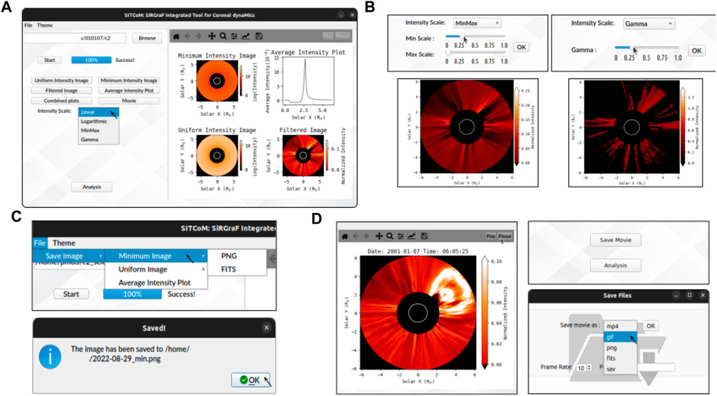
FIGURE 1. (A) An inclusive overview of the tools available in the SiRGraF part of the software including the availability to browse the path or add the path to data. (B) Intensity scaling options and the respective output below as applied on LASCO-C2 images. (C) Toolbar menu options to save images and to switch themes. On the bottom is the dialog box that appears when the “Minimum Image” is saved displaying the location of the saved file. (D). On the left is a screenshot of a paused frame of the movie, and on the right below are the available formats in which you may save the movie. The “Save movie” button appears when the “Movie” button is clicked.

The images filtered with SiRGraF can be visualized in an embedded matplotlib-based player consisting of basic functionalities such as Play, Pause, and Zoom in the toolbar; this, among other options to assess these images, will help in better evaluation of the data. This section also allows the user to perform the basic intensity scaling such as logarithmic, min–max, and gamma correction (Gonzalez and Woods, 2008). Figure 1B shows some of the different intensity scaling options available and the respective output when applied to SiRGRaF-processed LASCO/C2 images. Utilizing these options will help highlight certain features against others which can be used in the subsequent analysis section. In conjunction with that, the user can save individual elements of SiRGRaF such as the minimum and uniform images from the “File” option of the menu bar (Figure 1C). Additionally, the movie can be saved in “.mp4” and “.gif” (video formats) and “.png,” “.fits,” and “.sav” (saves each processed frame with the file name with the timestamp from the movie. For example, if the file name is “cme,” it will save files with one of the names as “cme-_MMDDTHHMMDD.png”). Along with this, an option to control the frame rate is also provided to save video formats. It creates a hierarchical structure of folders to save these files. For example, for a data file dated 6 July 2004, it will first create a folder named “2004-07-06” in the “/home/” directory and sub-folders within that “PNG,” “FITS,” and “SAV” depending on the chosen format to save. The movies will be saved in the “2004-07-06” folder.

An optional tool available in the menu bar is to switch the GUI theme to dark as it has lately become a preference of users worldwide. Once the feature of interest is identified, the user can proceed to the analysis section by using the “Analysis” button.

2.2 Analysis interface

An overview of the analysis using sitcom is presented through a flow chart in Figure 2. Upon clicking the “Analysis” button, a user is presented with options to estimate either the kinematic or oscillation properties of the dynamic event. The flow chart illustrates the series of processes that are executed when utilizing the application.

FIGURE 2

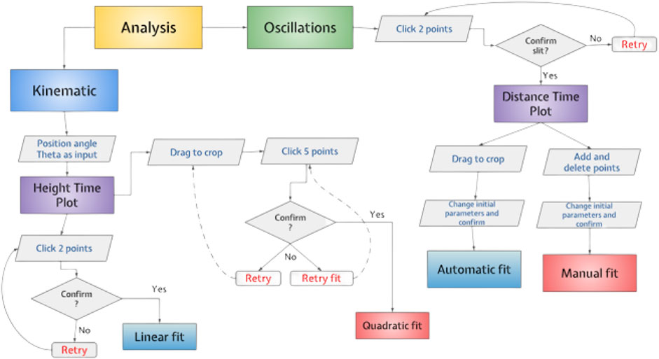
FIGURE 2. Mechanism of the analysis interface showing the steps required to obtain distance–time plots and consequently perform respective fits on them.

Figure 3 provides a snapshot of the GUI corresponding to the analysis interface. Clicking the analysis button takes the user to another window that is adjacent to the main interface. This section can also be accessed directly after the “Start” button has been clicked; i.e., this window contains two provisions that can be used for kinematics analysis and to carry out wave or oscillation studies.

FIGURE 3

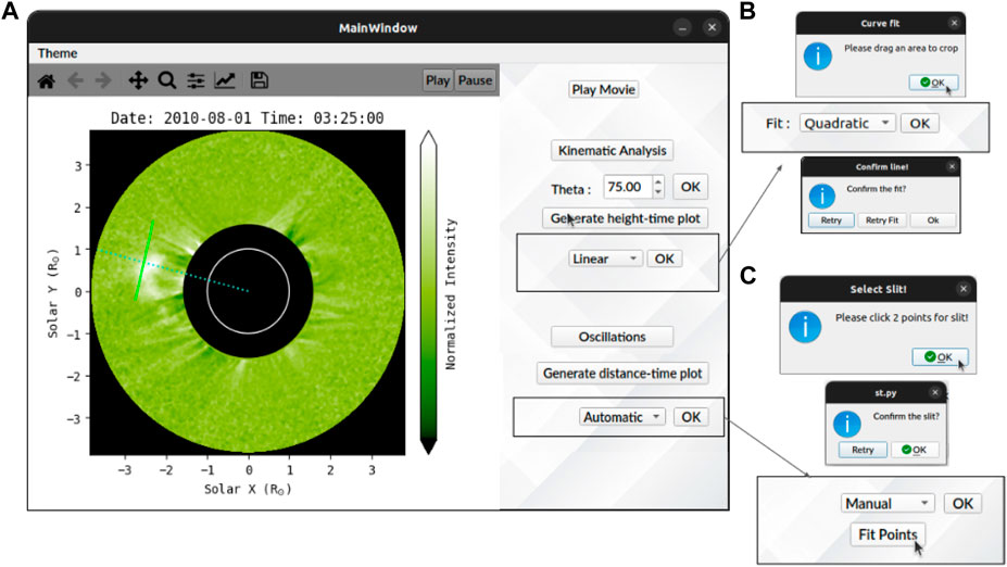
FIGURE 3. (A) An overview of the analysis interface showing the PA with a dotted line and selected slit with a solid green line. (B) Dialog boxes that pop up when performing a quadratic fit. (C) Option to select slit after the user presses the “Oscillations” button. The fitting can be performed manually or using automatic fit selection.

The kinematic analysis section allows the user to generate height–time plots at various position angles and perform linear or higher-order fitting on selected data points. The fittings provide information about the velocity and acceleration of the feature, depending on the type of fitting used. The “Retry” option is available to help obtain better-fit values if required. Additionally, the option for linear fitting is selected by default and can be updated through a drop-down menu. To perform a linear fit, the user can first use the toolbar zoom and then click two points (Section 3.1.1). As shown in 3B, for quadratic fitting, the user is required to first drag an area to zoom in and then click five points for fitting. Two retry options are available: clicking the “Retry” button plots the original height–time graph, allowing the user to zoom again on a different region by dragging a rectangle, while clicking “Retry Fit” clears the currently fitted points, enabling the user to perform the fit again for the already zoomed region. These options can be availed as many times as needed. After the fit is satisfactory, it can be confirmed by “Ok,” and a plot with velocity and/or acceleration obtained from the fit will be displayed.

Another option is to analyze oscillations by placing an artificial slit across a feature, which generates a distance–time plot over the length of the slit. The “Oscillation” tab on the interface allows users to choose an artificial slit of their desired position by clicking two points in the movie frame. Once the slit is selected, a dialog box will pop up to confirm the selection. If the user wants to reselect the slit, they can use the “Retry” option on the pop-up box (Figure 3C). After selecting the slit, the user can produce distance-time (x − t) maps by clicking on the option “Generate distance–time plot,” with “Automatic fit” set as the default option. If there are any oscillations in the x − t map, the user can fit these oscillations by selecting the region using drag crop around the oscillation (for automatic fit) or the toolbar zoom option (for manual fit) and then perform fit through a series of steps. This fitting procedure is discussed in Section 3.2.1 with examples.

3 Data used and software functionality

We acquired the level 0.5 data of the C2 coronagraph of LASCO from the Virtual Solar Observatory (VSO) for 29 August 2022. We converted the data into level 1 using the reduce_level_1.pro procedure available in the solar software (SSW) to correct for the image rotation and calibration. Other LASCO/C2 data presented in this paper were already level 1 corrected. Apart from these, STEREO/COR-1 data have also been used. Level 0.5 polarized brightness triplets (0°, 120°, 240°) of COR-1 are acquired from VSO for the date of 1 August 2010. These images are reduced to level 1 using the secchi_prep.pro procedure of the STEREO pipeline. The triplets are combined to obtain the total brightness images which are also calibrated and rotation corrected in this step. The level 1 data of LASCO/C2 and COR-1 are provided to the SITCoM analysis tool as FITS files.

3.1 Kinematics of transients

3.1.1 CME case

CMEs are identified as propagating white-light large-scale structures in the coronagraph field of view (FOV) (Hundhausen et al., 1984). An application is illustrated in Figure 4 with the LASCO/C2 dataset of 07 January 2001, where a CME occurred at the northwest limb of the Sun. This CME has also been shown as a representative example for demonstrating the NRGF by Morgan et al. (2006) and the SiRGraF by Patel et al. (2022). It is known that CMEs, after reaching heights beyond ∼3 R_⊙, attain a constant speed (Majumdar et al., 2020). This height also lies in the middle corona within the LASCO field of view, and hence, CMEs can be considered to have a linear profile in the height–time plot. As shown in Figure 4, any position angle can be provided to generate the height–time plot; for this case, we have used a PA of 298°. Once it is generated, the bright ridge corresponding to the CME can be zoomed in using the toolbar zoom icon, and the leading edge can be fitted with a straight line by clicking two points (after de-selecting the zoom icon). The interface provides an option to retry and finalize the points for the fit, to confirm it. Once confirmed, a plot with the value for the velocity of the CME will be displayed. For the example presented here, the speed estimated here of 588 km·s⁻¹ matches well with the value in the CDAW catalog as 633 km·s⁻¹.

FIGURE 4

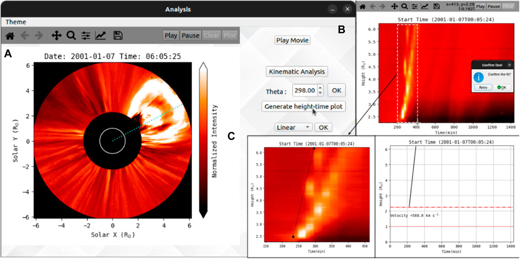
FIGURE 4. (A) Movie frame showing a dashed line at the PA of 298°. (B) Usage of the zoom tool to crop the region for fitting on the height–time plot. (C) Linear fit confirmed after clicking two points showing a velocity of 588 km·s⁻¹.

Most of the CMEs which are observed in STEREO/COR-1 are still undergoing an acceleration phase. This is also seen in an example shown in Figure 5 where a CME was observed in COR-1B on 01 August 2010, at the northeast limb. The height–time plot is generated along the dotted green line shown in the coronagraph image and is shown in the (b) panel of the same figure. The leading edge of the CME is seen with a curved profile suggesting the presence of acceleration. Using the available quadratic fit option, data points are selected in the height–time plot. The points are confirmed for fit by visual inspection. We found that this CME showed an acceleration of ≈156 m·s⁻² in the COR-1B FOV and an average speed of 249 km·s⁻¹.

FIGURE 5

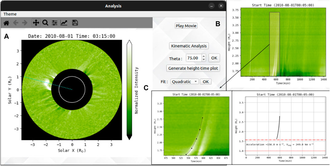
FIGURE 5. (A) Movie frame showing a line at the PA of 75°. (B) Usage of the drag rectangle to crop the region for fitting on the height–time plot. (C) Quadratic fit confirmed after clicking five points showing the values of acceleration and average velocity.

3.1.2 Plasma blobs case

Plasma blobs arising due to magnetic reconnection have been considered as one of the transient structures formed in the Sun’s corona. These may be associated with CMEs often observed in coronagraph images post-CME rays (Webb and Vourlidas, 2016) and the streamer blobs originating at the tip of streamers. These blobs appear as small-scale discrete white-light structures with nearly elliptical shapes in coronagraph images. Figure 6 shows one of the many plasma blobs observed along the post-CME current sheet on 10 September 2017. The right panel of the figure shows the distance–time plot generated for the position angle of 262°. The first ridge corresponds to the leading edge of the CME followed by plasma blobs. It can be noticed in the distance–time plot that the observed blobs show inclined ridges; hence, we used linear fitting to characterize the speed. The velocity of the blob is displayed after confirming the plot fit. The estimated speed of ≈1,000 km·s⁻¹ agrees with the speed distribution of plasma blobs observed in LASCO/C2 FOV for this dataset reported by Patel et al. (2020). The distance–time plot also reveals more ridges following the one used for analysis. These correspond to the successive blobs which can be approached in a similar way to measure their speeds.

FIGURE 6

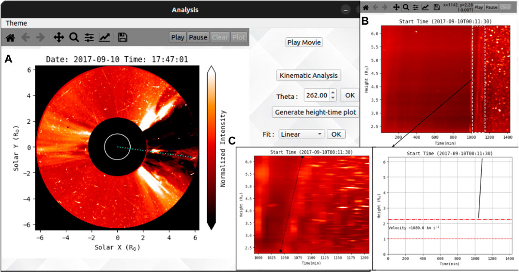
FIGURE 6. (A) Movie frame with the dotted line at the PA of 262° along the plasma blob. (B) Usage of the zoom tool to crop the region for fitting on the height–time plot. (C) Linear fit on the ridge of the plasma blob, showing a velocity of 1,089 km·s⁻¹.

3.1.3 Inflow case

Often, material has been observed falling toward the Sun after a CME has passed in the LASCO FOV. This in-falling material can be seen as a result of partial eruption or dark inflows which are in the wake of the CME. These structures have been tracked manually in many studies in the past. The SITCoM interface has been tested to track such features using LASCO/C2 images. An example of dark inflow is shown in Figure 7 where these flows are observed on 12 October 2005, moving toward the Sun after the CME has passed in LASCO FOV. The dotted line represents the position angle of 221° used to track the inflow. The height–time plot is generated corresponding to this dotted line and is shown in Figure 7B. The color map of this plot is inverted for the visualization of the ridge corresponding to the inflow. This ridge shows straight-line behavior, and therefore, linear fitting was used to estimate its speed. The fitted curve is shown in panel (c). The negative value of the measured speed indicates that the structure is moving toward the Sun. In case curved ridges are observed for the sunward moving material, as in the studies such as Tripathi et al. (2007) and Longcope et al. (2018), then quadratic fit can be used to measure the kinematics of such flows.

FIGURE 7

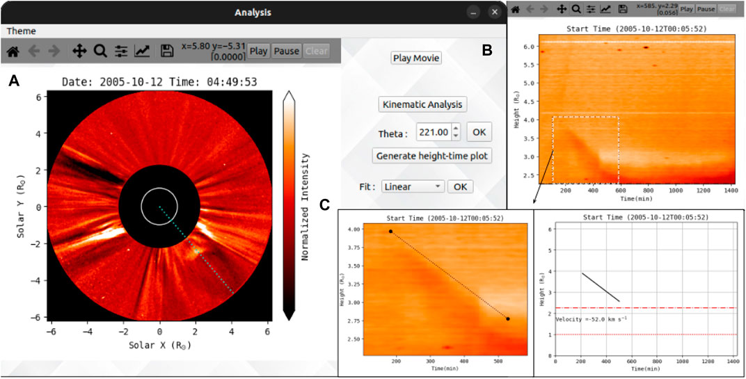
FIGURE 7. (A) The dark curve as seen in the movie frame along the PA of 221° is the observed inflow in LASCO FOV. (B) Usage of the zoom tool to crop the region of the dark ridge. (C) Linear fit performed on the inner edge, showing a velocity of −52 km·s⁻¹, indicating in-flowing material.

3.2 Oscillations and waves

3.2.1 Streamer wave case

To demonstrate the analysis of oscillations in helmet streamers perturbed by CMEs, we present two case studies. In this section, we outline the methodology used, involving the SiRGraF algorithm as described in Section 2.1, and highlight the analysis tool employed for accurate data interpretation. By choosing the “Play Movie” option in the interface (Figure 3A), users can access a movie displaying the SiRGraF-processed images. This feature assists in identifying the optimal placement for the artificial slit, by clicking two points on the frame, corresponding to the desired location. The interface allows for multiple retries, ensuring the selection of the most appropriate slit placement.

3.2.2 Manual fitting

We use the set of LASCO/C2 level-1 images of 29 August 2022 between 15:12 and 23:48 UT for the illustration of the manual fitting case, where a CME was observed near the western limb, perturbing the streamer as it propagated in the radial direction. We selected the slit perpendicular to the streamer (Figure 8A). The “Generate distance–time plot” button on the interface collates the intensities at the slit position for every frame and produces an x − t map. While still under development, the features provided in manual fitting are to perform fit on the distance–time plot through a series of simple steps implemented in the current version.

1. Click on the zoom icon and crop the region of interest.

2. Deselect the zoom icon and use the left-click button to add a point where the mouse pointer is. The right-click button deletes the last added point (Figure 8B).

3. Once the points are ready for fit, click on the “Fit Points” button (Figures 8C–D), which will open a window displaying the parameters of the current fit and will fit the current points based on this initial guess. The profile of selected points will be fitted using a decaying sinusoidal function of the following form (Nakariakov et al., 1999):

$y\left(x\right)=p_0+p_1\sin \left(\frac{2\pi x}{p_2}+p_3\right)e^{\frac{-x}{p_4}}+p_{5}x,(1)$

where p₀ is the mean position, p₁ is the initial amplitude of the oscillation, p₂ is the period of oscillation, p₃ denotes the phase, p₄ indicates the damping time, and p₅ is the coefficient for the linear trend.

4. These parameters can be updated or changed to modify the fit according to the needs of the user to attain a better fit.

5. After that, the “Plot” button can be clicked to generate the final curve used for fit, and their respective parameter will be automatically saved into a “.csv” file in the “/home/” directory.

FIGURE 8

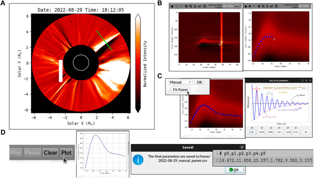
FIGURE 8. (A) Selected slit on the movie frame from LASCO C2 data of 29 August 2022, perpendicular to the streamer. (B) Required area to fit on the generated distance–time plot is first zoomed on, and then, points are selected for fit. (C) “Fit Points” button performs a fit on the current points based on the initial guess and pops open a window to modify parameters for this fit. (D) Next, this fit is plotted and parameters are saved in a “.csv” file as shown in the dialog box; the movie is available in the online version.

The user can click on the “Generate distance–time plot” button as many times as required to retry the fit from the beginning. For this particular case of the streamer, we got the initial perturbation amplitude, period, and damping time as 0.14 R_⊙, 253 min, and 96 min, respectively, which are consistent with previous streamer wave events depicted in the work of Chen et al. (2010), Kwon et al. (2013), and Decraemer et al., 2020. The period and damping time relation at different heliocentric distances can be used to check the wave mode of the streamer wave (Ofman and Aschwanden, 2002).

3.2.3 Automatic fitting

We use LASCO/C2 level 1 images of 06 July 2004 between 00:04 and 23:52 UT for the illustration of the automatic fitting case. A streamer is perturbed by a CME located near the southwest region in the LASCO image (see Figure 9). We selected the slit perpendicular to the streamer and used the “Generate distance-time plot” to produce an x − t map. As shown in the figure, after the plot is generated, the user can select the constricted part where the oscillation occurs by dragging a rectangle around that region. At every time step (corresponding to columns in the x − t map), a Gaussian profile is fitted across the slit length to find out the position of the oscillating streamer. An initial automatic fit, based on Eq. 1, will be performed on that region (note: the user may have to try for different rectangles around the oscillation for better fit). This part can be retried many times by clicking on the “Generate distance–time plot” button. After the fit is performed with the initial guess, another window shows up with these parameters (similar to manual fitting), which can be modified to improve the fit. The automatic fit can be advantageous over manual fit as it can remove the human bias created by selecting the points on the x–t map. We found the initial amplitude, period, and damping time from the automatic fit as 0.2 R_⊙, 95 min, and 88 min, respectively. Using a sample of 22 events, Decraemer et al. (2020) determined the average period of streamer waves as 239 min; a similar order of magnitude values are obtained using manual and automatic fit techniques in this work. The period determination could be further used to calculate phase speed and an estimate of background solar wind speed considering the wavelength is known (Decraemer et al., 2020). The measurement of phase speed could also be useful in determining the magnetic fields in the streamers (Chen et al., 2011). In brief, SITCoM is a useful tool for quickly analyzing the oscillation properties of streamer waves.

FIGURE 9

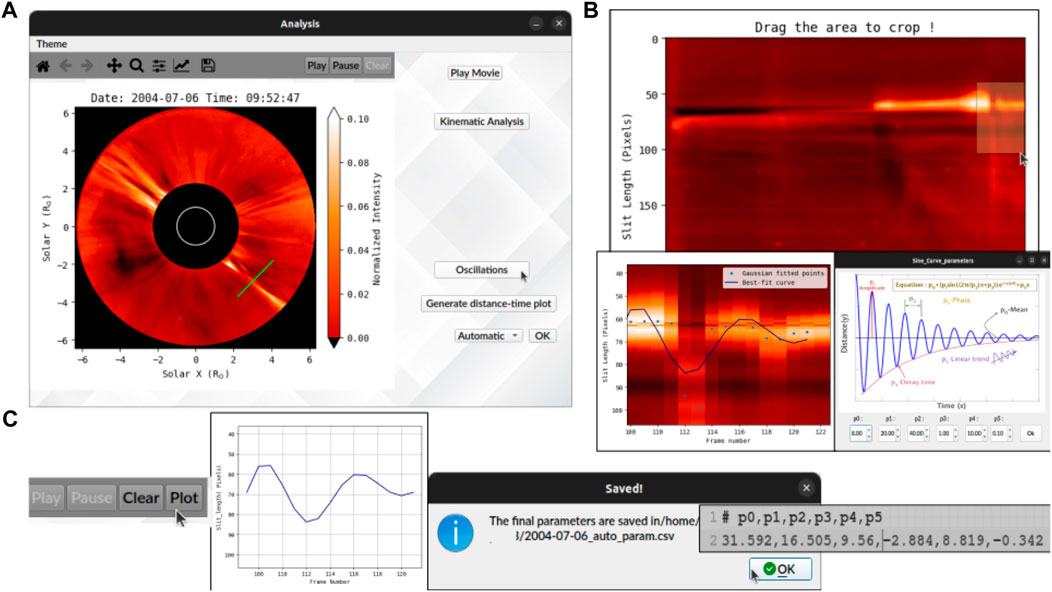
FIGURE 9. (A) Selected slit on the movie frame from LASCO C2 data of 06 July 2004, perpendicular to the streamer. (B) Selected area on the generated distance–time plot, showing oscillations, is first zoomed on, and then, the automatic fitting is performed with an initial guess. (C) After plotting the final fit, the parameters of the fit will be saved in a “.csv” file.

4 Summary and future developments

We introduce a new tool, SITCoM, which is built upon the SiRGRaF algorithm for processing white-light coronagraph images. The application enables rapid analysis of coronal dynamics such as CMEs, plasma blobs, streamer waves, and similar transients, observed in white-light coronagraph data. The output of SITCoM can serve as preliminary analysis for in-depth scientific investigations or can be integrated into larger studies using various datasets. SITCoM is developed as an open-source application that features a simple user interface based on PyQT and other minor dependencies in Python. It can be installed using the pip command in Python.

The SITCoM GUI incorporates the SiRGRaF algorithm in its initial stage, which proves to be a simple yet effective tool for highlighting dynamic features in the corona. The dynamic features are enhanced against the background throughout the coronagraph FOV. We illustrated the usage of SITCoM using LASCO and STEREO or white-light coronagraph data for various test cases. Since SiRGRaF has also been implemented on Solar Orbiter Metis data by Telloni et al. (2022), it can be used in the SITCoM as input along with the aforementioned datasets. Along with these datasets, the application of SiRGraF on the extreme ultraviolet (EUV) dataset will require detailed analysis and testing including image processing to enhance the structures observed in EUV passbands. The future updates of SITCoM will be equipped with such image-enhancing features to carry out the analysis presented here. Users have the capability to save the processed movie and individual frames in various formats. Moreover, SITCoM offers different intensity scaling, such as MinMax, Logarithmic, and Gamma, allowing users to enhance specific features based on their preferences and requirements.

To facilitate kinematics analysis of any sunward or anti-sunward moving structures in the data, SITCoM empowers users to generate height–time plots at different position angles. These plots provide valuable insights into the temporal evolution of the observed phenomena. The users can perform linear or higher-order fitting on these plots to derive essential parameters such as velocity or acceleration, depending on the type of fitting performed. Multiple measurements can be made at the same position angle or over desired angles to get an estimate of deviation in the measured kinematics throughout the large-scale structures.

Users can also investigate various types of oscillations and waves within a selected slit across a dynamic feature. By employing a decaying sine wave-fitting technique, users can automatically or manually fit the resultant distance–time plot generated from the slit. The extracted parameters of the fitted wave can be saved for further analysis, providing insights into the oscillatory behavior of coronal features.

This GUI is not only a powerful tool for analyzing coronal dynamics but also saves time typically spent on plotting and fitting. By streamlining the analysis process, SITCoM provides useful results obtained with quick analysis. The combination of advanced algorithms and user-friendly tools facilitates a comprehensive understanding of the observed phenomena, enhancing our knowledge in this field. In the future, we plan to develop SITCoM for different platforms to make it more accessible to researchers worldwide. This will enable more scientists to benefit from its capabilities and contribute to our understanding of the Sun’s corona.

We plan to improve the SITCoM application with the addition of new features in the future. These include the implementation of fitting multiple ridges identified in the height–time plots for kinematics analysis. As a result, multiple transients at the same position angle can be tracked and characterized manually without having to generate the same x–t map repeatedly. Implementation of curved slit selection will enable a user to select a curved slit for the generation of x–t maps. Such a feature will be helpful to characterize the CME deflection and non-radial flows (Alzate et al., 2023) as well as tracking the waves and oscillations at bigger regions of interest using a single large slit or a wide slit. A provision to save the coordinates corresponding to the slit location and the x–t map array in the form of FITS or “.sav” file will be useful to revisit an analysis later or import to any other program when required.

These planned advancements will further enhance the capability of SITCoM and will be a part of its future releases.

Data availability statement

The datasets presented in this study can be found in online repositories. The names of the repository/repositories and accession number(s) can be found at: https://github.com/pu3/SITCoM.

Author contributions

RP planned the development and overlooked the implementation of the tool. PU and AS developed the tool in Python and carried out tests on different datasets. PU and AS prepared the manuscript. All authors contributed to the article and approved the submitted version.

Funding

AS was supported by the Council of Scientific and Industrial Research (CSIR), India, under file no. 09/079(2872)/2021-EMR-I.

Acknowledgments

PU and AS would like to thank ARIES for providing the computational facilities. The SECCHI data used here were produced by an international consortium of the Naval Research Laboratory (United States), the Lockheed Martin Solar and Astrophysics Lab (United States), the NASA Goddard Space Flight Center (United States), the Rutherford Appleton Laboratory (United Kingdom), the University of Birmingham (United Kingdom), the Max Planck Institute for Solar System Research (Germany), Centre Spatiale de Li$\grave{e}$ge (Belgium), Institut d’Optique Th$\acute{e}$orique et Appliqu$\acute{e}$e (France), and Institut d’Astrophysique Spatiale (France). The authors also thank NASA for making SOHO/LASCO data publicly available.

Conflict of interest

The authors declare that the research was conducted in the absence of any commercial or financial relationships that could be construed as a potential conflict of interest.

Publisher’s note

All claims expressed in this article are solely those of the authors and do not necessarily represent those of their affiliated organizations, or those of the publisher, the editors, and the reviewers. Any product that may be evaluated in this article, or claim that may be made by its manufacturer, is not guaranteed or endorsed by the publisher.

Supplementary material

The Supplementary Material for this article can be found online at: https://www.frontiersin.org/articles/10.3389/fspas.2023.1227872/full#supplementary-material

Footnotes

¹PYPI: https://pypi.org/project/sitcom/

²GitHub: https://github.com/pu3/SITCoM

References

Alzate, N., Morgan, H., and Di Matteo, S. (2023). Tracking nonradial outflows in extreme ultraviolet and white light solar images. Astrophys. J. 945, 116. doi:10.3847/1538-4357/acba08

CrossRef Full Text | Google Scholar

Boursier, Y., Lamy, P., Llebaria, A., Goudail, F., and Robelus, S. (2009). The ARTEMIS catalog of LASCO coronal mass ejections: automatic recognition of transient events and Marseille inventory from synoptic maps. Sol. Phys. 257, 125–147. doi:10.1007/s11207-009-9370-5

CrossRef Full Text | Google Scholar

Brueckner, G. E., Howard, R. A., Koomen, M. J., Korendyke, C. M., Michels, D. J., Moses, J. D., et al. (1995). The large angle spectroscopic coronagraph (LASCO). Sol. Phys. 162, 357–402. doi:10.1007/BF00733434

CrossRef Full Text | Google Scholar

Byrne, J. P., Morgan, H., Habbal, S. R., and Gallagher, P. T. (2012). Automatic detection and tracking of coronal mass ejections. II. Multiscale filtering of coronagraph images. Astrophys. J. 752, 145. doi:10.1088/0004-637X/752/2/145

CrossRef Full Text | Google Scholar

Chen, Y., Feng, S. W., Li, B., Song, H. Q., Xia, L. D., Kong, X. L., et al. (2011). A coronal seismological study with streamer waves. Astrophys. J. 728, 147. doi:10.1088/0004-637X/728/2/147

CrossRef Full Text | Google Scholar

Chen, Y., Song, H. Q., Li, B., Xia, L. D., Wu, Z., Fu, H., et al. (2010). Streamer waves driven by coronal mass ejections. Astrophys. J. 714, 644–651. doi:10.1088/0004-637X/714/1/644

CrossRef Full Text | Google Scholar

Decraemer, B., Zhukov, A. N., and Van Doorsselaere, T. (2020). Properties of streamer wave events observed during the STEREO era. Astrophys. J. 893, 78. doi:10.3847/1538-4357/ab8194

CrossRef Full Text | Google Scholar

Feng, L., Inhester, B., and Gan, W. Q. (2013). Kelvin-helmholtz instability of a coronal streamer. Astrophys. J. 774, 141. doi:10.1088/0004-637X/774/2/141

CrossRef Full Text | Google Scholar

Gieseler, J., Dresing, N., Palmroos, C., Freiherr von Forstner, J. L., Price, D. J., Vainio, R., et al. (2023). Solar-MACH: an open-source tool to analyze solar magnetic connection configurations. Front. Astronomy Space Sci. 9, 384. doi:10.3389/fspas.2022.1058810

CrossRef Full Text | Google Scholar

Gonzalez, R. C., and Woods, R. E. (2008). Digital image processing. Upper Saddle River, N.J. Prentice Hall.

Google Scholar

Gosling, J. T. (1993). The solar flare myth. J. Geophys. Res. 98, 18937–18949. doi:10.1029/93JA01896

CrossRef Full Text | Google Scholar

Guo, L. J., Bhattacharjee, A., and Huang, Y. M. (2013). Distribution of plasmoids in post-coronal mass ejection current sheets. Astrophys. J. Lett. 771, L14. doi:10.1088/2041-8205/771/1/L14

CrossRef Full Text | Google Scholar

Hess, P., and Wang, Y. M. (2017). Inflows in the inner white-light corona: the closing-down of flux after coronal mass ejections. Astrophys. J. 850, 6. doi:10.3847/1538-4357/aa921d

CrossRef Full Text | Google Scholar

Howard, R. A., Moses, J. D., Vourlidas, A., Newmark, J. S., Socker, D. G., Plunkett, S. P., et al. (2008). Sun Earth connection coronal and heliospheric investigation (SECCHI). Space Sci. Rev. 136, 67–115. doi:10.1007/s11214-008-9341-4

CrossRef Full Text | Google Scholar

Hundhausen, A. J., Sawyer, C. B., House, L., Illing, R. M. E., and Wagner, W. J. (1984). Coronal mass ejections observed during the solar maximum mission - latitude distribution and rate of occurrence. J. Geophys. Res. 89, 2639–2646. doi:10.1029/ja089ia05p02639

CrossRef Full Text | Google Scholar

Hurlburt, N., Cheung, M., Schrijver, C., Chang, L., Freeland, S., Green, S., et al. (2012). Heliophysics event Knowledgebase for the solar dynamics observatory (SDO) and beyond. Sol. Phys. 275, 67–78. doi:10.1007/s11207-010-9624-2

CrossRef Full Text | Google Scholar

Koutchmy, S., and Livshits, M. (1992). Coronal streamers. Space Sci. Rev. 61, 393–417. doi:10.1007/BF00222313

CrossRef Full Text | Google Scholar

Kwon, R. Y., Ofman, L., Olmedo, O., Kramar, M., Davila, J. M., Thompson, B. J., et al. (2013). STEREO observations of fast magnetosonic waves in the extended solar corona associated with EIT/EUV waves. Astrophys. J. 766, 55. doi:10.1088/0004-637X/766/1/55

CrossRef Full Text | Google Scholar

Lee, J. O., Cho, K. S., Lee, K. S., Cho, I. H., Lee, J., Miyashita, Y., et al. (2020). Formation of post-CME blobs observed by LASCO-C2 and K-cor on 2017 september 10. Astrophys. J. 892, 129. doi:10.3847/1538-4357/ab799a

CrossRef Full Text | Google Scholar

Longcope, D., Unverferth, J., Klein, C., McCarthy, M., and Priest, E. (2018). Evidence for downflows in the narrow plasma sheet of 2017 september 10 and their significance for flare reconnection. Astrophys. J. 868, 148. doi:10.3847/1538-4357/aaeac4

CrossRef Full Text | Google Scholar

Majumdar, S., Pant, V., Patel, R., and Banerjee, D. (2020). Connecting 3D evolution of coronal mass ejections to their source regions. Astrophys. J. 899, 6. doi:10.3847/1538-4357/aba1f2

CrossRef Full Text | Google Scholar

Masson, S., McCauley, P., Golub, L., Reeves, K. K., and DeLuca, E. E. (2014). Dynamics of the transition corona. Astrophys. J. 787, 145. doi:10.1088/0004-637X/787/2/145

CrossRef Full Text | Google Scholar

Millward, G., Biesecker, D., Pizzo, V., and de Koning, C. A. (2013). An operational software tool for the analysis of coronagraph images: determining CME parameters for input into the WSA-enlil heliospheric model. Space weather. 11, 57–68. doi:10.1002/swe.20024

CrossRef Full Text | Google Scholar

Morgan, H., Byrne, J. P., and Habbal, S. R. (2012). Automatically detecting and tracking coronal mass ejections. I. Separation of dynamic and quiescent components in coronagraph images. Astrophysical J. 752, 144. doi:10.1088/0004-637x/752/2/144

CrossRef Full Text | Google Scholar

Morgan, H., Habbal, S. R., and Woo, R. (2006). The depiction of coronal structure in white-light images. Sol. Phys. 236, 263–272. doi:10.1007/s11207-006-0113-6

CrossRef Full Text | Google Scholar

Morton, R. J., Mooroogen, K., and McLaughlin, J. A. (2016). Nuwt: Northumbria university wave tracking (nuwt) code. Zenodo.

Google Scholar

Müller, D., Nicula, B., Felix, S., Verstringe, F., Bourgoignie, B., Csillaghy, A., et al. (2017). JHelioviewer. Time-dependent 3D visualisation of solar and heliospheric data. Astron. Astrophys. 606, A10. doi:10.1051/0004-6361/201730893

CrossRef Full Text | Google Scholar

Nakariakov, V. M., Ofman, L., Deluca, E. E., Roberts, B., and Davila, J. M. (1999). TRACE observation of damped coronal loop oscillations: implications for coronal heating. Science 285, 862–864. doi:10.1126/science.285.5429.862

PubMed Abstract | CrossRef Full Text | Google Scholar

Ofman, L., and Aschwanden, M. J. (2002). Damping time scaling of coronal loop oscillations deduced from [ITAL]transition region and coronal explorer[/ITAL] observations. Astrophys. J. Lett. 576, L153–L156. doi:10.1086/343886

CrossRef Full Text | Google Scholar

Olmedo, O., Zhang, J., Wechsler, H., Poland, A., and Borne, K. (2008). Automatic detection and tracking of coronal mass ejections in coronagraph time series. Sol. Phys. 248, 485–499. doi:10.1007/s11207-007-9104-5

CrossRef Full Text | Google Scholar

Pant, V., Willems, S., Rodriguez, L., Mierla, M., Banerjee, D., and Davies, J. A. (2016). Automated detection of coronal mass ejections in STEREO heliospheric imager data. Astrophys. J. 833, 80. doi:10.3847/1538-4357/833/1/80

CrossRef Full Text | Google Scholar

Patel, R. (2022). Characterizing solar eruptions in inner corona using ground and space-based data. Ph.D. thesis. ARIES, Nainital.

Google Scholar

Patel, R., Majumdar, S., Pant, V., and Banerjee, D. (2022). A simple radial gradient filter for batch-processing of coronagraph images. Sol. Phys. 297, 27. doi:10.1007/s11207-022-01957-y

CrossRef Full Text | Google Scholar

Patel, R., Pant, V., Chandrashekhar, K., and Banerjee, D. (2020). A statistical study of plasmoids associated with a post-CME current sheet. Astron. Astrophys. 644, A158. doi:10.1051/0004-6361/202039000

CrossRef Full Text | Google Scholar

Patel, R., Pant, V., Iyer, P., Banerjee, D., Mierla, M., and West, M. J. (2021). Automated detection of accelerating solar eruptions using parabolic hough transform. Sol. Phys. 296, 31. doi:10.1007/s11207-021-01770-z

CrossRef Full Text | Google Scholar

Qu, M., Shih, F. Y., Jing, J., and Wang, H. (2006). Automatic detection and classification of coronal mass ejections. Sol. Phys. 237, 419–431. doi:10.1007/s11207-006-0114-5

CrossRef Full Text | Google Scholar

Riley, P., Lionello, R., Mikić, Z., Linker, J., Clark, E., Lin, J., et al. (2007). Bursty reconnection following solar eruptions: MHD simulations and comparison with observations. Astrophys. J. 655, 591–597. doi:10.1086/509913

CrossRef Full Text | Google Scholar

Robbrecht, E., and Berghmans, D. (2004). Automated recognition of coronal mass ejections (CMEs) in near-real-time data. Astron. Astrophys. 425, 1097–1106. doi:10.1051/0004-6361:20041302

CrossRef Full Text | Google Scholar

Rouillard, A. P., Lavraud, B., Génot, V., Bouchemit, M., Dufourg, N., Plotnikov, I., et al. (2017). A propagation tool to connect remote-sensing observations with in-situ measurements of heliospheric structures. Planet. Space Sci. 147, 61–77. doi:10.1016/j.pss.2017.07.001

CrossRef Full Text | Google Scholar

Rouillard, A. P., Pinto, R. F., Vourlidas, A., De Groof, A., Thompson, W. T., Bemporad, A., et al. (2020). Models and data analysis tools for the Solar Orbiter mission. Astron. Astrophys. 642, A2. doi:10.1051/0004-6361/201935305

CrossRef Full Text | Google Scholar

Seaton, D. B., Berghmans, D., De Groof, A., D’Huys, E., Nicula, B., Rachmeler, L. A., et al. (2023). The SWAP filter: A simple azimuthally-varying radial filter for wide-field EUV solar images. arXiv.

CrossRef Full Text | Google Scholar

Seaton, D. B., Hughes, J. M., Tadikonda, S. K., Caspi, A., DeForest, C. E., Krimchansky, A., et al. (2021). The Sun’s dynamic extended corona observed in extreme ultraviolet. Nat. Astron. 5, 1029–1035. doi:10.1038/s41550-021-01427-8

CrossRef Full Text | Google Scholar

Sheeley, J., and Wang, Y. M. (2014). Coronal inflows during the interval 1996-2014. Astrophys. J. 797, 10. doi:10.1088/0004-637X/797/1/10

CrossRef Full Text | Google Scholar

Sheeley, J., and Wang, Y. M. (2001). Coronal inflows and sector magnetism. Astrophys. J. Lett. 562, L107–L110. doi:10.1086/338104

CrossRef Full Text | Google Scholar

Sheeley, J., and Wang, Y. M. (2007). Out pairs and the detachment of coronal streamers. Astrophys. J. 655, 1142–1156. doi:10.1086/510323

CrossRef Full Text | Google Scholar

Telloni, D., Zank, G. P., Stangalini, M., Downs, C., Liang, H., Nakanotani, M., et al. (2022). Observation of a magnetic switchback in the solar corona. Astrophysical J. Lett. 936, L25. doi:10.3847/2041-8213/ac8104

CrossRef Full Text | Google Scholar

Tripathi, D., Solanki, S. K., Mason, H. E., and Webb, D. F. (2007). A bright coronal downflow seen in multi-wavelength observations: evidence of a bifurcating flux-rope? Astron. Astrophys. 472, 633–642. doi:10.1051/0004-6361:20077707

CrossRef Full Text | Google Scholar

Wang, Y. M., Sheeley, J., Howard, R. A., Cyr, O. C. S., and Simnett, G. M. (1999). Coronagraph observations of inflows during high solar activity. Geophys. Res. Lett. 26, 1203–1206. doi:10.1029/1999GL900209

CrossRef Full Text | Google Scholar

Webb, D. F., and Howard, T. A. (2012). Coronal mass ejections: observations. Living Rev. Sol. Phys. 9, 3. doi:10.12942/lrsp-2012-3

CrossRef Full Text | Google Scholar

Webb, D. F., and Vourlidas, A. (2016). LASCO white-light observations of eruptive current sheets trailing CMEs. Sol. Phys. 291, 3725–3749. doi:10.1007/s11207-016-0988-9

CrossRef Full Text | Google Scholar

Weberg, M. J., Morton, R. J., and McLaughlin, J. A. (2018). An automated algorithm for identifying and tracking transverse waves in solar images. Astrophys. J. 852, 57. doi:10.3847/1538-4357/aa9e4a

CrossRef Full Text | Google Scholar

West, M. J., Seaton, D. B., Wexler, D. B., Raymond, J. C., Del Zanna, G., Rivera, Y. J., et al. (2022). Defining the middle corona. arXiv.

Google Scholar

Yashiro, S., Gopalswamy, N., Michalek, G., Cyr, St.O. C., Plunkett, S. P., Rich, N. B., et al. (2004). A catalog of white light coronal mass ejections observed by the SOHO spacecraft. J. Geophys. Res. (Space Phys. 109, A07105. doi:10.1029/2003JA010282

CrossRef Full Text | Google Scholar

Zhang, L., Yin, J. Q., Lin, J. B., Feng, Z. Q., and Zhou, J. (2017). Detection of coronal mass ejections using multiple features and space–time continuity. Sol. Phys. 292, 91. doi:10.1007/s11207-017-1107-2

CrossRef Full Text | Google Scholar