Calculation of the dayside reconnection rate from cusp ion-energy dispersion

Magnetic reconnection is a fundamental process in the solar wind-magnetosphere system, driving energy transfer into the magnetosphere and space weather effects. In this study, we use the formula derived in Lockwood et al. (Journal of Geophysical Research: Space Physics, 1992, 97, 14841–14847) to calculate the dayside magnetopause reconnection rate using ion-energy dispersion data from the most modern iteration of the Defense Meteorological Satellite Program (DMSP) and modeling of the dayside southward reconnection system. We study the March 23–24, 2023, geomagnetic storm, where continuous reconnection produced seven consecutive passes of ion-energy dispersion with the DMSP F18 satellite. Our results indicated that in each case, when it is assumed that the dispersion is a temporal (rather than a spatial) structure, the reconnection rates are generally between 0.1 and 2 mV/m, commensurate with other studies. Major uncertainties arise from determining the ion cutoff energy, spacecraft trajectory angle, and injection distance. We compare our methods with an alternative $|\mathbf{E}|=|\mathbf{v}\times \mathbf{B}|$ baseline method, confirming that the estimates are on the correct order of magnitude. This work lays the groundwork for adaptation to TRACERS mission data. The results highlight the potential for the long-term statistical study of reconnection rates using DMSP, combined with radar measurements and upcoming discoveries around temporal versus spatial cusp structures made with TRACERS.

1 Introduction

Magnetic reconnection is a fundamental process between the Earth’s magnetosphere and solar wind material ejected from the sun. It is the primary method through which solar wind material and associated energy enter the magnetosphere, leading to the most notable magnetospheric phenomena and the domain of near-Earth space weather. The reconnection process is well established to occur for both southward and northward IMF.

The reconnection electric field is the out-of-plane electric field at the point where field lines break and reconnect. A stronger reconnection electric field leads to faster energy release. The global rate of dayside magnetopause is given by the integral of the parallel electric field over the dayside x-line (the magnetic field line corresponding to the intersection of the magnetic separatrix surfaces). In a quasi-steady reconnection scenario, the parallel electric field at a point on the x-line is roughly the same as the perpendicular electric just outside the reconnection diffusion region. This perpendicular electric field is thus often taken as a proxy for the reconnection rate. Accelerated ions streaming away from the reconnection site along newly reconnected field lines (Fuselier et al., 1991; 2000; Trattner et al., 2005a), leave a signature in the cusp region of the magnetosphere. This work will focus on dayside reconnection during southward IMF.

Dispersed ion-energy precipitation in the cusp is the spreading of particles by energy over magnetic latitude due to a mix of convection and varying time-of-flight effects associated with the reconnection that causes higher-energy particles to precipitate at lower magnetic latitudes during southward IMF (Lockwood and Smith, 1989; Basinska et al., 1992; Connor et al., 2012; 2015; Trattner et al., 2015). The precise structure of this dispersion is shaped by the reconnection rate and magnetic and electric field structures of the dayside magnetosphere.

This manuscript builds upon the work of Lockwood and Smith (1992), which derives a formula to calculate the dayside magnetopause reconnection rate from structure within the dispersed ion-energy spectrogram measured somewhere in either the low altitude or high altitude cusp. In that work, the ion spectrogram is characterized as a time series $E_{ic}(t)$ (ion cutoff energy), defined as the nominally the energy whose flux is 10% of the peak flux over the entire energy spectra. The $E_{ic}(t)$ and $d{E}_{ic}/dt$ variables are used as key indicators of upstream dynamics. The Lockwood and Smith (1992) formulation is designed around a mostly 2-dimensional picture of reconnection, with several free parameters such as (a) the angle between the reconnection path and the spacecraft trajectory, (b) the method for calculating the ion cutoff energy, and (c) the length of the virtual path between the spacecraft and the reconnection site.

The reconnection rate calculation applies to a spacecraft traversing the cusp that measures precipitating ion dispersion. One such set of spacecraft is the Defense Meteorological Satellite Program (DMSP) with their Special Sensor J (SSJ) precipitating plasma payload (Redmon et al., 2017). The DMSP orbits vary between satellites but are all sun-synchronous and primarily survey the northern cusp on the dayside post-noon sector. Because DMSP spacecraft have been carrying similar space environment sensors since the 1970s, they provide a powerful historical record of precipitating plasma in the cusp. An advantage of using DMSP over high-altitude missions such as Cluster is that the revisit rate per cusp, defined by the orbital period, is much shorter for DMSP than Cluster (101 min vs. 54 h), leading to more substantial potential for statistical and long-term studies (da Silva et al., 2024).

However, a limitation of the methodology presented in this manuscript as applied to DMSP involves the space-time ambiguity. It is impossible to use one satellite to distinguish whether the change in energy over time is caused by a time-varying process coinciding with the satellite pass (a temporal structure), or spatial variation in continuous particle streams that are not time-varying (a spatial structure). The algorithm presented here assumes that the observed dispersion is a temporal structure, but because each DMSP satellite crosses at different local times, it is impossible to use DMSP to distinguish spatial and temporal structures. Furthermore, with DMSP, the orbits include both east-west and north-south components around the cusp, which, for some events, makes it difficult to distinguish whether the dispersion is over magnetic latitude or longitude. Examples of temporal and spatial structures observed in the cusp and more details on the differences can be found in Trattner et al. (1999), Trattner et al. (2002), Trattner et al. (2005b).

In 2025, the Tandem Reconnection and Cusp Electrodynamics Reconnaissance Satellites (TRACERS) satellites will launch with state-of-the-art instrumentation for measuring plasma and fields in the low altitude cusp. These issues around the space-time ambiguity will be addressed by TRACERS, which includes two satellites spaced 2-min apart in an orbit centered around noon. Among the science objectives of the 1-year TRACERS mission is to determine how the reconnection rate evolves, and hence, computing the reconnection rate from cusp dispersion is essential. In preparation for the TRACERS mission and to apply the method to DMSP data outside the TRACERS mission lifetime, in this work, we study the calculation using data from DMSP, with the assumption that the observed dispersions are temporal in nature, to advance the state of the art. Discoveries from the TRACERS mission, such as when and where temporal versus spatial structures emerge based on IMF, could relieve this issue with DMSP and allow for long-term statistical studies by filtering out possible spatial structures using this knowledge.

In the Data section, we review the modern DMSP SSJ sensor and the related instruments we will use. In the Observations section, we calculate the reconnection rate for seven instances of ion-energy cusp dispersion made with the DMSP F18 satellite in the northern cusp. These occur over seven subsequent passes during the March 23–24, 2023 geomagnetic storm when the IMF $B_z$ is steadily southward. The ion and electron spectrograms and the numerically stable ranges of the reconnection rates are compared against each other, and the related IMF conditions are discussed. In the Calculation Review section, we review how the calculation is performed. In Calculation Analysis we discuss limitations, significant sources of uncertainty, and caveats in applying the methodology. In the Comparison to $v\times B$ Baseline section, we verify that the calculation is on the same order of magnitude by comparing it to an alternate method using an in-situ $|\mathbf{E}|\approx |\mathbf{v}\times \mathbf{B}|$ as an approximation (DMSP satellites do not carry electric field instrumentation). Finally, in the Conclusion we summarize the paper’s results and anticipate future work. In the Supplementary Appendix, we provide additional information on the OMNI IMF Parameters and Dst index during the March 23–24 storm and plots of associated ionospheric electric field models for further contextualization of the storm.

2 Data

In this work, data from three DMSP satellites F16, F17, and F18 is used. Each satellite is in a sun-synchronous orbit with an altitude between 840 and 860 km. The orbits of each satellite are designed to work in unison, and they vary by the longitudinal point of the equatorial crossing. Each satellite carries identical instrumentation. In this work, we utilize data from the SSJ instrument (Special Sensor J) for the results presented in the Observations, Calculation Review, and Calculation Analysis sections. In the later section titled Comparison to $v\times B$ Baseline, we also use data from the SSM (Special Sensor Magnetometer) and SSIES (Special Sensor for Ion and Electron Scintillation) instruments.

The SSJ instruments collect particles traveling towards Earth with an aperture of $4°\times 90°$, binning particles in 16 log-spaced energies between 30 eV and 30,000 eV (Redmon et al., 2017). The instrument is positioned such that the $90°$ FOV spans the ram direction to zenith; an informative diagram illustrating how this influences pitch angle coverage can be found in Redmon et al. (2017), Figure 1. Implications of this FOV on the calculation will be discussed in the Calculation Analysis section. This work uses the ion and differential energy flux data in the released units of $1/({\mathrm{c}\mathrm{m}}^2\ast \mathrm{s}\ast \mathrm{s}\mathrm{r})$. The SSM instruments are standard triaxial fluxgate magnetometers widely used in space weather (Torbert et al., 2016; Balogh et al., 1997), having a magnetic field vector resolution of 2 nT (Alken et al., 2014). From the DMSP SSIES instrument, we use data from the Ion Drift Meter (IDM), which measures the ion drift velocity by tracking the incoming angles of ions (Kihn et al., 2006). All data used in this study from DMSP is at the time resolution of one second.

Figure 1

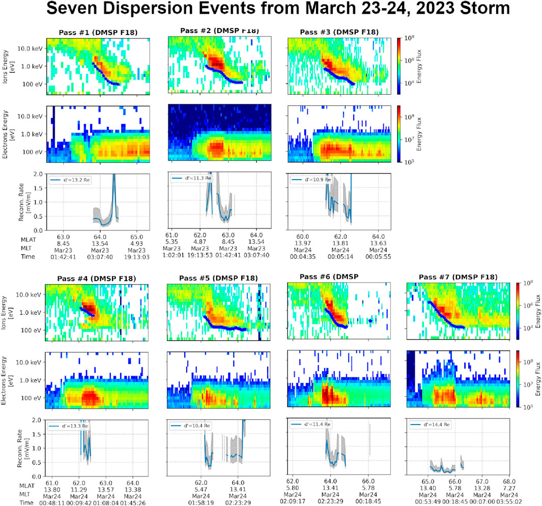
Figure 1. Consecutive ion-energy dispersion events made with DMSP F18 during the March 23–24, 2023 Geomagnetic Storm, with their calculated reconnection rates. Reconnection rates are zoomed to the range of values where they are most certain. Error bars are drawn to with the calculation repeated using $d{E}_{ic}/dt\to d{E}_{ic}/dt\pm 50\%$, capturing a single source of uncertainty in $d{E}_{ic}/dt$ (Lockwood and Smith, 1992).

The DMSP SSJ instrument is sensitive to particles in a small range for each channel. This is smaller than the spacing between energy channels, and no particle flux data is measured between these sensitive regions. This constrains the precision that the lower energy cutoff can reasonably measure. Quantifying this uncertainty and propagating through the Lockwood formula shall be considered in the Calculation Analysis section.

Because of the DMSP inclined orbits, most of their dayside time is spent in the northern hemisphere and most of the nightside time in the southern hemisphere (Oliveira and Zesta, 2024). Therefore, for this study, we are restricted to the northern cusp for our analysis of dayside precipitation.

To connect DMSP observations to the upstream solar wind, we use the OMNI dataset at a 1-min cadence (King and Papitashvili, 2020). OMNI is a calculated measurement of the interplanetary magnetic field (IMF), solar wind density, and pressure at Earth’s bow shock derived from L1 measurements of these variables. Specifically, OMNI propagates these measurements from the L1 point to Earth’s bow shock using simple ballistic physics to provide a convenient derived variable for magnetospheric data analysis. OMNI uses data from two spacecraft: the Advanced Composition Explorer (ACE) (Stone et al., 1998) and Wind (Ogilvie and Desch, 1997; Ogilvie et al., 1995).

3 Observations

In Figure 1, we present the ion and electron spectrograms from the DMSP SSJ instrument on F18 for seven consecutive passes of the northern cusp. Each panel is a consecutive pass spaced about 101 min apart, as defined by the orbital period. For each subsequent pass, dispersion is apparent in the ion spectrogram, and an electron burst coincides with the ion dispersion. The electrons are not expected to display dispersion on the same time scale as the ions (da Silva et al., 2022). We note that the peak flux (color bar color) in each dispersion structure is generally between $10^7$ and $10^{8}1/({\mathrm{c}\mathrm{m}}^2\ast \mathrm{s}\ast \mathrm{s}\mathrm{r})$, but varies by about an order of magnitude between passes, suggesting differences in the amount of momentum transferred to accelerated ions in the upstream injection process.

IMF and SYM-H values during each event can be found in Table 1. It is statistically unlikely that each of these passes was triggered by transient reconnection that, by chance, coincided with the satellite’s cusp traversal. The more likely scenario is that continuous reconnection occurred throughout this period, perhaps with modulations during unobserved times, with the satellite sampling an often present process. Continuous reconnection processes have been established through remote observation of the aurora (Frey et al., 2003) and analysis of cusp dispersion (Trattner et al., 2015). During this storm, we also observed dispersion events from DMSP F16 and F17, similar to those seen in F18. For additional context on the IMF and Dst index during this storm, see Supplementary Appendix Section 1.1, and for the ionospheric potential and open/closed boundaries, see Supplementary Appendix Section 1.2.

Table 1

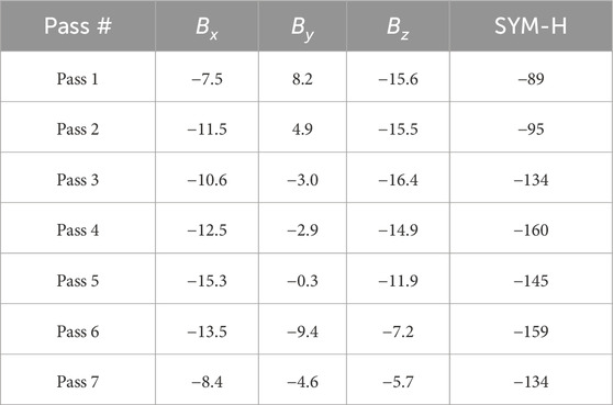
Table 1. OMNI IMF and SYM-H values during each event, in units of nT. IMF values are in GSM coordinates.

The spatial locations of the dispersion events are presented in a polar plot of the northern hemisphere in Figure 2. The precise magnetic local time (MLT) and magnetic latitude (MLAT) of the dispersion structures vary between passes as a function of the IMF (Petrinec et al., 2023) and solar wind dynamic pressure. The ion dispersion occurs in MLAT between $60°$ and $68°$, and MLT between 13.6 and 15.1. These locations are consistent with current knowledge of where the cusp may be placed. Detection locations from F16 and F17 are also shown in Figure 2 for comparison. It is expected that F16 and F17 detected fewer events than F18 because their orbits deviated further from noon MLT.

Figure 2

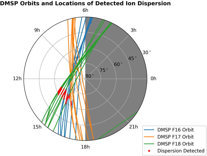
Figure 2. DMSP satellite (F16, F17, and F18) orbit tracks in magnetic coordinates during the event, with red highlights where dispersion events were detected. The cusp can be understood to be around the red detection region.

In the bottom panel of each dispersion event in Figure 1, a calculation of the reconnection rate is shown for multiple values of $d^{\prime }$. The variable $d^{\prime }$ is a free parameter of the calculation (to be explained later), representing the distance to the injection source virtually modified to account for parallel electric field acceleration. Because this is a free variable, we plot three curves for the range that may exist in practice ($10R_E$, $20R_E$, and $30R_E$). The calculated reconnection rates generally fall within the y-axis range, with some gaps. These gaps occur notably when the derivative of the blue curve in the top panel $(d{E}_{ic}/dt)$ equals zero, which causes the calculation to become numerically unstable due to a diminishing denominator. For this reason, we choose to exclude these points from the plots to avoid misinterpretation. The details of the calculation will be explained in the next section.

Error bars are drawn using the method from Lockwood and Smith (1992). This method, which addresses uncertainty in $d{E}_{ic}/dt$ only, is done by repeating the calculation with $d{E}_{ic}/dt$ replaced by versions with $\pm 50\%$ added. Due to the way $d{E}_{ic}/dt$ appears in the calculation, this results in larger error bars above the nominal value.

We observe from Figure 1 that the stable values are generally within 0.1–2 mV/m range. This range is commensurate values reported in previous work, such as Mozer and Retino (2007), where an average reconnection rate of 1.25 mV/m was calculated from eleven reconnection events using observations from the Magnetospheric Multiscale Mission (MMS) (Burch et al., 2016). It is also similar to (though slightly under) the estimated range of 3.2 $\pm$ 0.6 mV/m for the 11 July 2017 storm obtained using MMS observations in (Genestreti et al., 2018). The range of values within a panel can also, in a crude sense, be considered a scale of uncertainty associated with the calculation. Later, we will discuss how we trust the scale of the calculated values but not necessarily the fine variations within.

4 Calculation review

We will now discuss how the reconnection rate was calculated. The methodology for calculating the reconnection rate was first described in Lockwood and Smith (1992), and is reviewed here. The calculation inherently assumes that the dispersion is a temporal structure (Trattner et al., 2008), caused by the evolution of newly opened field lines.

For a parcel of ions arriving at the spacecraft, the time at which the parcel was injected onto the field line can be estimated as $\tau$ seconds ago, where $\tau$ is (Equation 1)

$\tau =d^{\prime }/\sqrt{2E_{ic}/m},(1)$

with $E_{ic}$ (ion cutoff energy) being the lower energy end of the parcel, $m$ being the mass of an ion, and $d^{\prime }$ being the virtual injection distance elongated for parallel acceleration. In this estimation, for the parcel of protons, $E_{ic}$ takes the role of $E_{\Vert }$.

Defining a coordinate system in the low altitude neighborhood of the spacecraft where $\widehat{x}$ is along the path of newly opened field lines and $\widehat{y}$ is perpendicular to it such that $\widehat{z}$ is facing away from Earth (see Lockwood and Smith (1992) Figure 1 for a diagram), we can estimate the traversal of the newly opened field line path by the satellite orbit with (Equation 2),

$dx/d{t}_s=V_s\mathrm{c}\mathrm{o}\mathrm{s}\left(\alpha \right),(2)$

where $t_s$ is the time in the satellite frame, $V_s$ is the speed of the satellite, and $\alpha$ is the angle between the spacecraft and $\widehat{x}$. At each instance, the injection occurred at $t_0=t_s-\tau$. The change in this with respect to $x$ is (Equation 3),

$d{t}_0/dx={\left(V_s\mathrm{c}\mathrm{o}\mathrm{s}\left(\alpha \right)\right)}^{-1}\left\{1+\left(d^{\prime }/2\right){\left(m/2\right)}^{1/2}{E}_{ic}^{-3/2}d{E}_{ic}/d{t}_s\right\}.(3)$

Using Faraday’s law, the rate at which flux is opened in an infinitesimal segment $dy$ is approximated by (Equation 4),

$B_{s}dxdy/d{t}_0=E_{y}dy=E_y^{\prime }d{y}^{\prime },(4)$

where $B_s$ is the magnetic field strength at the satellite, $E_y$ is the electric field at the satellite, $E_y^{\prime }$ is the reconnection rate, and $d^{\prime }$ is the length of the flux tube in the $y$ direction connecting to the current position of the satellite. The ratio $d{y}^{\prime }/dy$ relates the spatial width of the flux tube at the magnetopause to its smaller footprint at the satellite altitude. Pulling all these pieces together, the final equation for the reconnection rate is (Equation 5).

Magnetopause Reconnection Rate from Ion-Energy Dispersion Equation

$E_y^{\prime }=\left(\frac{d{y}^{\prime }}{dy}\right)\frac{B_s{V}_s\mathrm{c}\mathrm{o}\mathrm{s}\left(\alpha \right)}{1+\left(\frac{d^{\prime }}{2}\right)\sqrt{\frac{m}{2}}{E}_{ic}^{-3/2}\frac{d{E}_{ic}}{dt}}(5)$

5 Calculation analysis

The calculation outlined in Calculation Review requires estimating many variables to assemble a dayside reconnection model. While the variables like $V_s$ are easily obtainable, variables such as $d{y}^{\prime }/dy$, $\alpha$, $d^{\prime }$, and $E_{ic}$ are less straightforward. In this section, we summarize and discuss these variables and their related sources of uncertainty.

First, we address the FOV limitations of DMSP SSJ (5) before going forward. The FOV spans a $4°\times 90°$ fan and is not necessarily field aligned, which warrants consideration. Each instrument is mounted such that the $90°$ fan covers the ram direction to zenith and the $4°$ span is across the left-to-right side of the spacecraft. Based on the position and direction of the spacecraft throughout its orbit, this leads to non-sampling of pitch angle space when $\mathbf{B}$ is outside the $90°$ span and over-sampling when $\mathbf{B}$ is inside the $90°$ span.

The magnetometer data was compared with the instrument FOV for the two events for which magnetometer data. The pitch angle coverage was computed by calculating the angle between $\mathbf{B}$ and the vector pointing outward both ends of the fan (the ram direction and the zenith vector). The pitch angle coverage calculated this way was $101°$ to $162°$ for the first event and $122°$ to $143°$ for a second event, with variation in these values less than $2°$ within an event. We conclude that while this effect is important to understand, the implications are minor for the calculation presented here, because the under-sampling is consistent during an event and overall does not change the structure of the $E_{ic}$ curve used to deduce the reconnection rate.

The ion energy cutoff $E_{ic}$ is a significant source of uncertainty with DMSP. Lockwood and Smith (1992) recommends using the energy that produces 10% of the peak flux in the energy spectra, though in practice, this is complicated to apply. In Figure 3, we display a sample set of energy spectra from a dispersed ion population. We have drawn a horizontal dashed line at the level of 10% of the peak flux. In several of these time steps, we point out that calculating the cutoff energy this way is difficult due to issues like out of population low energy counts, non-unimodal distributions, or the fact that finding that energy would require extrapolation. We tested alternative thresholds (5% and 15%) and found that they yielded comparable results, though values under 5% are more susceptible to out of population low energy counts.

Figure 3

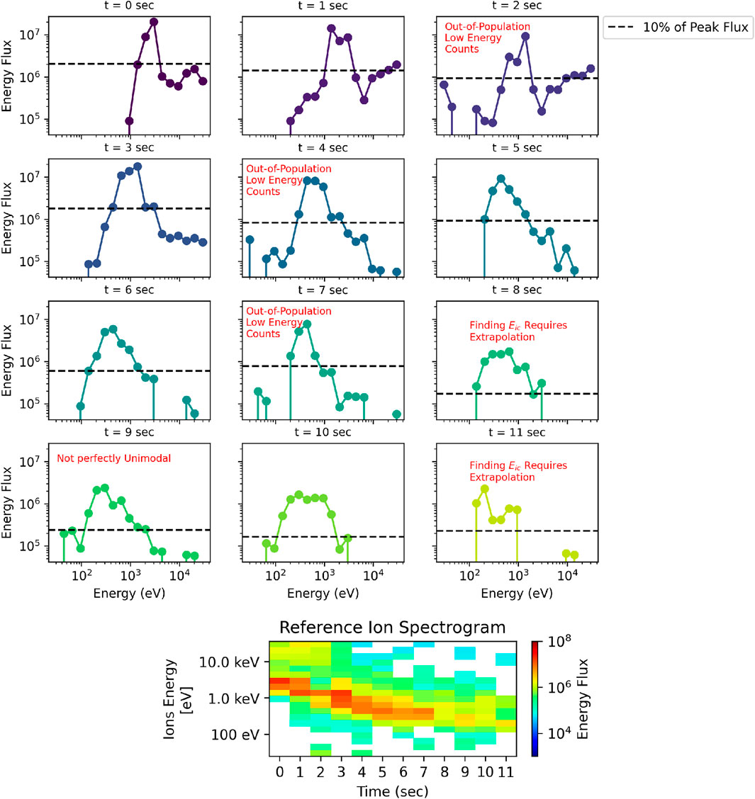
Figure 3. Illustration of a major source of uncertainty in calculating the reconnection rate with DMSP, which is picking the $E_{ic}$ value (ion cutoff energy).

We note that other work on the cusp has calculated the ion energy cutoff by fitting a Gaussian distribution to the distribution function $f(v_{\Vert })$ where $v_{\Vert }$ is the parallel velocity and $f$ is the distribution function. The approach then takes $1/e$ times the gaussian’s peak energy as the cut-off (Trattner et al., 2005a). However, this method is unavailable when using DMSP due to the lack of 3D distribution functions. In Figure 1, we smoothed the $E_{ic}(t)$ time series using a moving average window of five total points to minimize the effects of noise, as previously done in da Silva et al. (2022).

Regarding the width scaling between ends of flux tube $(d{y}^{\prime }/dy)$, Lockwood and Smith (1992) recommends taking nominal values of upstream and downstream the magnetic field strength and comparing the areas required to conserve magnetic flux. That is, setting ${\mathrm{\Phi }}_{mp}={\mathrm{\Phi }}_s$ where ${\mathrm{\Phi }}_{mp}$ and ${\mathrm{\Phi }}_s$ are the magnetic fluxes through the magnetopause and satellite altitude cross-sections of the flux tube, respectively. In this formulation, the width scaling is (Equation 6):

$\frac{d{y}^{\prime }}{dy}\approx \sqrt{\frac{B_s}{B_{mp}}},(6)$

where $B_{mp}$ is the nominal magnetic field strength at the magnetopause, and $B_s$ is the nominal (or measured) magnetic field strength at the satellite altitude. The upstream magnetopause magnetic field strength is difficult to obtain without a conjunction, so a back-of-the-envelope values of 50 nT for the satellite and 50,000 nT for the magnetopause are suggested. This produces a value of $\approx 31.6$. However, for the three events in Figure 1 for which magnetometer was available, the range of $B_s$ at the satellite was between 30,000 and 42,000 nT. In the absence of magnetometer data, it is recommended to obtain $B_s$ from the dipole equation (Equation 7)

$B_s=B_0{\left(\frac{R_E}{R_E+h}\right)}^3\sqrt{1+3{\mathrm{c}\mathrm{o}\mathrm{s}}^2\left(\theta \right)},(7)$

where $B_0$ is the mean value of the magnetic field at the magnetic equator (around 31,000 nT), $R_E$ is the radius of the Earth, $h$ is the spacecraft altitude (around 840 km), and $\theta$ is the magnetic colatitude measured from the north magnetic pole.

The distance between the injection source with parallel acceleration $d^{\prime }$ is primarily affected by varying levels of dayside compression from the solar wind dynamic pressure and the intensity of the parallel electric field $E_{\Vert }$ across the transit path. Previous work has suggested that large-scale parallel electric fields may occur throughout the dayside during magnetic reconnection (Egedal et al., 2012), emphasizing the need to adjust $d\to d^{\prime }$ for $E_{\Vert }$. This variable is expected to vary between $10R_E$ and $30R_E$ (Lockwood and Smith, 1992)., depending on factors like solar wind dynamic pressure and the corresponding compression of the dayside magnetosphere.

The angle between the spacecraft and the direction at which new field lines are opened is denoted by $\alpha$. For purely southward reconnection with an x-line across the magnetic equator, $\alpha$ is the angle between the spacecraft velocity and the closest line of latitude. However, this is rarely the case and inappropriate for reconnection scenarios involving off-equator x-lines, such as when a substantial $B_y$ component is present. The determination of $\alpha$ in the general case can be performed with the aid of modeling.

Such modeling includes the determination of the x-line location, such as through an analysis of the magnetic shear between the magnetosheath and the magnetosphere. A magnetic shear analysis for our events is presented in Figure 4. In this plot, the well-established Maximum Magnetic Shear model (Trattner et al., 2017). Figure 4 plots the magnetic shear across the magnetopause in the colored background, and plots the x-line as a gray line. In this model, the magnetosheath magnetic field is calculated using an analytic model based on upstream measurements made by Wind Kobel and Flückiger (1994), the magnetospheric magnetic field is estimated with the semi-empirical Tsyganenko 1995 model often abbreviated as T96 (Tsyganenko, 1995), and the magnetic shear is the angle between the two.

Figure 4

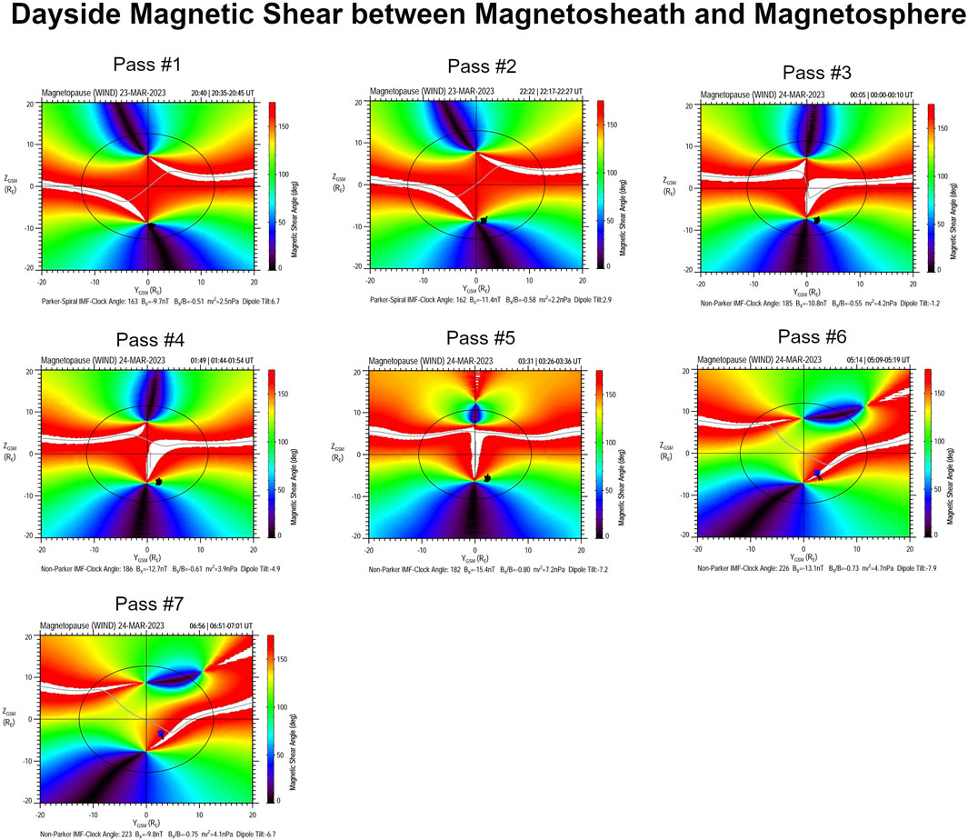
Figure 4. Magnetic Shear between the magnetosheath and magnetospheric magnetic field as calculated using the Maximum Magnetic Shear Model (Trattner et al., 2017). The passes identified in the title of each panel correspond to those labeled in Figure 1.

Each panel is calculated using the closest available output to the corresponding pass. Specifically, we refer to cases represented in passes #6 and#7, where the location of the x-line suggests strong longitudinal field line convection. In these cases, in the absence of ion drift and magnetometer data, considering $\alpha$ as a higher angle such as $45°$ or $60°$ is more accurate than the default $0°$. Later, we will show that $\alpha$ obtained using $\mathbf{E}=-\mathbf{v}\times \mathbf{B}$ and the spacecraft velocity vector agrees with this statement for pass #7 (no magnetometer is available to test pass #6).

To study the effect of $\alpha$ further, we varied $\alpha$ between 0 and 75$°$ in increments of 15$°$ and recalculated the reconnection rate using a nominal $d^{\prime }=20R_E$. At $\alpha =90°$, the calculation fails since no time-dependent dispersion is observed, making Equation 5 zero. The result of this exercise can be seen in Figure 5. We observe that underestimating $\alpha$ leads to over-estimating the reconnection rate, with the maximum relative difference between 75$°$ and 0$°$ being a factor of 3.86 and the maximum absolute difference being 0.91 mV/m.

Figure 5

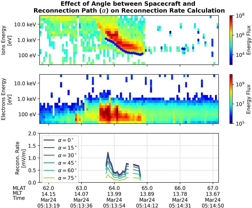
Figure 5. Illustration of the effects of varying $\alpha$, the angle between the spacecraft and the direction of newly opened field lines, on the reconnection rate calculation. This variable cannot be measured directly by DMSP, and for the purposes of using DMSP it is a free variable in the calculation.

We also note that in Figure 1, the values of $d^{\prime }$ used were obtained using field line traces in a magnetic field model produced through a MAGE (v0.75) simulation. The traces aimed to find the distance between the satellite and the three dimensional x-line, as dictated by the Maximum Magnetic Shear model. Values of $d^{\prime }$ found this way ranged between $10.4R_E$ and $14.4R_E$ for this storm. Specifically, a field line was first traced starting through the satellite location. When this field line did not intersect the x-line, the starting position was moved outward to find the closest field line that did. The final distance was then taken as the closest point on that field line between the satellite location and the x-line.

As a point of discussion, we note that the calculation is intrinsically temporally limited overall. A 100 eV field-aligned proton takes 11.5 min to travel 15 $R_E$, while a 10 keV proton takes 1.2 min. To this effect, extracting a single value for the reconnection rate from ion-energy dispersion condenses a process on the time scale of 10 min into each timestep of the reconnection rate time series in Figure 1.

6 Comparison to $\mathbf{v}\times \mathbf{B}$ baseline

In this section, we sanity-check the calculation results from the previous sections using an alternate method. The comparison made in this section will justify the order of magnitude. Still, because of the comparison methodology’s limitations, it cannot justify any more minor time-scale features in the reconnection rate curve.

The method we compare as a baseline utilizes DMSP’s SSM magnetometer and the SSIES IDM ion drift measurements. Using the Ohm’s law approximation, we calculate $|\mathbf{E}|$ at the satellite location using the approximation that $\mathbf{E}\approx -\mathbf{v}\times \mathbf{B}$. Then, following a similar methodology to the Lockwood formulation, we apply the flux tube width scaling factor $d{y}^{\prime }/dy$ to obtain the magnetopause reconnection rate from the ionospheric electric field. The final formula is (Equation 8).

Magnetopause Reconnection Rate from $\mathbf{v}\times \mathbf{B}$ Baseline Equation

$E_y^{\prime }\approx \left(\frac{d{y}^{\prime }}{dy}\right)|\mathbf{v}\times \mathbf{B}|(8)$

where $d{y}^{\prime }/dy$ is identical to that used in the Lockwood formulation, $\mathbf{v}$ is the ion drift measurement, $\mathbf{B}$ is the magnetometer measurement, and $E_y^{\prime }$ is the magnetopause reconnection rate.

In Figure 6, we compare the reconnection rate from the Lockwood method with that of the baseline for passes #2 and #7. In both cases, the reconnection rate curves produced by the $\mathbf{v}\times \mathbf{B}$ method and the Lockwood method agree on order of magnitude, although fine structure is not shared. From this comparison, we conclude that the calculated reconnection rate using the Lockwood method is the correct order of magnitude, up to and excluding the $d{y}^{\prime }/dy$ flux tube width scaling term.

Figure 6

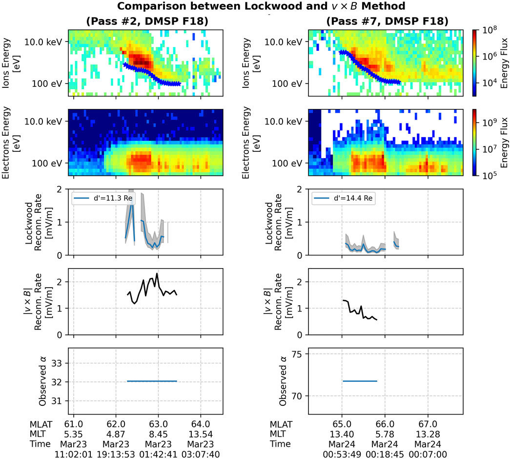
Figure 6. Comparison between the Lockwood Method and the $\mathbf{v}\times \mathbf{B}$ method. While the reconnection rate curves produced by the $\mathbf{v}\times \mathbf{B}$ method show some differences in structure with the curved produced by the Lockwood method, they is the same order of magnitude. The reconnection rate from the Lockwood method computed here uses the observed $\alpha$.

We also present the observed $\alpha$, calculated as the angle between the previously defined $x$ axis and the spacecraft trajectory.

The DMSP SSM and SSIES instruments use a coordinate system where $+x^{\prime }$ is in the vertical direction, $+y^{\prime }$ is in the direction of the spacecraft velocity, and $+z^{\prime }$ completes the right-handed system (pointing to the right side of the spacecraft). We compute $\alpha$ as the remainder between a right angle and the angle between $\mathbf{E}$ and the satellite velocity both projected onto the $y^{\prime }-z^{\prime }$ plane (Equation 9),

$\alpha \approx 90°-{\mathrm{c}\mathrm{o}\mathrm{s}}^{-1}\left(\frac{E_{y^{\prime }}}{\sqrt{E_{y^{\prime }}^2+E_{z^{\prime }}^2}}\right).(9)$

For reference, if $\mathbf{E}$ and the satellite velocity are perpendicular in the $y^{\prime }-z^{\prime }$ plane, then $\alpha =0°$. We compute $\alpha$ this way for passes with available magnetometer data, #2 and #7. In Figure 1, we use a value of $\alpha =0°$ for the others where no magnetometer data is available. The curve in Figure 6 uses these $\alpha$’s to calculate the reconnection rate. The average $\alpha$ value computed this way is $32.0°$ for pass #2 and $71.7°$ degrees for pass #7. This agrees with our previous statement that based on the magnetic shear plot in Figure 4 for pass #7, $\alpha$ should be higher the other passes.

7 Conclusion

In this work, we applied the Lockwood and Smith (1992) method to calculate the dayside reconnection rate using dispersion ion-energy cusp signatures observed by the DMSP satellites. By analyzing dispersion present in seven consecutive passes during a time of continuous southward IMF reconnection in the March 23–24, 2024, geomagnetic storm, we demonstrated the feasibility of applying DMSP SSJ data to study storm-time reconnection rates and found a largely consistent reconnection rate during the main phase of the March 23–24, 2024 geomagnetic storm.

We note that a limitation of using DMSP for the calculation described here revolves around the space-time ambiguity. The Lockwood method assumes a temporal structure causes the dispersion, but it is impossible to distinguish between temporal and spatial structures with DMSP. This work is presented in the hope that results from improved instrumentation on the TRACERS mission and ground radar will provide enhanced understanding on the role and rate of temporal versus cusp structures. For instance, information such as how rare/common one is compared to the other would change the landscape of applying the methodology. If it is concluded that temporal structures appear in orbit at a rate significantly more frequently than spatial structures, then for certain space weather applications the benefits of applying the methodology may outweigh the cost of accepting some misapplications.

In future work, this methodology could be extended to other spacecraft or combined with ground-based radar. Ground-based radars, such as the Super Dual Auroral Radar Network (SuperDARN) (Greenwald et al., 1995; Chisham et al., 2007), have previously been used to measure the ionospheric electric field and calculate the dayside reconnection voltage (de La Beaujardiere et al., 1991; Hubert et al., 2006). Other spacecraft in higher orbits, such as Cluster, also traverse the high altitude cusp (beyond 2 $R_E$) and observe ion-energy dispersion. The main advantage of Cluster compared to DMSP is that of superior instrumentation, including the ability to provide 3-D velocity distribution functions; the downside is the longer orbital period, which limits the number of cusp traversals during a geomagnetic storm.

Our results indicate the calculated reconnection rates with DMSP during this storm were generally between 0.1 and 2 mV/m, when very uncertain (usually higher) values are excluded. This range of values is similar to previous estimations of the reconnection rates during geomagnetic storms obtained using in-situ MMS observations (Mozer and Retino, 2007; Genestreti et al., 2018). In this manuscript, we extended the previous discussion in the literature on uncertainty sources for the Lockwood method, such as the determination of the ion cutoff energy $(E_{ic})$, the angle between the reconnection path and the spacecraft trajectory $(\alpha )$, and the virtual distance to the injection site $(d^{\prime })$. Despite these sources of uncertainty, our comparison to a method that produces a first-order estimate of the reconnection rate using $|\mathbf{E}|=|\mathbf{v}\times \mathbf{B}|$ to approximate the local electric field confirmed that our results are on the correct order of magnitude, up to the $d{y}^{\prime }/dy$ flux tube width scaling term required for both calculations.

This work highlights the potential for long-term statistical studies of the reconnection using the extensive multi-decade DMSP dataset, should we come to a point where the assumption of temporal structure can be justified on a case to case basis. Future instrumentation, such as that which will fly with the TRACERS mission, will provide an opportunity to further test the Lockwood method. An avenue for future work during the TRACERS era is the study of other storms with more pronounced changes in the reconnection rate during the main phase.

Data availability statement

The original contributions presented in the study in the form of code and associated data are publicly available. They can be found on Zenodo at https://doi.org/10.5281/zenodo.15660989

Author contributions

DS: Software, Conceptualization, Methodology, Formal Analysis, Writing – original draft, Writing – review and editing, Investigation. LC: Methodology, Conceptualization, Writing – review and editing, Writing – original draft. SF: Writing – review and editing, Methodology. KT: Methodology, Writing – review and editing. BB: Methodology, Writing – review and editing. ID: Writing – review and editing, Methodology. NB: Methodology, Data curation, Writing – review and editing. JD: Writing – review and editing.

Funding

The author(s) declare that financial support was received for the research and/or publication of this article. This work was supported by NASA.

Conflict of interest

The authors declare that the research was conducted in the absence of any commercial or financial relationships that could be construed as a potential conflict of interest.

The author(s) declared that they were an editorial board member of Frontiers, at the time of submission. This had no impact on the peer review process and the final decision.

Generative AI statement

The author(s) declare that no Generative AI was used in the creation of this manuscript.

Publisher’s note

All claims expressed in this article are solely those of the authors and do not necessarily represent those of their affiliated organizations, or those of the publisher, the editors and the reviewers. Any product that may be evaluated in this article, or claim that may be made by its manufacturer, is not guaranteed or endorsed by the publisher.

Supplementary material

The Supplementary Material for this article can be foundonline at: https://www.frontiersin.org/articles/10.3389/fspas.2025.1607611/full#supplementary-material

References

Alken, P., Maus, S., Lühr, H., Redmon, R., Rich, F., Bowman, B., et al. (2014). Geomagnetic main field modeling with DMSP. J. Geophys. Res. Space Phys. 119, 4010–4025. doi:10.1002/2013ja019754

CrossRef Full Text | Google Scholar

Balogh, A., Dunlop, M., Cowley, S., Southwood, D., Thomlinson, J., Glassmeier, K., et al. (1997). The Cluster magnetic field investigation. Space Sci. Rev. 79, 65–91. doi:10.1007/978-94-011-5666-0_3

CrossRef Full Text | Google Scholar

Basinska, E. M., Burke, W. J., Maynard, N. C., Hughes, W., Winningham, J., and Hanson, W. (1992). Small-scale electrodynamics of the cusp with northward interplanetary magnetic field. J. Geophys. Res. Space Phys. 97, 6369–6379. doi:10.1029/91ja03023

CrossRef Full Text | Google Scholar

Burch, J., Moore, T., Torbert, R., and Giles, B.-h. (2016). Magnetospheric multiscale overview and science objectives. Space Sci. Rev. 199, 5–21. doi:10.1007/s11214-015-0164-9

CrossRef Full Text | Google Scholar

Chisham, G., Lester, M., Milan, S., Freeman, M., Bristow, W., Grocott, A., et al. (2007). A decade of the super dual auroral radar network (superdarn): scientific achievements, new techniques and future directions. Surv. Geophys. 28, 33–109. doi:10.1007/s10712-007-9017-8

CrossRef Full Text | Google Scholar

Connor, H., Raeder, J., Sibeck, D., and Trattner, K. (2015). Relation between cusp ion structures and dayside reconnection for four IMF clock angles: OpenGGCM-LTPT results. J. Geophys. Res. Space Phys. 120, 4890–4906. doi:10.1002/2015ja021156

CrossRef Full Text | Google Scholar

Connor, H., Raeder, J., and Trattner, K. (2012). Dynamic modeling of cusp ion structures. J. Geophys. Res. Space Phys. 117. doi:10.1029/2011ja017203

CrossRef Full Text | Google Scholar

da Silva, D., Chen, L., Fuselier, S., Petrinec, S., Trattner, K., Cucho-Padin, G., et al. (2024). Statistical analysis of overlapping double ion energy dispersion events in the northern cusp. Front. Astronomy Space Sci. 10, 1228475. doi:10.3389/fspas.2023.1228475

CrossRef Full Text | Google Scholar

da Silva, D., Chen, L., Fuselier, S., Wang, S., Elkington, S., Dorelli, J., et al. (2022). Automatic identification and new observations of ion energy dispersion events in the cusp ionosphere. J. Geophys. Res. Space Phys. 127, e2021JA029637. doi:10.1029/2021ja029637

CrossRef Full Text | Google Scholar

King, J. H., and Papitashvili, N. E. (2020). Omni 1-min data set. doi:10.48322/45BB-8792

CrossRef Full Text | Google Scholar

de La Beaujardiere, O., Lyons, L., and Friis-Christensen, E. (1991). Sondrestrom radar measurements of the reconnection electric field. J. Geophys. Res. Space Phys. 96, 13907–13912. doi:10.1029/91ja01174

CrossRef Full Text | Google Scholar

Egedal, J., Daughton, W., and Le, A. (2012). Large-scale electron acceleration by parallel electric fields during magnetic reconnection. Nat. Phys. 8, 321–324. doi:10.1038/nphys2249

CrossRef Full Text | Google Scholar

Frey, H., Phan, T., Fuselier, S., and Mende, S. (2003). Continuous magnetic reconnection at Earth’s magnetopause. Nature 426, 533–537. doi:10.1038/nature02084

PubMed Abstract | CrossRef Full Text | Google Scholar

Fuselier, S., Klumpar, D., and Shelley, E. (1991). Ion reflection and transmission during reconnection at the Earth’s subsolar magnetopause. Geophys. Res. Lett. 18, 139–142. doi:10.1029/90gl02676

CrossRef Full Text | Google Scholar

Fuselier, S., Petrinec, S., and Trattner, K. (2000). Stability of the high-latitude reconnection site for steady northward IMF. Geophys. Res. Lett. 27, 473–476. doi:10.1029/1999gl003706

CrossRef Full Text | Google Scholar

Genestreti, K. J., Nakamura, T., Nakamura, R., Denton, R. E., Torbert, R. B., Burch, J. L., et al. (2018). How accurately can we measure the reconnection rate em for the mms diffusion region event of 11 july 2017? J. Geophys. Res. Space Phys. 123, 9130–9149. doi:10.1029/2018ja025711

PubMed Abstract | CrossRef Full Text | Google Scholar

Greenwald, R., Baker, K., Dudeney, J., Pinnock, M., Jones, T., Thomas, E., et al. (1995). Darn/superdarn: a global view of the dynamics of high-latitude convection. Space Sci. Rev. 71, 761–796. doi:10.1007/bf00751350

CrossRef Full Text | Google Scholar

Hubert, B., Milan, S., Grocott, A., Blockx, C., Cowley, S., and Gérard, J.-C. (2006). Dayside and nightside reconnection rates inferred from image fuv and super dual auroral radar network data. J. Geophys. Res. Space Phys. 111. doi:10.1029/2005ja011140

CrossRef Full Text | Google Scholar

Kihn, E., Redmon, R., Ridley, A., and Hairston, M. (2006). A statistical comparison of the AMIE derived and DMSP-SSIES observed high-latitude ionospheric electric field. J. Geophys. Res. Space Phys. 111. doi:10.1029/2005ja011310

CrossRef Full Text | Google Scholar

Kletzing, C. (2019). The Tandem reconnection and cusp electrodynamics reconnaissance satellites (TRACERS) mission. AGU Fall Meet. Abstr. 2019, A41U–2687.

Google Scholar

Kobel, E., and Flückiger, E. (1994). A model of the steady state magnetic field in the magnetosheath. J. Geophys. Res. Space Phys. 99, 23617–23622. doi:10.1029/94ja01778

CrossRef Full Text | Google Scholar

Lockwood, M., and Smith, M. (1992). The variation of reconnection rate at the dayside magnetopause and cusp ion precipitation. J. Geophys. Res. Space Phys. 97, 14841–14847. doi:10.1029/92ja01261

CrossRef Full Text | Google Scholar

Lockwood, M., and Smith, M. F. (1989). Low-altitude signatures of the cusp and flux transfer events. Geophys. Res. Lett. 16, 879–882. doi:10.1029/gl016i008p00879

CrossRef Full Text | Google Scholar

Mozer, F., and Retino, A. (2007). Quantitative estimates of magnetic field reconnection properties from electric and magnetic field measurements. J. Geophys. Res. Space Phys. 112. doi:10.1029/2007ja012406

CrossRef Full Text | Google Scholar

Ogilvie, K., Chornay, D., Fritzenreiter, R., Hunsaker, F., Keller, J., Lobell, J., et al. (1995). SWE, a comprehensive plasma instrument for the Wind spacecraft. Space Sci. Rev. 71, 55–77. doi:10.1007/bf00751326

CrossRef Full Text | Google Scholar

Ogilvie, K., and Desch, M. (1997). The wind spacecraft and its early scientific results. Adv. Space Res. 20, 559–568. doi:10.1016/s0273-1177(97)00439-0

CrossRef Full Text | Google Scholar

Oliveira, D. M., and Zesta, E. (2024). Inter-hemispheric energy input into the ionosphere-thermosphere system during magnetic storms: what we can and cannot learn from DMSP observations. J. Geophys. Res. Space Phys. 129, e2024JA032486. doi:10.1029/2024ja032486

CrossRef Full Text | Google Scholar

Petrinec, S., Kletzing, C., Bounds, S., Fuselier, S., Trattner, K., and Sawyer, R. (2023). TRICE-2 rocket observations in the low-altitude cusp: boundaries and comparisons with models. J. Geophys. Res. Space Phys. 128, e2022JA030952. doi:10.1029/2022ja030952

CrossRef Full Text | Google Scholar

Redmon, R. J., Denig, W. F., Kilcommons, L. M., and Knipp, D. J. (2017). New DMSP database of precipitating auroral electrons and ions. J. Geophys. Res. Space Phys. 122, 9056–9067. doi:10.1002/2016ja023339

PubMed Abstract | CrossRef Full Text | Google Scholar

Stone, E. C., Frandsen, A., Mewaldt, R., Christian, E., Margolies, D., Ormes, J., et al. (1998). The advanced composition explorer. Space Sci. Rev. 86, 1–22. doi:10.1007/978-94-011-4762-0_1

CrossRef Full Text | Google Scholar

Torbert, R., Russell, C., Magnes, W., Ergun, R., Lindqvist, P.-A., LeContel, O., et al. (2016). The FIELDS instrument suite on MMS: scientific objectives, measurements, and data products. Space Sci. Rev. 199, 105–135. doi:10.1007/978-94-024-0861-4_5

CrossRef Full Text | Google Scholar

Trattner, K., Burch, J., Ergun, R., Eriksson, S., Fuselier, S., Giles, B., et al. (2017). The MMS dayside magnetic reconnection locations during phase 1 and their relation to the predictions of the maximum magnetic shear model. J. Geophys. Res. Space Phys. 122, 11–991. doi:10.1002/2017ja024488

CrossRef Full Text | Google Scholar

Trattner, K., Fuselier, S., Peterson, W., Boehm, M., Klumpar, D., Carlson, C., et al. (2002). Temporal versus spatial interpretation of cusp ion structures observed by two spacecraft. J. Geophys. Res. Space Phys. 107, SMP–9. doi:10.1029/2001ja000181

CrossRef Full Text | Google Scholar

Trattner, K., Fuselier, S., Peterson, W., Sauvaud, J.-A., Stenuit, H., Dubouloz, N., et al. (1999). On spatial and temporal structures in the cusp. J. Geophys. Res. Space Phys. 104, 28411–28421. doi:10.1029/1999ja900419

CrossRef Full Text | Google Scholar

Trattner, K., Fuselier, S., Petrinec, S., Yeoman, T., Mouikis, C., Kucharek, H., et al. (2005a). Reconnection sites of spatial cusp structures. J. Geophys. Res. Space Phys. 110. doi:10.1029/2004ja010722

CrossRef Full Text | Google Scholar

Trattner, K., Fuselier, S., Petrinec, S., Yeoman, T. K., Escoubet, C., and Reme, H. (2008). The reconnection site of temporal cusp structures. J. Geophys. Res. Space Phys. 113. doi:10.1029/2007ja012776

CrossRef Full Text | Google Scholar

Trattner, K., Fuselier, S., Yeoman, T., Carlson, C., Peterson, W., Korth, A., et al. (2005b). Spatial and temporal cusp structures observed by multiple spacecraft and ground based observations. Surv. Geophys. 26, 281–305. doi:10.1007/1-4020-3605-1_12

CrossRef Full Text | Google Scholar

Trattner, K., Onsager, T., Petrinec, S., and Fuselier, S. (2015). Distinguishing between pulsed and continuous reconnection at the dayside magnetopause. J. Geophys. Res. Space Phys. 120, 1684–1696. doi:10.1002/2014ja020713

PubMed Abstract | CrossRef Full Text | Google Scholar

Tsyganenko, N. A. (1995). Modeling the earth’s magnetospheric magnetic field confined within a realistic magnetopause. J. Geophys. Res. Space Phys. 100, 5599–5612. doi:10.1029/94ja03193

CrossRef Full Text | Google Scholar