Optimizing Dryland Crop Management to Regional Climate. Part II: U.S. Southern High Plains Grain Sorghum Production

Introduction

Over the U.S. Southern High Plains (SHP) sorghum [Sorghum bicolor (L.) Moensch] plays an important part in un-irrigated “dryland” agricultural production. During 2016–2018 Texas was the second-ranked U.S. state behind Kansas in planted sorghum acres [NASS (U. S. Department of Agriculture National Agricultural Statistics Service), 2019], with a major production area located in the Texas Panhandle-SHP region. Sorghum's heat and drought tolerance make it well-suited to the area's semi-arid summer growing conditions, and its genetic diversity makes the crop potentially useful as forage, a gluten-free grain source, and in biofuel production (Dahlberg et al., 2011). Over the broader southern Ogallala aquifer region it is a major feed grain and silage source to the area's confined livestock operations (Amosson et al., 2014). Although cotton is currently the main SHP summer crop, sorghum is the leading alternative for producers in years when dryland cotton fails due to dry conditions, heat stress, or hail damage. With the ongoing depletion of the Ogallala aquifer (Sophocleous, 2010; Haacker et al., 2016; McGuire, 2017) the region's agricultural economy may be increasingly dependent on un-irrigated production in the future. As a result, there is need to explore and define best dryland management practices for both crops in the region's growing environment.

However, natural variation in summer rainfall makes it hard to identify best management options for SHP dryland crops. In semi-arid regions un-irrigated yields are largely determined by the amount and timing of rainfall, which can vary considerably and unpredictably from year to year. This uncertainty in rainfall leads to uncertainty in both yields and profits. Although seasonal precipitation forecasts might allow producers to pro-actively manage planting by providing advance notice of a wet or dry growing season, over the central U.S. the prospects for predicting summer rainfall are limited (Livezey and Timofeyeva, 2008; Peng et al., 2012). Given the inability to predict seasonal rainfall, an alternative is to “manage to climatology,” i.e., identify and adopt crop-specific management practices that are optimal to a growing region's current climate conditions. Because rainfall is the leading driver of variability in dryland yields and profits, identifying climate-optimal practices and estimating the associated production risk requires an extensive sampling of growing season rainfall outcomes, and a way of translating those outcomes into crop yields. One way to make this connection is multiple-year field experiments at multiple sites, which might sample a wide range of seasonal rainfall variability and produce a corresponding range of yields. But the resources required by such field experiments would be considerable, particularly when repeated over a range of management options. Another option is to use crop models to simulate production over a representative range of current dryland growing conditions.

In a preceding companion paper (Mauget et al., 2019; hereafter M19) a modeling-based method was demonstrated that identified climate-optimal practices in SHP dryland cotton production. Here, this approach is applied to dryland sorghum production. In this scheme a crop model is used to translate large samples of growing season weather outcomes into dense distributions of simulated yield outcomes. As the weather data inputs to the CERES-Sorghum model used here are limited here to records during 2005–2016, that data, and the resulting modeled grain yield distributions, are considered representative of current SHP summer climate. Optimal management practices for current climate are sought by repeating simulations over a range of management options to identify those that maximize median yield. The densely-sampled yield distributions can be used to estimate the probability of dryland yield outcomes under current conditions. Given assumed commodity prices and production costs, they also might be used to estimate the probability of profit outcomes. The key component in this process that makes the estimation of current production risk possible is the use of 11 years of weather data inputs from 21 West Texas Mesonet (WTM) weather stations (Schroeder et al., 2005). This broad sampling of seasonal rainfall outcomes generates 231 yields for each management option, which in turn estimate the climate-driven variation in current SHP dryland sorghum production. In addition to allowing for estimates of dryland production risk at high resolution, this process can also generate similarly resolved yield effect (Δ_Y) distributions resulting from the choice of one management option over another.

Previous sorghum simulations (Chapman et al., 2000; Hammer, 2006; Hammer et al., 2014) have explored how genetics and management might be optimized to different Australian production environments. The modeling approach followed here is generally similar to that found in Hammer et al. (2014), hereafter, H14, but differs in some respects. Whereas, H14 modeled yields from 405 possible genetic variations over 5 environment types, the focus here is on one medium maturity cultivar grown in the SHP environment. However, both here and in H14 more than 100 station-years of weather data were used to generate yield ensembles to estimate yield risk for a range of management options. In addition, the emphasis in H14 and the current study is on simulating yield effects due to rainfall variation, which is the main production-limiting factor in both Australian and SHP dryland sorghum production.

The following Materials and Methods section describes the CERES-Sorghum model, its calibration based on SHP field studies, and the model's weather data inputs and initial conditions. That section concludes by outlining the simulation's experimental design, and compares CERES-Sorghum yield statistics vs. recent regional production statistics. The Results section presents the simulated grain yield distributions of 32 sorghum management options and describes management-related yield effects. The Summary and Discussion section summarizes and discusses results, outlines recommendations for SHP dryland sorghum management, and previews related future research.

Materials and Methods

The CERES-Sorghum Model

CERES-Sorghum (Alagarswamy and Ritchie, 1991; White et al., 2015) is the sorghum growth module of the Decision Support System for Agrotechnology Transfer cropping system model (DSSAT-CSM) (Jones et al., 2003; Hoogenboom et al., 2017). As described in greater detail in Jones et al. (2003), the DSSAT-CSM is an integrated collection of software components that includes a main program, management module, soil module, weather module, and a soil-plant-atmosphere module. The model simulates plant growth processes at daily time steps and requires daily weather inputs. In the version used here (4.6.1.0) crop-specific growth modules simulate the development of 45 individual crops. Each crop growth module requires environmental data, genetic and ecotype parameters, and crop management parameters as inputs. A more complete description of the CERES-Sorghum growth module, and its ability to reproduce sorghum phenology, yield variation, and management effects found in field studies can be found in White et al. (2015).

Model Calibration

The CERES-Sorghum growth parameters used here were estimated by Kothari et al. (2019) based on field trials conducted at Texas A&M University's AgriLife Research Center at Halfway, TX. The Halfway sorghum trials were carried out during 2007, 2010, 2012, and 2013 under low, base, and high irrigation rates (Bordovsky et al., 2013). The trials's medium-maturity grain cultivars varied during those years, with the DeKalb variety DKS 44-20 planted in 2010 and 2012, DKS 37-07 in 2007, and DKS 49-45 in 2013. The medium-maturity cultivar and ecotype parameters used here for CERES-Sorghum were calculated based on a step-wise procedure that adjusted parameters to reproduce yields and the timing of growth stages in the high irrigation trials. Model validation was carried out by testing CERES-Sorghum's ability to reproduce yields in the low- and base-irrigated trials using those parameters (Kothari et al., 2019). The comparison of simulated and observed yields from the validation trials resulted in an r² of 0.86 and an index of agreement (d) of 0.96.

Weather Data Inputs and Simulation Initial Conditions

To allow for the comparison of dryland cotton and sorghum profit and risk outcomes in subsequent work, the CERES-Sorghum simulations for each station-year were driven using the same WTM weather data used to generate the M19 dryland cotton simulations. As described in M19, the daily weather inputs from each of Figure 1's 21 weather stations were derived by averaging or summing sub-daily WTM data into daily values, or defining daily maximum and minimum temperatures based on the WTM's reported 5 min temperature records. The resulting daily weather inputs include minimum and maximum temperature at 2.0 m, average dew point temperature, total precipitation, total solar radiation, and 2.0 m daily wind run. The archived 5 min WTM data records were subjected to the quality control (QC) procedures described in Schroeder et al. (2005), while the daily values calculated here were subjected to additional QC tests described by Mauget et al. (2017).

FIGURE 1

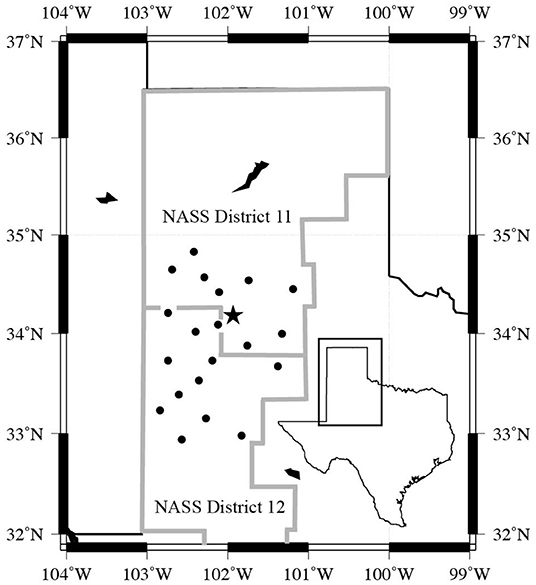
Figure 1. Locations of the 21 mesonet weather stations used to provide weather input data for the CERES-Sorghum model during 2005–2016. Star marks the location of the Texas A&M AgriLife Research Center at Halfway, Texas.

The dryland sorghum crop simulations were based on the same Pullman Silty Clay Loam (Fine, mixed, superactive, thermic Torrertic Paleustoll) assumed in M19. As in M19, initial soil moisture values were randomly assigned between 65 and 100% of field capacity based on the range of 68 spring measurements made in the USDA's Bushland, TX weighing lysimeter (Evett et al., 2015) during 1990, 1992, 1993, and 1997. For each WTM station-year, the random number generator in both simulations was initialized with a unique seed defined by the sum of the simulation year (2005–2016) and the WTM station's elevation. Thus, for each year, and at each location, the M19 cotton simulations and the current sorghum simulations began with identical initial soil moisture conditions for the same station-year. This allows simulations conducted here and in M19 for a given location and year to begin with the same initial soil moisture conditions under different management options. In future work comparing dryland cotton and sorghum profitability, it also causes cotton and sorghum simulations for the same station-year to begin with the same initial conditions. Both the current sorghum simulations and the M19 cotton simulations began on the same date (Mar. 17) and used the same Priestley-Taylor evapotranspiration scheme. As in M19, the simulation's ambient soil N level was set to the 96 kg ha⁻¹ regional average estimated from the Bronson et al. (2009) soil N survey.

Dryland Sorghum Simulations

During each year CERES-Sorghum simulations at each Figure 1 WTM location were repeated under 32 management options (MO) defined by 4 plant densities, 2 N applications, and 4 planting dates (Table 1). With the simulation's 102 cm (40 in.) row width, plant separations of 2.52, 5.04, 7.56., and 10.08 plants m⁻¹ along a row result in planting densities of 24.7, 49.4, 74.1, and 98.8 K plants ha⁻¹ (10, 20, 30, and 40 K plants acre⁻¹). These four values are roughly centered on a 59.3 K plants ha⁻¹ (24.0 K plants acre⁻¹) density estimated to maximize sorghum yields in past SHP field experiments (Jones and Johnson, 1991). A common practice in SHP sorghum production is to apply 0.90 kg (2.0 lb) of N for every 45.5 kg (100.0 lb) of anticipated grain yield. Assuming a realistic yield goal equal to the 75th percentile of NASS District 11 grain yields during 2012–2016 (3,358 kg ha⁻¹), this corresponds to an N application of 66 kg ha⁻¹. Given the assumed 96 kg ha⁻¹ background soil N level, a second N treatment applied no fertilizer (0.0 kg ha⁻¹). In simulations where fertilizer was applied two equal N applications of 33 kg ha⁻¹ were applied at planting and 50 days after planting. Based on a sensitivity study of planting dates depicted in Figure 3b, four planting dates separated by 10-day intervals were simulated, with the earliest on June 5th and the latest on July 5th. These dates also generally span the range of planting dates recommended by SHP regional extension for sorghum (Trostle et al., 2010).

TABLE 1

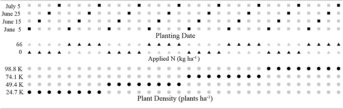
Table 1. The 32 management options modeled in the CERES-Sorghum simulations.

As in M19, distributions of dryland sorghum yield were formed for each of the 32 management options by aggregating simulated yields from every station's model runs over the years 2005–2010 and 2012–2016. As the 2011 drought year produced no dryland upland cotton over the Southern High Plains (Dever et al., 2012), that year's simulated sorghum yields were withheld to maintain consistency with M19. Thus, for each management option, CERES-Sorghum was run for 11 years with the weather inputs for each of Figure 1's 21 WTM stations, which produced 231 grain yield values. For each MO those values were ranked into percentiles (e.g., as in Figure 2) to form densely sampled grain yield distributions.

FIGURE 2

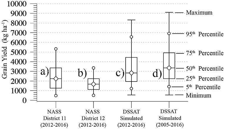
Figure 2. (a) Sorghum grain yield percentiles of aggregated NASS District 11 yield reports during the 2012–2016 cropping years. (b) As in (a) for NASS District 12 yield reports. (c) Grain yield percentiles of CERES-Sorghum simulations aggregated over 21 locations and 32 management options during 2012–2016 (3,360 yields). (d) As in (c) for modeled yields aggregated over the 11 years of 2005–2010 and 2012–2016 (7,392 yields).

Comparison of Modeled vs. NASS Production Yield Percentiles

The Figures 2a,b barplots plot percentiles of recent sorghum grain yields reported by producers in the U.S. National Agricultural Statistics Service's (NASS) Districts 11 and 12. The NASS Objective Yield Surveys for west Texas sorghum are based on between 100 and 300 yield reports each year (Lindsay Drunasky, personal communication), and the Figures 2a,b percentiles were estimated from yield reports aggregated over the 2012–2016 cropping years. Figure 2c plots the percentiles of 2012–2016 CERES-Sorghum simulated grain yields based on the Kothari et al. (2019) cultivar parameters. Those yields were generated from the 21 station's weather inputs during those 5 years over all of the 32 management options, which produced 3,360 simulated yields.

The medians and inter-quartile range (IQR) of District 12 yields (1,681 and 1,116 kg ha⁻¹,) are noticeably less than that of District 11 (2,239 and 2,107.4 kg ha⁻¹). A tendency for lower District 12 yields was also found in NASS dryland cotton yields in M19, which may be due to a combination of sandier soils, less rainfall and higher evapotranspiration in the more southern District 12 region. The Figure 2c simulated median yield (2,838 kg ha⁻¹) is almost 600 kg ha⁻¹ greater than that of the NASS District 11 median and 1157.1 kg ha⁻¹ greater than the NASS District 12 median (1,681 kg ha⁻¹). Higher modeled yields might be attributed to the simulations being based on one soil type and a range of initial soil moisture conditions higher than those that SHP sorghum producers might typically plant into. Figure 2d shows the percentiles of simulated yields aggregated over the 2005–2010 and 2012–2016 growing seasons and over all of the 32 management options (7,392 yields). The addition of the 2005–2010 simulated yields leads to a 522 kg ha⁻¹ increase in median yield relative to Figure 2c, and an increase of the IQR to 2,672 kg ha⁻¹.

Results

Simulated Grain Yields by Management Option

Figure 3a's barplot diagrams show the 32 yield distributions that result after Figure 2d's modeled yields have been separated by management option. A consistent repeating “sawtooth” pattern in median and 75th yield percentiles shows increased yields as planting dates are delayed from June 5th to July 5th. Plant density has a less obvious effect, with yield percentiles for the same planting data and N application gradually decreasing as density increases from 24.7 to 98.8 K plants ha⁻¹, e.g., compare the 75th yield percentiles for MO 4, 12, 20, and 28. An additional management effect is that of increased yield variability with later planting dates. For example, the spread between the 75th and 25th yield percentiles for MO 4, i.e., the inter-quartile range (IQR), is 3,078 kg ha⁻¹. By contrast, the IQR of MO 1—which differs from MO 4 by only by an earlier June 5 planting date—is 2,018 kg ha⁻¹. The management option producing the highest median (4,014 kg ha⁻¹) is MO 4, which plants on July 5th at the lowest plant density and applies no nitrogen. The lowest median yield (2,870 kg ha⁻¹) results from MO 29, which plants on the earliest of the 4 planting dates at the highest plant density and applies 66 kg ha⁻¹ N.

FIGURE 3

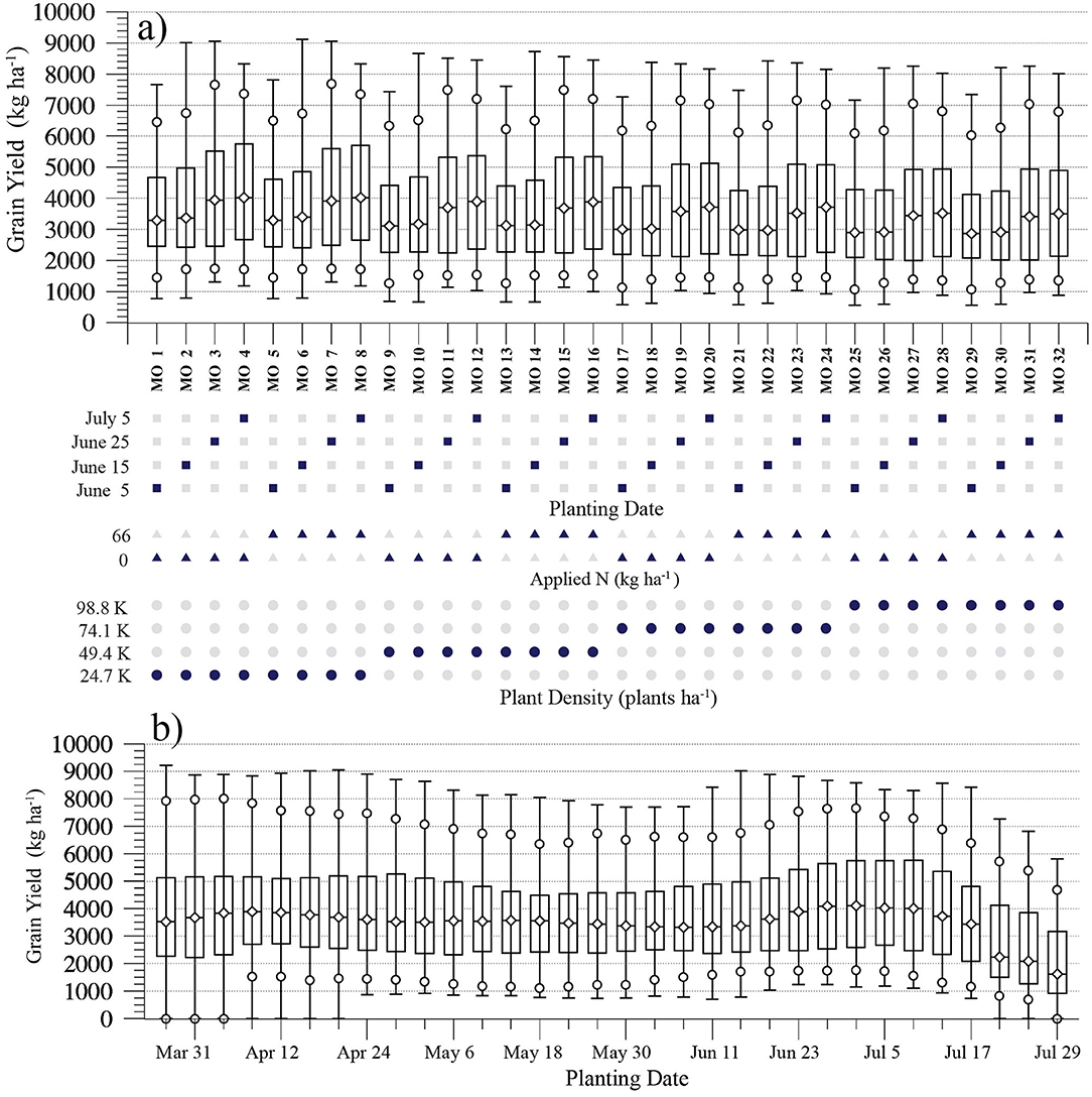
Figure 3. (a) Percentiles of simulated grain yields for Table 1's 32 management options, each aggregated over the 21 station's simulations during the 11 years of 2005–2010 and 2012–2016 (231 yields). (b) Percentiles of simulated grain yields for MO 4 plant density and applied N, for March 27th to July 29th planting dates at 4 day intervals.

To show planting date effects over a wider range of dates, Figure 3b's yield distribution's result from the MO 4 option's plant density and 0 kg ha⁻¹ applied N rate, but with March 27th to July 29th planting dates. Median simulated yields are relatively constant with planting dates before June 7th, increase to a maximum between June 27th and July 9th, and then decrease abruptly with later planting dates. Thus, Figure 3a's “sawtooth” yield effect with later planting is a consequence of simulated median yields peaking with late-June to early-July planting dates. The highest median (4,108 kg ha⁻¹) occurs with a July 1st planting date.

Figure 4 shows Figure 3a's yield distributions ordered by their median yields. Consistent with Figure 3a's sawtooth yield pattern, the 16 highest medians occur with either a June 25 or July 5th planting date. The 16 lowest medians occur with June 5 or June 15 planting dates. The management options producing the 4 highest median yields plant at the lowest plant density, while the 4 lowest medians result from options with the highest plant density. By contrast, there is no clear pattern of median yield effects associated with the two N levels.

FIGURE 4

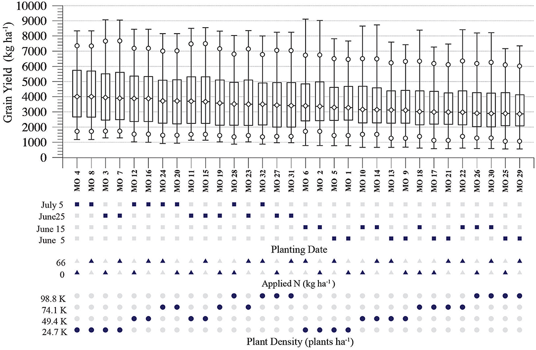
Figure 4. As in Figure 3a, with each management option's yield distribution plotted in order from the highest to the lowest median grain yield.

Management-Related Yield Effects

To isolate and compare the contributions of planting date, planting density, and applied N levels to MO 4 yields, Figure 5 shows yield effect (Δ_Y) distributions associated with selecting that option over alternate management practices. Yield effects for each station-year were calculated by subtracting yields resulting from an alternate practice from MO 4 yields, with the alternate yields simulated with the same station-year's initial soil moisture conditions and daily weather inputs. As yields from both management options were generated under the same initial and environmental conditions, the resulting Δ_Y value estimates a yield effect due to management. The resulting Δ_Y distributions might be used to estimate the probability of yield effects due to management choices under current climate conditions. Figure 5a shows the distribution of 231 yield effects resulting from selecting MO 4 over the management option producing the lowest median yield, i.e., MO 29. In addition to producing the highest and lowest median yields, these options also reflect management extremes, i.e., the latest vs. earliest planting date, lowest vs. highest plant density, and no vs. 66 kg ha⁻¹ applied N. As a result, the Figure 5a MO4–MO29 Δ_Y distribution estimates the range of potential yield effects due to the combined influence of planting date, planting density, and applied N. The MO 1 management option differs from MO 4 only by planting date, i.e., earliest vs. latest. Thus, the Figure 5b MO 4–MO 1 Δ_Y distribution estimates the exclusive yield effects of selecting a July 5th over a June 5th planting date (“PDATE-Only”). Similarly, Figure 5c's MO 4–MO 28 distribution shows the yield effects of plant density only (“PDENS-Only”), as MO 28 differs from MO 4 only in selecting the highest rather than lowest plant density. Figure 5d's MO 4–MO 8 “APPN-Only” distribution shows only fertilization effects, as those options differ only in the levels of applied N.

FIGURE 5

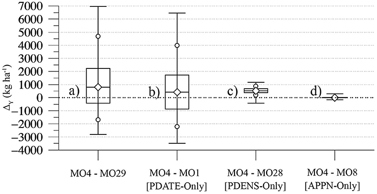
Figure 5. (a) Distribution of yield effect (Δ_Y) values resulting from subtracting grain yields generated via the MO 29 management option from the yield generated via the MO 4 option using the same station-year's weather data. (b) As in (a) for Δ_Y values generated by subtracting MO 1 from MO 4 yields. (c) As in (a) for Δ_Y values generated by subtracting MO 28 from MO 4 yields. (d) As in (a) for Δ_Y values generated by subtracting MO 8 from MO 4 yields.

In Figure 5a, the median MO 4–MO 29 yield effect is 798 kg ha⁻¹. However, 80 of the 231 Δ_Y values are negative, with values as large as −2,818 kg ha⁻¹. Thus, even though Figure 3a's MO 4 median yield is 1,144 kg ha⁻¹ greater than the MO 29 median, these simulations estimate a 34.6% probability that MO 4 would produce smaller yields in any given year under current SHP summer climate conditions. In Figures 5b,c the median PDATE-Only (421 kg ha⁻¹) yield effect is less than that of the median PDENS-Only effect (515 kg ha⁻¹), but the IQR of the former (2,610 kg ha¹) is almost 9 times larger than that of the latter (293 kg ha⁻¹). As a result, the simulations show considerably more yield variability in planting date effects than in planting density effects. The Figure 5b PDATE-Only distribution's range and IQR are similar to that of Figure 5a, which shows that the variability of MO 4–MO 29 yield effects is mainly a planting date effect. This also shows that the 34.6% probability of negative MO 4–MO 29 yield effects is due mainly to earlier planting dates, as the PDATE-Only distribution's median and wide dispersion leads to a 41.6% probability of a negative yield effect. However, given the roughly equivalent PDATE-Only and PDENS-Only median yield effects, planting date and planting density make roughly equal contributions in determining the location of the MO 4–MO 29 Δ_Y distribution. In Figure 5d, applied N yield effects are minor, with a median Δ_Y of 4 kg ha⁻¹ and 90% of effects occurring between −34 and 59 kg ha⁻¹.

Summary and Discussion

Of the 32 simulated sorghum management options (Table 1) the highest median grain yield was produced by the option that planted on the latest planting date (July 5th), at the lowest plant density (24.7 K plants ha⁻¹), and applied no nitrogen (MO 4). As in the M19 dryland cotton simulations, applied N had negligible yield effects that might be attributed to the background soil N content assumed in both studies. Although this 96 kg ha⁻¹ level is consistent with estimates of average SHP N levels (Bronson et al., 2009), it is high relative to the needs of sorghum for realistic dryland grain yields in the region. Thus, an additional 66 kg ha⁻¹ N application had minor effects on grain yields, which, given the input costs of applied N, would likely lead to reduced profits. Under production conditions this highlights the need for soil N testing before planting, as residual SHP soil N levels may be high enough to support dryland sorghum production.

The clearest management effect found was increased median yields as planting is delayed from June 5th to July 5th (Figure 3a). Over a wider range of planting dates the CERES-Sorghum simulations show that, under 2005–2016 SHP climate conditions, median yields are maximized with late-June to early July planting dates (Figure 3b). This yield effect is interpreted here as a consequence of, in effect, synchronizing a dryland sorghum crop's high-water demand growth phase to an SHP fall wet period. Figure 6 shows running 15-day rainfall totals averaged over Figure 1's 21 WTM stations during 2005–2016, with error bars marking ± 2σ uncertainty in the means. Following the growth cycle of a medium maturity sorghum cultivar (Gerik et al., 2003), the figure's crop development timeline marks a July 5 planting date, emergence after 7 days, and 3 consecutive 33-day periods of vegetative growth, reproductive growth, and grain filling. The May to September summer growing season coincides with the region's annual wet period, which is interrupted by relatively dry conditions during late July and early August. Wet conditions return in early Fall, with the wettest 15-day periods during 2005–2016 occurring during the first 2 weeks of September. Sorghum is most sensitive to water stress during the period between panicle initiation and flowering (Jones and Johnson, 1991; Gerik et al., 2003), which defines its reproductive growth stage. Late June to early July planting dates allow the SHP region's early September wet period to coincide with the crop's boot stage, which occurs during the latter portion of reproductive growth when the crop's water requirements are greatest (Gerik et al., 2003). As noted by Trostle et al. (2010), mid-summer planting dates also allow for higher soil moisture accumulation during the region's May–June wet period.

FIGURE 6

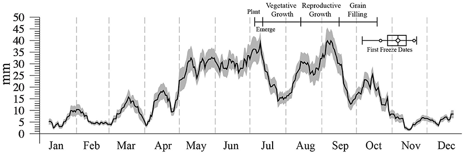
Figure 6. Black trace marks the average of running 15-day rainfall totals over Figure 1's 21 WTM stations during each year of 2005–2016 (n = 252). Gray error bars mark ± 2σ uncertainty in the means. Barplot shows the percentiles of first hard freeze dates (daily T_min < −2.2°C) for each of the 252 station-years. Crop development timeline marks growth phases for a medium maturity sorghum cultivar planted on July 5.

Although first freeze dates restrict how late SHP sorghum can be planted, late-June to early July planting dates are consistent with the latest dates (June 25–July 5) recommended by regional extension (Barber and Trostle, 2007) for medium maturity grain sorghum similar to that modeled here. Figure 6's barplot shows the percentiles of first freeze dates for the 21 WTM stations during 2005–2016, where first freeze is defined as the first fall day when daily minimum temperature falls below −2.2°C (28.0°F). The earliest of the 252 first freeze dates is October 6, with 50% of the dates occurring before Nov 10. Regional extension (Trostle et al., 2010) recommends that planting dates should allow for physiological grain maturity to occur 2–3 weeks before first freeze. An October 19 maturity date with a 3 week buffer period would require a first freeze later than November 9, which is 1 day before the November 10 median date for 2005–2016. Thus, there is a ~50% probability that the requirements for that buffer period would be met with a medium maturity cultivar planted on July 5. Increasing that probability might be achieved with late June planting, and/or a more rapidly maturing cultivar. However, a practice of late-planting sorghum may not be best for more northern SHP locations with earlier freeze dates. In the SORKAM simulations of Baumhardt et al. (2005), which were driven by long-term weather data from a UDSA-ARS research site at Bushland, TX (35° 11′N, 102° 5′ W), freezing fall temperatures prevented sorghum planted on June 25 from reaching physiological maturity. It should also be noted that late June or early July planting in the CERES-Sorghum simulations did not result in unconditionally increased yields. In a yield effect analysis that calculated differences in yield outcomes resulting from planting on July 5 and June 5, in 41.6% of the simulations June 5 planting produced higher yields (Figure 5b). Thus, under current climate conditions the estimated probability of early July planting leading to higher yields is 58.4%, only slightly better than that of an evenly-weighted coin flip.

The effect of the 32 management options on median yield (Figure 4) show that the 4 options with the highest median yields plant at a 24.7 K plants ha⁻¹ density. However, there is little supporting evidence that a density that low would maximize yields in other SHP field and modeling studies, and an optimal density for dryland conditions in uncertain. Based on field trials, Jones and Johnson (1991) estimated that dryland SHP sorghum yields would be maximized with a 59.3 K plants ha⁻¹ density, with densities between 39.5 and 83.9 K plants ha⁻¹ producing yield reductions of <5%. But although 24.7 K plants ha⁻¹ density is less than half that estimated to maximize yields in the Jones and Johnson (1991) field experiments, those trials were conducted over a 3-year (1986–1988) period with above average growing season rainfall during each year. As a result, their optimal plant density may not be representative of SHP summer climate conditions and dryland sorghum production. By contrast, the CERES-Sorghum simulations here were based on a more represent range of summer rainfall variability. However, CERES-Sorghum validation tests (White et al., 2015) have showed that the model did not perform well in attempts to reproduce population effects found in the Jones and Johnson (1991) experiments. As a result, whether the simulated optimal planting rate found here reflects actual dryland production conditions is open to question. In an irrigated field experiment conducted at Halfway, Texas (Trostle and Barber, 2008), nine seeding rates were tested that produced plant populations between 54.8 and 202.0 K plants ha¹, but no clear general trend between seeding rate and grain sorghum yields was found. Based on dryland SORKAM simulations that tested the effects of planting date, plant population (30.0, 60.0, and 120.0 K plants ha⁻¹), row spacing, and cultivar maturity, Baumhardt et al. (2005) found that the highest simulated plant population decreased panicle seed number, seed mass, and tiller number. Given lower yields with higher plant populations, they recommended either 30.0 or 60.0 K plants ha⁻¹ densities of early or medium maturing cultivars to achieve higher SHP dryland sorghum yields. These densities are generally consistent with current SHP extension guidelines for dryland production (Trostle et al., 2010), which recommend plant populations between 34.6 and 69.2 K plants ha⁻¹.

Determining an SHP dryland sorghum planting density that maximizes yield may require additional field studies of density effects, but conducted with lower densities more consistent with dryland production. Or, CERES-Sorghum could be modified to allow it to independently reproduce planting density effects found in the field. By contrast, the yield maximizing effect of late planting dates seen here is consistent with SHP summer rainfall climatology and sorghum's growth cycle. Mid-summer planting might also allow for longer periods of spring and early summer soil moisture accumulation. Thus, Figure 3b's late-June and early July increase in median yields is likely a consequence of the model's ability to translate soil moisture into yield. There is less need to confirm this management effect in the field, as the CERES-Sorghum growth parameters were validated based on the model's ability to reproduce the yield response to applied water in irrigated field studies (Kothari et al., 2019).

The results here and in M19 demonstrate a simulation-based method for identifying climate-optimized dryland management practices and estimating climate-related risk. This approach is based on the availability of a large sample of a growing region's seasonal weather outcomes, which were provided in both studies by West Texas mesonet station data (Schroeder et al., 2005) during 2005–2016. In growing regions where mesonet data is unavailable, weather generators might be used to simulate a dense meteorological network based on weather data from an existing lower resolution network (Wilks, 1999). Given large samples of observed or simulated seasonal weather data, a calibrated crop model is used to convert those weather outcomes into similarly sampled yield distributions. Best management practices for current climate can be sought by running the model over a range of management practices that are optimal under specific production goals. The best practices here were those that maximized median yields, but management options that minimize profit risk could also be identified. But, as noted above, model responses to management options should be verified against the results of field experiments. As shown in M19 and here, optimal practices for different dryland crops may be adaptations to different environmental factors. In M19 the mid-May planting dates that increased total growing degree days and maximized median cotton lint yields were basically a response to the SHP region's cool growing conditions. The CERES-Sorghum simulations here show that early July planting dates increase median sorghum yields by causing a crop's peak water-demand period to coincide with an early fall wet period. But in both cases, the dense yield distributions generated by this approach can be used to estimate the probability of dryland yield outcomes under a region's current climate conditions.

Yield variability is a leading driver of economic risk in semi-arid dryland agriculture, but variation in commodity prices and input costs also plays a role. In a final profit analysis, not conducted here but the goal of future work, the dense simulated yield distributions for dryland cotton and sorghum will be translated into corresponding profit distributions based on farm budgets appropriate to each crop. Given the resulting profit distributions, economic risk for each crop, e.g., the probability of operating costs exceeding yield revenues under specified commodity prices and input costs, can be calculated. In addition, the sensitivity of net returns to variation in commodity prices and input costs can be estimated. Given the leading influence of planting date found here and in M19, the effects of planting date on profit risk can be calculated. Also, the profitability of dryland cotton and sorghum under varying commodity prices can be compared.

Data Availability Statement

The datasets generated for this study are available on request to the corresponding author.

Author Contributions

SM ran the CERES-Sorghum model, led analysis of the simulated yield data, and wrote the first draft. GL assisted in running the CERES-Sorghum model. KK and SA provided model calibration coefficients and assisted in analysis of simulated yields. YE, ZX, and CH interpreted simulated yield results in the context of the sorghum growth cycle, past field research, and regional extension guidelines. RL interpreted the simulated yield results in the context of past Southern High Plains sorghum modeling studies. All authors assisted in writing and improving the paper's final draft.

Conflict of Interest

The authors declare that the research was conducted in the absence of any commercial or financial relationships that could be construed as a potential conflict of interest.

Acknowledgments

The authors would like to thank NOAA's National Mesonet Program and Texas Tech University for continued support in maintaining the West Texas Mesonet. Thanks to Lindsay Drunasky, Adam Wosoba, Jason Hardegree, and Wil Hundl of the National Agricultural Statistics Service for help in obtaining sorghum production data. All figures were produced using Generic Mapping Tools (Wessel et al., 2013). The mention of trade or manufacturer names is made for information only and does not imply an endorsement, recommendation, or exclusion by the USDA-Agricultural Research Service. The USDA is an equal opportunity provider and employer.

Abbreviations

WTM, West Texas Mesonet; SHP, Southern high plains.

References

Alagarswamy, G., and Ritchie, J. (1991). “Phasic development in CERES-Sorghum model,” in Predicting Crop Phenology, ed T. Hodges (Boca Raton, FL: CRC Press), 143–152.

Google Scholar

Amosson, S., Guerrero, B., and Graham, H. (2014). The Impact of the Feed Grains Industry in the Southern Ogallala Region. Available online at: https://www.agrilifebookstore.org/GrainsIndustry-on-the-Southern-Ogallala-Region-p/eag-011.htm (accessed September 12, 2018).

Barber, J., and Trostle, C. (2007). Recommended Last Planting Date for Grain Sorghum in the Texas South Plains - 2007. Lubbock, TX: Texas A&M AgriLife Research Center. Available online at: https://agrilifecdn.tamu.edu/lubbock/files/2011/10/lastrecsorgplantingdatetx07_71.pdf (accessed May 19, 2019).

Baumhardt, R. L., Tolk, J. A., and Winter, S. R. (2005). Seeding practices and cultivar maturity effects on simulated dryland grain sorghum yield. Agron. J. 97, 935–942. doi: 10.2134/agronj2004.0087

CrossRef Full Text | Google Scholar

Bordovsky, J., Keeling, W., Amerson, K. C., Hardin, C., and Cranmer, C. A. (2013). “Grain sorghum performance at multiple irrigation levels,” in Helm Research Farm Summary Report 2013, Texas A &M Agrilife Research Technical Report No. 14-4. Available online at: http://lubbock.tamu.edu/files/2014/04/Binder1.pdf (accessed August 18, 2018).

Bronson, K. R., Malapati, A., Booker, J. D., Scanlon, B. R., Hudnall, W. H., and Schubert, A. M. (2009). Residual soil nitrate in irrigated southern high plains cotton fields and Ogallala groundwater nitrate. J. Soil Water Conserv. 64, 98–104. doi: 10.2489/jswc.64.2.98

CrossRef Full Text | Google Scholar

Chapman, S. C., Cooper, M., Hammer, G. L., and Butler, D. G. (2000). Genotype by environment interactions affecting grain sorghum. II. Frequencies of different seasonal patterns of drought stress are related to location effects on hybrid yields. Austr. J. Agric. Res. 51, 209–222. doi: 10.1071/AR99021

CrossRef Full Text | Google Scholar

Dahlberg, J., Berenji, J., Sikora, V., and Latkovic, D. (2011). Assessing sorghum [Sorghum bicolor (L) Moench] germplasm for new traits: food, fuels and unique uses. Maydica 56, 85–92.

Google Scholar

Dever, J. K., Wheeler, T. A., Kelley, M. S., Kerns, D., Riley, M. E., Cranmer, A., et al. (2012). Cotton Performance Tests in the Texas High Plains and Trans Pecos Areas of Texas 2011. Texas A&M Agrilife Research Technical Report 12-2. Available online at: https://agrilife.org/lubbock/files/2012/01/2011CottonBooklet.pdf (accessed February 8, 2018).

Google Scholar

Evett, S. R., Howell, T. A., Schneider, A. D., Copeland, K. S., Dusek, D. A., Brauer, D. K., et al. (2015). The Bushland weighing lysimeters: a quarter century of crop ET investigations to advance sustainable irrigation. Trans. ASABE 59, 163–179. doi: 10.13031/trans.59.11159

CrossRef Full Text | Google Scholar

Gerik, T., Bean, B., and Vanderlip, R. (2003). Sorghum Growth and Development. Texas A&M University. Available online at: http://glasscock.agrilife.org/files/2015/05/Sorghum-Growth-and-Development.pdf (accessed November 20, 2018).

Google Scholar

Haacker, E. M. K., Kendall, A. D., and Hyndman, D. W. (2016). Water level declines in the High Plains aquifer: predevelopment to resource senescence. Groundwater 54, 231–242. doi: 10.1111/gwat.12350

PubMed Abstract | CrossRef Full Text | Google Scholar

Hammer, G. L. (2006). Pathways to prosperity: breaking the yield barrier in sorghum. Agric. Sci.19, 16–22.

Google Scholar

Hammer, G. L., McLean, G., Chapman, S., Zheng, B., Doherty, A., Harrison, M. T., et al. (2014). Crop design for specific adaptation in variable dryland production environments. Crop Pasture Sci. 65, 614–626. doi: 10.1071/CP14088

CrossRef Full Text | Google Scholar

Hoogenboom, G., Porter, C. H., Shelia, V., Boote, K. J., Singh, U., White, J. W., et al. (2017). Decision Support System for Agrotechnology Transfer (DSSAT) Version 4.7. Gainesville, FL: DSSAT Foundation. Available online at: https://DSSAT.net (accessed January 6, 2020).

Google Scholar

Jones, J. W., Hoogenboom, G., Porter, C. H., Boote, K. J., Batchelor, W. D., Hunt, L. A., et al. (2003). The DSSAT cropping system model. Eur. J. Agron. 18, 235–265. doi: 10.1016/S1161-0301(02)00107-7

CrossRef Full Text | Google Scholar

Jones, O. R., and Johnson, G. L. (1991). Row width and plant density effects on Texas High Plains sorghum. J. Prod. Agric. 4, 613–621. doi: 10.2134/jpa1991.0613

CrossRef Full Text | Google Scholar

Kothari, K., Ale, S., Bordovsky, J. P., Thorp, K. R., Porter, D. O., and Munster, C. L. (2019). Simulation of efficient irrigation management strategies for grain sorghum production over different climate variability classes. Agric. Syst. 170, 49–62. doi: 10.1016/j.agsy.2018.12.011

CrossRef Full Text | Google Scholar

Livezey, R. E., and Timofeyeva, M. M. (2008). The first decade of long-lead U.S. seasonal forecasts: Insights from a skill analysis. Br. Am. Meteorol. Soc. 89, 843–854. doi: 10.1175/2008BAMS2488.1

CrossRef Full Text | Google Scholar

Mauget, S., Adhikari, P., Leiker, G., Baumhardt, R. L., Thorp, K. R., and Ale, S. (2017). Modeling the effects of management and elevation on West Texas dryland cotton production. Agric. Forest. Meteorol. 247(Suppl. C), 385–398. doi: 10.1016/j.agrformet.2017.07.009

CrossRef Full Text | Google Scholar

Mauget, S., Marek, G., Adhikari, P., Leiker, G., Mahan, J., Payton, P., and Ale, S. (2019). Optimizing dryland crop management to regional climate via simulation. Part I: U.S. Southern High Plains cotton production. Front. Sustain. Food Syst. 3:120. doi: 10.3389/fsufs.2019.00120

CrossRef Full Text | Google Scholar

McGuire, V. L. (2017). Water-Level and Recoverable Water in Storage Changes, High Plains Aquifer, Predevelopment to 2015 and 2013–15. U.S. Geological Survey Scientific Investigations Report 2017–5040, 14. Available online at: https://pubs.usgs.gov/sir/2017/5040/sir20175040.pdf (accessed July 17, 2018).

Google Scholar

NASS (U. S. Department of Agriculture National Agricultural Statistics Service) (2019). Crop Production 2018 Summary. Available online at: https://www.nass.usda.gov/Publications/Todays_Reports/reports/cropan19.pdf (accessed July 2 2019).

Peng, P., Kumar, A., Halpert, M. S., and Barnston, A. G. (2012). An analysis of CPC's operational 0.5-month lead seasonal outlooks. Weather Forecast. 27, 898–917. doi: 10.1175/WAF-D-11-00143.1

CrossRef Full Text | Google Scholar

Schroeder, J. L., Burgett, W. S., Haynie, K. B., Sonmez, I., Skwira, G. D., Doggett, A. L., et al. (2005). The west Texas Mesonet: a technical overview. J. Atmos. Ocean. Tech. 22, 211–222. doi: 10.1175/JTECH-1690.1

CrossRef Full Text | Google Scholar

Sophocleous, M. (2010). Review: groundwater management practices, challenges, and innovations in the High Plains aquifer, USA, - lessons and recommended actions. Hydrogeol. J. 18, 559–575. doi: 10.1007/s10040-009-0540-1

CrossRef Full Text | Google Scholar

Trostle, C., and Barber, J. (2008). “Grain sorghum seeding rate on irrigated yield,” in Texas A&M AgriLife Helms Research Farm Summary Report 2008. Available online at: https://agrilifecdn.tamu.edu/lubbock/files/2012/04/2008helmsreport.pdf (accessed May 2, 2019).

Google Scholar

Trostle, C., Bean, B., Kenny, N., Isakeit, T., Porter, P., Parker, R., et al. (2010). United Sorghum Checkoff Program West Texas Production Guide, 2010. Available online at: http://www.sorghumcheckoff.com/assets/media/productionguides/2013_02WestTexasGuide.pdf (accessed May 19, 2019).

Wessel, W. H. F., Smith, R., Scharroo, J. F., Luis, and, F., and Wobbe (2013). Generic mapping tools: improved version released. EOS Trans. AGU 94, 409–410. doi: 10.1002/2013EO450001

CrossRef Full Text | Google Scholar

White, J. W., Alagarswamy, G., Ottman, M. J., Porter, C. H., Singh, U., and Hoogenboom, G. (2015). An overview of CERES-Sorghum as implemented in the cropping system model version 4.5. Agron. J. 107, 1987–2002. doi: 10.2134/agronj15.0102

CrossRef Full Text | Google Scholar

Wilks, D. (1999). Simultaneous stochastic simulation of daily precipitation, temperature and solar radiation at multiple sites in complex terrain. Agric. Forest. Meteorol. 96, 85–101. doi: 10.1016/S0168-1923(99)00037-4

CrossRef Full Text | Google Scholar