Optimizing Dryland Crop Management to Regional Climate via Simulation. Part I: U.S. Southern High Plains Cotton Production

Introduction

Although the Southern High Plains (SHP) of west Texas are home to some of the United States most concentrated upland cotton (Gossypium hirsutum L.) production, the region's environment is not ideally suited to growing cotton. Without irrigation, SHP summers are generally dry relative to conditions that maximize yield. During 1974–2005, the region's median May–Sept. rainfall was 29.2 cm (Mauget et al., 2013), which is less than half of the 74.0 cm estimated by Wanjura et al. (2002) to achieve maximum SHP lint yield. In addition, summer temperatures are generally considered to be cool relative to the requirements for cotton growth (Morrow and Kreig, 1990; Howell et al., 2004; Tolk and Howell, 2010). With enough soil moisture, SHP cotton lint yields are positively correlated with the cumulative exposure to daily average temperatures exceeding a base temperature during the summer growing season (Peng et al., 1989; Wanjura et al., 2002). For cotton, this threshold is typically 15.6°C (60.0 °F), and the resulting seasonal accumulations are referred to as growing degree days (GDD). Relative to the Rolling Plains region to the east, SHP cotton production areas are cooler due to the effects of higher elevation. As a result, the SHP accumulates fewer summer GDD, has generally later spring planting dates due to cooler soil temperatures, and has shorter summer growing seasons (Mauget et al., 2017; hereafter M17).

Cool growing conditions can reduce SHP cotton yields, but the most limiting factor in dryland production is summer rainfall. In addition, as in many other semi-arid agricultural regions, the unpredictable variation of growing season rainfall makes it difficult to manage SHP dryland crops. Although forecasts of growing season conditions issued before planting might allow producers to exploit wet summers or to insure against drought, there is currently little forecast skill for predicting U.S. summer precipitation (Livezey and Timofeyeva, 2008; Peng et al., 2012). Given the inability to forecast summer rainfall, Mauget et al. (2009) proposed the principle of “managing to climatology” (MtC), i.e., identifying and applying management practices for dryland crops that are adapted to a region's current climate conditions. In the context of the genetics X environment X management research framework (Hammer et al., 2014; Hatfield and Walthall, 2015) MtC might be understood as a simulation-based approach for optimizing crop management to a region's climate environment.

Because cotton yield variation is traceable in large part to water stress (Loka et al., 2011; Ullah et al., 2017; Khan et al., 2018), the timing and amount of growing season rainfall is the leading driver of yields in semi-arid dryland agriculture. As a result, identifying a climate-optimal management practice from a range of possible practices requires a broad sampling of seasonal rainfall outcomes and the resulting yields under each practice. If an additional goal is to estimate a practice's climate-associated risk with reasonable certainty, the sampling of rainfall variation and yield outcomes should be large and independent. Such yield ensembles could be produced through field trials, but generating large samples of dryland yields from multiple-year field experiments over a range of management options would require extensive labor, land, and financial resources. An alternative approach is to simulate dryland production with crop models. As in M17 and earlier work (Mauget et al., 2009, 2013), driving a crop model with weather inputs from numerous weather stations and then aggregating the resulting yields into distributions is a central feature of the MtC simulation approach used here. To broadly sample current summer rainfall outcomes over the SHP production region (Figure 1), weather inputs to the DSSAT CROPGRO-Cotton model were derived from 21 stations within Texas Tech University's West Texas Mesonet (WTM) network (Schroeder et al., 2005). Because of the spatial randomness of the SHP region's summer rainfall patterns, modeled yield outcomes derived from the weather inputs from this station network are roughly independent. Combining yields from summer growing seasons during 2005–2016 ensures that the resulting yield distributions are densely populated, but also representative of current SHP climate conditions. These yield distributions can be used to estimate the probability of dryland yield outcomes, and, if the corresponding profit for each yield is calculated, profit risk.

FIGURE 1

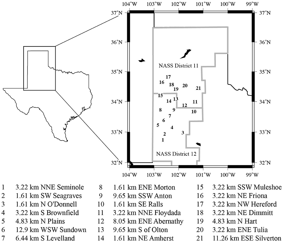
Figure 1. Locations of the 21 mesonet weather stations used to provide weather input data for the CROPGRO-Cotton model during 2005-2016.

Although crop modeling can be a useful tool for testing management options and estimating risk, agricultural production simulated by models is idealized. The simulated yields here, for example, are not affected by disease pressure, insect pressure, and the hail and wind events that frequently accompany spring rainfall in west Texas. Also, the CROPGRO-Cotton model does not simulate fiber quality characteristics that can determine lint value (Bradow and Davidonis, 2000; Delhom et al., 2018). On the other hand, crop simulation can expose management effects and climate-related risk that might not be apparent in field studies conducted over a limited number of years and/or locations. For example, past SHP field studies suggest that delayed planting in the region's cool growing environment can lead to reduced yields (Sansone et al., 2002; Woodward et al., 2013; Mauget et al., 2019). However, because these studies plant different cultivars on arbitrarily selected dates and produce small samples of yield outcomes, their results cannot provide controlled and accurate estimates of the risk associated with delayed planting. Although the goal of the M17 simulations was to isolate the effects of elevation on yield, they did not focus on the effects of management on yield over the important SHP cotton production region. The goal here is simulate higher elevation SHP dryland cotton production under conditions that are strictly controlled for non-climatic influences, e.g., yield variation due to management, cultivar, and soil type. Also, by conducting parallel simulations under identical initial soil moisture and weather conditions but different management practices, the simulated yields generated here can be used to estimate differential yield effects due to management (Δ_Y).

As a major U.S. agricultural area with substantial dryland production, limited summer rainfall, and dwindling ground water resources (Sophocleous, 2010; Steward et al., 2013; Haacker et al., 2016), the SHP might be considered a working laboratory for developing and applying methods in climate-related agricultural risk management. As in other semi-arid production regions there is a need to estimate the yield performance of dryland crops, define best management practices for those crops, and compare their profitability and production risk. To those ends, this paper is the first of two that explore climate-optimal practices in SHP dryland agriculture using the MtC modeling approach. This paper simulates dryland cotton production under a range of management practices, while a companion paper in this issue models dryland sorghum production. These two papers attempt to achieve three main goals: first, to describe and demonstrate a yield modeling framework for estimating climate-related risk in dryland agriculture; second, to define management practices for both crops that increase dryland yields in the current SHP environment; third, to generate databases of simulated dryland cotton and sorghum yields for subsequent work comparing the profitability of both crops.

In the following section Materials and Methods describes the CROPGRO-Cotton model and its calibration, the SHP weather records used to run the model, the procedure for assigning initial soil moisture in the model runs, and how the simulations were conducted. That section concludes by comparing CROPGRO-Cotton output statistics vs. recent regional dryland lint yield production statistics. Section Results presents the lint yield distributions of management options that result from all 32 possible combinations of 4 planting dates, 4 planting densities, and applying or not applying nitrogen. Section Discussion and Conclusions' discussion compares the section Results with that found in past field studies, and, given the simulated yield-increasing effects of mid-May planting, describes environmental conditions that might restrict SHP cotton planting.

Materials and Methods

The CROPGRO-Cotton Model

The cotton production model used here is CROPGRO-Cotton version 4.6.1.0 (Pathak et al., 2007, 2012), which is the cotton growth module of the Decision Support System for Agrotechnology Transfer (DSSAT) cropping system model (CSM: Jones et al., 2003; Hoogenboom et al., 2017). The DSSAT CSM consists of a group of software components that include growth modules that simulate the development of individual crops, and additional modules common to the growth simulation of a variety of crops. The latter include a main program, management module, soil module, weather module, and a soil-plant-atmosphere module. The management module controls operational conditions such as planting and harvesting date, irrigation scheduling when irrigation is simulated, the choice of evapotranspiration schemes, and residue and fertilizer applications. CROPGRO-Cotton requires inputs of environmental data, genetic information, and parameters defining crop management. Environmental data includes weather data, soil and soil profile characteristics, and potentially variable CO₂ levels. Here, CO₂ levels during 2005–2016 are assigned by DSSAT according to the monthly levels provided by Keeling et al. (2001). Although crop photosynthesis can be optionally calculated on an hourly basis, the model runs over daily time steps and requires daily weather data. For each plant growth module, cultivar, ecotype, and species coefficients are set in corresponding CUL, ECO, and SPE suffixed files that define genetic information. CROPGRO-Cotton calculates boll number, boll mass, seed cotton yield, and canopy height and width. The focus here is on lint yields derived from the model's seed cotton yield output. The model has been used to simulate cotton production over the SHP and nearby Texas Rolling Plains regions by Modala et al. (2015), Adhikari et al. (2016), and Mauget et al. (2017), and by Rahman et al. (2019) in Pakistan to simulate planting date and cultivar effects. A more in-depth overview of the DSSAT CSM and CROPGRO-Cotton can be found in Jones et al. (2003) and Thorp et al. (2014).

Model Calibration

The CROPGRO-Cotton cultivar and ecotype parameters used here were those estimated by Adhikari et al. (2016) based on 4 years of irrigated field trials (Bordovsky and Mustain, 2013) conducted at the Texas A&M AgriLife Research Center at Halfway (hereafter, “Halfway”). These trials were conducted using the FiberMax 9680B2RF cultivar, and during each year of 2010–2013 were repeated in 27 irrigation treatments defined by the application of low, medium, and high irrigation levels during three cotton growth periods. In Adhikari et al.'s (2016) calibration scheme the resulting 108 treatment outcomes over the 4-year period were divided into 16 calibration yields and 92 validation yields. CROPGRO-Cotton ecotype and cultivar parameters were adjusted to optimize the model's ability to reproduce the 16 calibration seed cotton yields, then the resulting FiberMax cultivar parameters were used in simulations to test the model's ability to independently predict the validation yields. That parameter set produced validation r² and average prediction error values of 0.94 and 6.5%, respectively, which indicates a reasonably high level of skill in predicting yield based on varying irrigation levels and a year's weather data inputs.

Weather Data Inputs

To generate distributions of seed cotton yield consistent with current SHP climate conditions, the CROPGRO-Cotton model was driven with daily weather inputs from 21 weather stations maintained by Texas Tech University's WTM network (Schroeder et al., 2005). Thirteen stations are located in the U.S. National Agricultural Statistics Service (NASS) District 12 production region, with the remaining 8 located in the neighboring NASS District 11 region to the north (Figure 1). These stations were selected from the WTM network based on their location in the two major west Texas cotton producing districts and their near-continuous meteorological records during Jan. 1 2005–Dec. 31 2016.

Although CROPGRO-Cotton requires daily weather inputs, WTM meteorological data is collected and reported every 5 min. Here, archived sub-daily records of minimum (T_min) and maximum temperature (T_max) at 2.0 m, dew point temperature (T_dew), precipitation (P), solar radiation (R_S), and 2.0 m wind speed (U₂) were averaged (T_min,T_max,T_dew), accumulated (P, R_S), or converted to a daily wind run value (U₂) over each day's 24 h. Soil temperatures (ST) at 10 cm depth are provided at 15-min intervals, and are averaged into daily values to estimate the probability of suitable spring planting conditions in section 5. The quality control (QC) procedures applied to the archived 5- and 15-min data records are described in Schroeder et al. (2005), while additional QC tests applied to the daily values calculated here are described in M17.

Initial Soil Moisture Conditions

Any attempt to model dryland cotton production in a semi-arid environment should account for all water sources, including initial soil moisture conditions. The procedure for assigning soil moisture content on each model run's first simulation day (Mar. 17) was based on neutron probe volumetric soil water content (SWC) measurements conducted at the ARS-Bushland weighing lysimeter facility (Evett et al., 2015). The Bushland large weighing lysimeters contain a Pullman Silty Clay Loam (Fine, mixed, superactive, thermic Torrertic Paleustoll) similar to the Pullman Clay Loam in which the Halfway 2010–2013 irrigated cotton trials were conducted. A Pullman Silty Clay Loam with soil water capacity, bulk density, and conductivity characteristics defined at 7 levels by the DSSAT SBuild utility was assumed in the CROPGRO-Cotton simulations. During 68 March, April, and May days in 1990, 1992, 1993, and 1997 the depth-weighted average percent of field capacity (%_FC) in the Bushland lysimeters ranged between 64.6 and 101.2%. Based on that range of spring soil moisture variability, the initial SWC over the depth of the model's soil profile was randomly assigned to be between 65 and 100% of field capacity. To ensure that simulations for each year and WTM station began with the same initial soil moisture conditions under various management options, initial SWC values for each station-year's crop simulation were defined with a unique random number generator seed equal to the sum of the station elevation and simulation year (2005–2016).

Dryland Cotton Simulations

Cotton simulations were repeated under 32 management options resulting from all possible combinations of 4 planting dates, 2 N applications, and 4 planting densities (Table 1). The latest planting date (June 5) is the last date that producers can plant and maintain eligibility for crop insurance in most District 12 counties. The earlier 3 dates were defined at 7-day intervals based on a sensitivity study described in Section 4. The background soil nitrogen level in the simulations was set equal to the regional average of 96 kg ha⁻¹ estimated from the soil N surveys conducted by Bronson et al. (2009). Given the typically low N levels applied in dryland cotton production and the high levels found in some SHP soils, simulations were repeated with no applied N, and 30 kg ha⁻¹ evenly divided between applications at planting and 50 days after planting. The simulations assumed a 76 cm row separation with 3,7,10, and 13 plants m⁻¹ plant separations, which approximately span those of the Stapper et al. (2011) field experiment (5.4, 10.1, and 12.9 plants m⁻¹).

TABLE 1

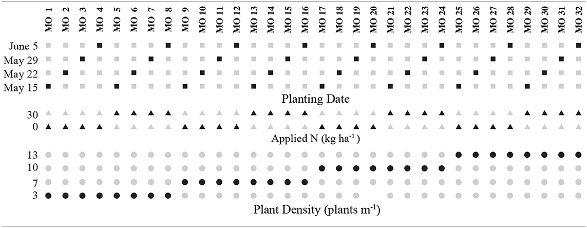
Table 1. The 32 management options modeled in the CROPGRO-Cotton simulations.

For each of the 32 management options (MO), distributions of cotton lint yield were generated by CROPGRO-Cotton driven by the WTM mesonet weather inputs. Each distribution was formed by running the model with daily weather inputs from Figure 1's WTM mesonet weather stations during 2005–2016, and then aggregating the yields resulting from the 21 station's model runs. Additional description of the process whereby DSSAT models generate yield outcomes based on weather data and other soil-plant-atmosphere interactions can be found in Jones et al. (2003). The unprecedented hot and dry conditions of 2011 over west Texas (Hoerling et al., 2013) resulted in essentially no SHP dryland cotton production (Dever et al., 2012), thus the model was not run based on that year's weather inputs. As a result, for each MO, the model was run based on each of the 21 station's weather inputs during 2005–2010 and 2012–2016, resulting in 21*11 = 231 simulated seed cotton yields. Lint yields were calculated from the CROPGRO-Cotton model's seed cotton output assuming a fixed seed to lint ratio. This ratio was set to 1.559, which is the average of the ratios of seven FiberMax cultivars reported during the 2016 Halfway cotton performance tests (Dever et al., 2017). Thus, each kilogram of the model's seed cotton yield is assumed to consist of 60.9% seed and 39.1% lint. The resulting 231 lint yields for a MO were ranked into percentiles to form densely sampled lint yield distributions consistent with current SHP dryland production conditions.

Model Validation vs. NASS Production Records

Figure 2 compares lint yield distributions of recent SHP dryland cotton production with the distribution of CROPGRO-Cotton modeled yields simulated over the same period based on the Adhikari et al. (2016) genetic parameters. Figure 2A show the percentiles of dryland upland cotton lint yields (kg ha⁻¹) derived from NASS District 11 yield surveys during 2012–2016. Figure 2B shows the same period's yield percentiles for NASS District 12. Although, NASS does not release survey yield counts, each district's survey during those 5 years is based on between 100 and 600 yield reports (Lindsay Drunasky, personal communication). To generate a concurrently modeled yield distribution for a range of management practices, CROPGRO-Cotton yields were aggregated over all 21 stations and all 32 management options in the 2012–2016 simulations (Figure 2C).

FIGURE 2

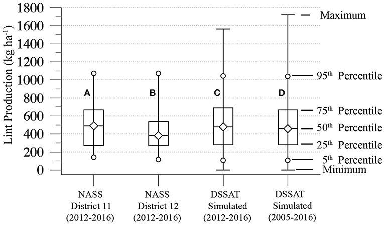
Figure 2. (A) Percentiles of lint yields derived from NASS District 11 un-irrigated yield reports during the 2012–2016 cropping years. (B) As in (A) for NASS District 12 yield reports. (C) Percentiles of modeled lint yields aggregated from CROPGRO-Cotton simulations conducted at 21 locations and 32 management options during 2012–2016 (21*32*5 = 3,360 yields). (D) As in (C) for modeled yields aggregated over the 11 years of 2005–2010 and 2012–2016 (21*32*11 = 7,392 yields).

The median of Figure 2C's 3,360 simulated lint yields (479.9 kg ha⁻¹) is 96.9 kg ha⁻¹ higher than the District 12 median (383.0 kg ha⁻¹), and 10.7 kg ha⁻¹ below the District 11 median (490.6 kg ha⁻¹). The simulated yield's 407.3 kg ha⁻¹ inter-quartile range (IQR), i.e., the 75th minus 25th percentile span, is only slightly greater than that of District 11 (395.4 kg ha⁻¹) but exceeds the District 12 IQR (268.8 kg ha⁻¹). The tails of both NASS yield distributions, as measured by the 5th and 95th percentiles, are shifted slightly above the 2012–2016 simulated yields. The lower District 12 median yield relative to that of District 11 might be attributed to the more southern region's generally sandier soils (Holliday, 1990) and higher evapotranspiration. Otherwise, the location and scale of Figure 2C's modeled yield distribution is closely consistent with the NASS District 11 distribution. This shows that, when initialized with realistic soil moisture conditions and driven by the WTM weather inputs, the calibrated CROPGRO-Cotton model can generate dryland lint yields that are representative of more northern SHP production areas under current summer climate conditions. When CROPGRO-Cotton lint yields for all 32 management options are aggregated over the 11 years of 2005–2010 and 2012–2016 (Figure 2D), the resulting yield percentiles are, apart from a greater maximum lint yield, generally similar to those of 2012–2016 in Figure 2C.

Results

Figure 3 shows the modeled lint yield percentiles that result when the Figure 2D distribution's yields are separated by management option, and each option's 231 yields are then ranked into percentiles. The clearest yield variation is that of a “descending sawtooth” effect, with later planting dates and higher plant densities producing generally lower median yields. Figure 4 shows the Figure 3 distributions ordered by median yield. This ordering is consistent with the Figure 3 planting date effect, with the earliest planting date producing 6 of the 7 highest medians and the latest date producing the 5 lowest medians. In addition, there is a somewhat weaker plant density effect, with 3 of the 4 highest median yields generated by simulations with the lowest planting density. The distribution with the highest median yield (MO 1) occurs with the May 15 planting date, the lowest the lowest plant density (3 plants per m⁻¹), and no applied N. By contrast, the MO32 option with the latest planting date (June 5), the highest plant density (13 plants m⁻¹), and 30 kg ha⁻¹ of applied N produces the lowest median yield.

FIGURE 3

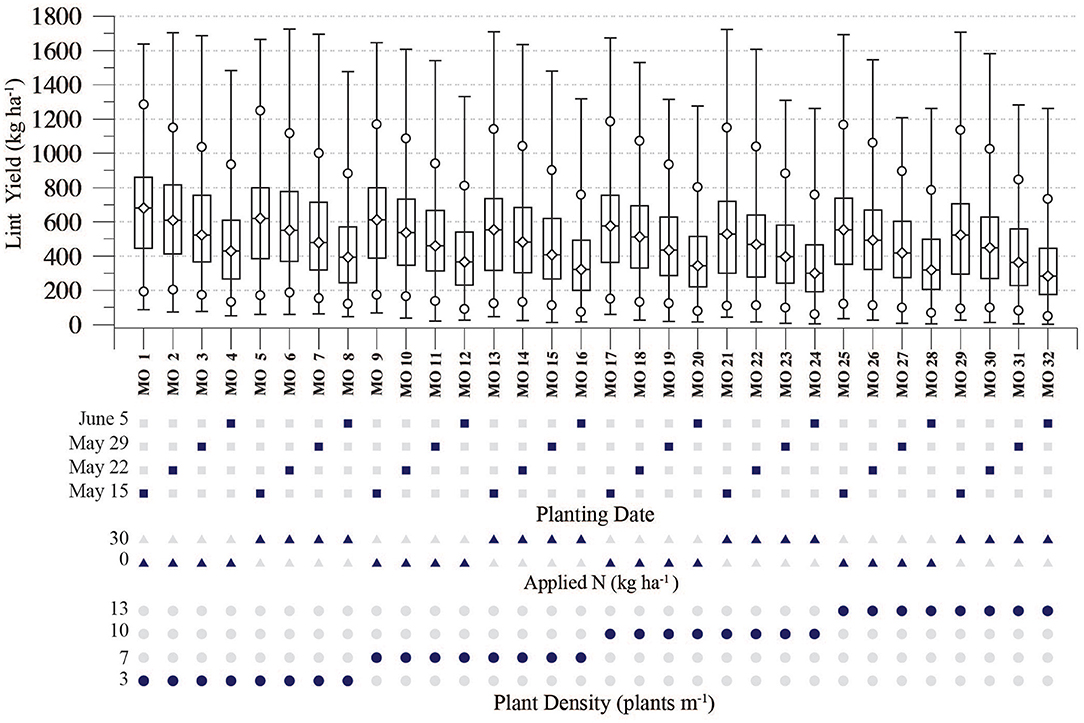
Figure 3. Percentiles of simulated lint yields for each of the 32 management options, each aggregated over the 21 station's simulations during the 11 years of 2005–2010 and 2012–2016 (21*11 = 231 yields).

FIGURE 4

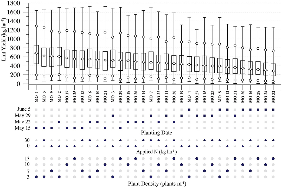
Figure 4. As in Figure 3, with distributions for each management option plotted in order from the highest to the lowest median lint yield.

The Figure 5A MO 1–MO 32 distribution shows the percentiles of lint yield effects (Δ_Y) resulting from choosing the MO 1 option over the MO 32 option. Thus for each of the 231 lint yields in the MO 1 distribution, a potential management effect, i.e., a “best minus worst” Δ_Y effect, is calculated by subtracting the corresponding MO 32 yield generated by the weather data from the same WTM station and the same year. The Figure 5B Δ_Y distribution estimates the exclusive effect of planting date (“PDATE-Only”) on the MO 1-MO 32 yield effects. As the MO 4 management option is effectively the MO 1 option with the MO 32 planting date (Table 1), these yield effects are calculated by subtracting MO 4 yields from the same station-year's yield outcomes in the MO 1 distribution, i.e., MO 1-MO 4. Similarly, the Figure 5C MO 1-MO 25 distribution estimates the effect of planting at a 3 vs. 13 plants per m⁻¹ plant density (“PDENS-Only”). Finally, the Figure 5D MO 1-MO 5 Δ_Y distribution estimates the impact of the two applied N levels on the MO 1-MO 32 lint yield differences (“APPN-Only”). Thus, Δ_Y values reflecting only N-based effects were calculated by subtracting modeled yields resulting from the MO 5 simulations (30 kg ha⁻¹) from the same station-year's MO 1 yields (0 kg ha⁻¹).

FIGURE 5

Figure 5. (A) Distribution of yield effect (Δ_Y) values resulting from subtracting lint yields generated via the MO32 management option from the lint yield generated via the MO1 option using the same station-year's weather data. (B) As in (A) for Δ_Y values generated by subtracting MO4 from MO1 yields. (C) As in (A) for Δ_Y values generated by subtracting MO25 from MO1 yields. (D) As in (A) for Δ_Y values generated by subtracting MO5 from MO1 yields.

Figure 5's four Δ_Y distributions show that planting date and plant density are the leading factors in the MO1-MO32 yield effects. The median MO 1-MO 32 Δ_Y value is 354.4 kg ha⁻¹, while the medians of the PDATE-Only, PDENS-Only, and APPN-Only distributions are 211.0, 107.1, and 42.2 kg ha⁻¹, respectively. The median PDATE-Only effect is 43% of the NASS district 11 median lint yield in Figure 2B (490.6 kg ha⁻¹), which suggests that delaying planting from mid-May to early-June can have a substantial negative effect on SHP dryland cotton yields. However, although 205 PDATE-Only Δ_Y values in Figure 5B are positive, 26 are negative, with yield effects as large as −290.3 kg ha⁻¹. Thus, while these simulations indicate a general yield advantages with mid-May planting, they also estimate an 11.3% probability that a June 5, rather than a May 15, planting date may produce higher yields under current SHP climate conditions.

Discussion and Conclusions

Although the highest median lint yields simulated here tend to occur at the lowest plant density (Figure 4), and lower density produced higher yields in more than 90% of Figure 5C's MO 1-MO 25 comparisons, past SHP field studies that test for plant density effects on yield are either inconclusive or suggest insignificant effects. A 2-year field study conducted by Bednarz et al. (2000) found that seed cotton yields were not influenced by population density. Their literature review, and that of Musunuru (2003), also notes a number of previous field trials indicating that cotton yields appear relatively stable over a range of plant densities. Woodward et al.'s (2013) focus was on disease incidence and fiber quality effects, and yield impacts due to seeding density were not reported. The Stapper et al. (2011) dryland trials found statistically insignificant yield outcomes with three seeding densities. During 2016 and 2017 Kimura and Ramirez (2018) planted at four seeding rates in irrigated and dryland Rolling Plains field trials, but also found no significant differences in lint yield. However, given effectively equivalent yield outcomes and the lower input costs of lower seeding rates, their lowest seeding density (54.9 K seeds ha⁻¹) did result in a positive and statistically significant profit effect.

The MO 1–MO 5 yield effects in Figure 5D showed that applying no N led to minor positive median yield effect relative to a management option that applied 30 kg ha⁻¹. Although counter-intuitive, this response may be due to the background soil N levels assumed here, which are high relative to the requirements of dryland cotton. The Hons et al. (2004) field trials found a significant response to additional applied N in only 8 of 39 trials during 1998–2002, which was attributed to already high residual soil N levels. A general rule of thumb in SHP production is to apply 28 kg ha⁻¹ (25 lbs acre⁻¹) of N for every 269 kg ha⁻¹ of anticipated lint yield (Hons et al., 2004). Current NASS production statistics show that 75% of dryland District 11 yields are under 667 kg ha⁻¹ (Figure 2B), which would require 69 kg ha⁻¹ of total soil and applied N. This dryland N requirement is well under of the 96 kg ha⁻¹ soil N level assumed here based on the Bronson et al. (2009) soil survey. As increasing total available N beyond that level in the simulations reduces yields, this, and the results of the Hons et al. (2004) trials, suggests that residual SHP soil N levels may be enough to achieve realistic dryland lint yield targets.

Unlike the modeled plant density effect, the leading effect of planting date on yield found here is consistent with that found in SHP field studies. To compare the CROPGRO-Cotton lint yield response to planting date with that found in a recent SHP field trial, Figure 6A shows distributions of yields generated to show MO 1 sensitivity to 32 planting dates at two-day intervals between April 4 and June 5. Thus, apart from planting date, the simulations were conducted with the MO 1 planting density and applied N level in Table 1. Simulations with planting dates before April 22 produce approximately stable yield percentiles, with at least 5% of the simulations in each failing to produce any yield. Although 5th percentiles are roughly constant between April 24 and June 5, the distribution's 95th percentiles decrease, with an increased rate of decline after mid-May. A similar pattern of decreased yields with planting dates after late April is seen in the distribution's medians, 25th, and 75th percentiles. Between May 14 and June 5 the simulated median lint yields decrease nearly linearly, with a linear-fit slope dropping 11.76 kg ha⁻¹ with every day's delay in planting.

FIGURE 6

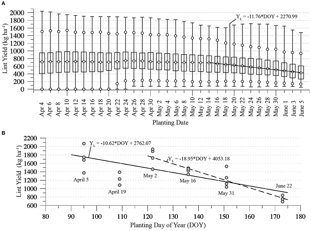
Figure 6. (A) Percentiles of simulated lint yields for 3 plants met⁻¹ plant density and 0 kg ha⁻¹ applied N, for planting dates between April 4 and June 5 at 2 day intervals. (B) Lint yields resulting from six planting dates during the PSWCL17 field trials. Dashed line plots linear fit to the May 2, 16, 31, and June 22 planted yields. Solid line plots a linear fit to the yields from all six dates.

Figure 6B graphs lint yields from 2017 field trials conducted at the USDA-ARS Plant Stress and Water Conservation Laboratory in Lubbock (hereafter PSWCL17), which included replications at four irrigation levels, each repeated at 6 planting dates between April 5 and June 22. The yields resulting from the May 2, 16, 31, and June 22 plantings generally decrease, with a linear-fitted slope estimating a 18.95 kg ha⁻¹ drop with every day's delay in planting. When yields planted on April 5 and 19 are included the linear-fit slope decreases to −10.62 kg ha⁻¹. Although the −18.95 kg ha⁻¹ PSWCL17 irrigated field trial response during May 2–June 22 is stronger than the −11.76 kg ha⁻¹ dryland CROPGRO-Cotton response, a stronger irrigated response is consistent with stronger GDD-related yield effects under lower water-stress conditions (Peng et al., 1989; Wanjura et al., 2002).

Generally, the PSWCL17 and other SHP field trials confirm the modeled yield effect of decreasing yields with delayed planting. Based on a 5-year field trial that planted on five dates between April 20 and June 30th, Bilbro and Ray (1973) found that later planting reduced yields, lint percentages, fiber length, and micronaire units, but increased fiber strength. Sansone et al. (2002) summarize the results of Lubbock area irrigated planting date trials during 1960–1966 that found a 24% decrease in average lint yield as planting was delayed from May 15 to June 10. Lower yields with April 22, May 12, and June 8 planting dates have also been found in Woodward et al.'s (2013) field trial exploring the effects of planting date, seeding density and cultivar. Mauget et al.'s (2019) analysis of yields in SHP May- and June-planted irrigated cultivar trials during 2007–2017 also found that May planting led to a significant positive average yield effect in 8 of 10 years that comparisons could be made.

The cause of the SHP planting date effect found here and in field studies is essentially geographic. Because of the region's elevation and cooler temperatures, its summer cotton growing season tends to be shorter and degree-day limited relative to neighboring regions at lower elevations (Mauget et al., 2017). As a result, earlier SHP planting dates tend to result in thermally longer growing seasons, higher GDD totals, and, given the positive association between GDD totals and SHP lint yield (Peng et al., 1989; Wanjura et al., 2002), higher yields. Thus, consistent modeling and field trial results demonstrate that early planting in the SHP's cooler growing environment might increase accumulated degree-days, crop growth, and yields. Although the focus here was on dryland cotton production, earlier planting may have an even greater effect on irrigated crops, given the greater effects of seasonal GDD accumulation on crops with lower levels of water stress. Mauget et al.'s (2019) analysis of 10 years of irrigated cultivar trials found that May-planted yields exceeded June-planted yields in 120 of 153 comparisons. The median yield effect in these comparisons was 371.7 kg ha⁻¹, which is considerably higher than the 211.0 kg ha⁻¹ median dryland effect of selecting a mid-May over an early-June planting date found here (Figure 5B). As a result, the primary conclusion of this modeling study is that planting date may be a key factor in adapting management to the SHP environment. Specifically, planting as early as conditions permit—with the mid-May period as a general management target—may be a relatively simple and cost-free management approach to increasing the region's dryland and irrigated cotton yields.

But although mid-May planting may result in thermally longer growing seasons and higher yields, the same cool conditions that produce shorter SHP growing seasons can also restrict when planting can occur. In addition to adequate soil moisture, soil temperatures before and weather conditions after planting are two important factors that determine when dryland cotton can be planted. The Figure 7 diamond-marked trace plots Figure 6A's simulated median lint yield values, which show a nearly linear decrease between May 14 and June 5. Planting on the former rather than the latter date in the simulations results in a 38% median yield increase from 430 to 690 kg ha⁻¹. Sansone et al. (2002) recommend that minimum daily soil temperatures at seed depth in the 3 day's before planting (ST₃₋) exceed 18.3°C (65.0 °F), and that average forecast daily temperatures result in a cotton growing degree day total in the 5 days after planting (GDD₅₊) >13.9°C (25.0 °F). Figure 7 also shows estimates of the probabilities of those two conditions being met over the Figure 1 WTM station network during the April 4–June 5 periods of 2005–2010 and 2012–2016. Thus, for each of the 32 planting dates, ST₃₋ and GDD₅₊ values were calculated from the 21 station records during those 11 years. The triangles plot the percentage of each date's 231 station-days when ST₃₋ > 18.3°C, the squares the percentage when GDD₅₊ > 13.9°C. If these percentages are interpreted as the probabilities of these conditions being met under current SHP climate conditions, between May 12 and May 18 the probability that GDD₅₊ exceeds 13.9°C rises from 41.6 to 90.0%. However, during this time the probability of ST₃₋ above 18.3°C at the 21 mesonet sites was no higher than 22.0%. Thus, while SHP temperature conditions above ground might allow for mid-May planting, an 18.3°C soil temperature requirement is likely to delay planting. Sansone et al. (2002) also propose that with a favorable GDD₅₊ forecast planting might occur in cooler soils, i.e., the ST₃₋ threshold might be lowered to 15.6°C (60.0 °F). The probabilities of this lower soil temperature condition being met generally track those of GDD₅₊ > 13.9°C in Figure 7. In mid-May under current SHP climate conditions, these GDD₅₊ and ST₃₋ conditions are met with an approximate 70% probability. As a result, the mid-May planting strategy proposed here may be more possible with the lower 15.6°C soil temperature threshold. However, planting low-vigor seed with lower germination rates into cooler soils can delay emergence, which has been found to reduce yields in SHP field trials (Wanjura et al., 1969). Thus, an SHP mid-May planting strategy may also require high vigor seed with higher emergence rates under cool soil conditions (Smith and Varvil, 1984).

FIGURE 7

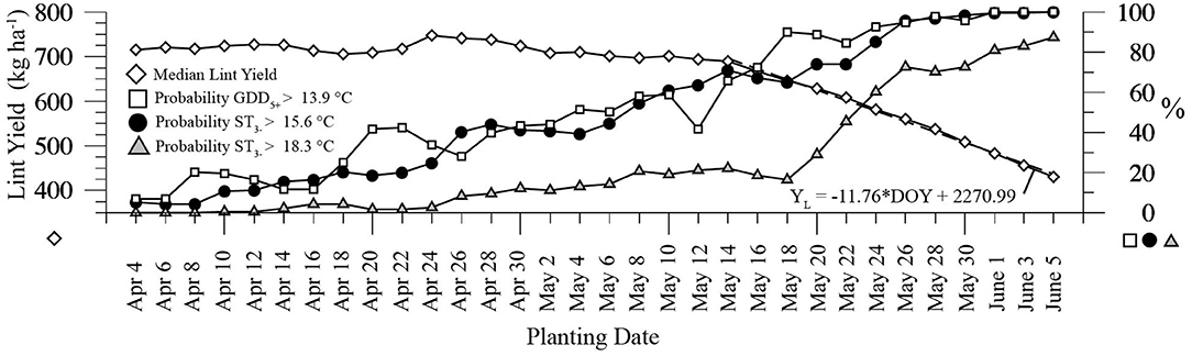
Figure 7. Diamonds mark the medians of the Figure 6A lint yield distributions. Gray triangles show the probability that minimum daily soil temperatures at 10 cm in the 3 days before each planting date (ST₃₋) exceeds 18.3°C. Black circles show similar probabilities based on a 15.6°C ST₃₋ threshold. Squares show the probability that cotton growing degree totals over the 5 day period after each planting date (GDD₅₊) exceeds 13.9°C.

Data Availability Statement

The datasets generated for this study are available on request to the corresponding author.

Author Contributions

SM ran the CROPGRO-Cotton model, led analysis of the simulated yield data, and wrote the first draft. GL assisted in running the CROPGRO-Cotton model. PA and SA provided model calibration coefficients and assisted in analysis of simulated cotton yields. JM and PP conducted the PSWCL17 field studies to estimate the effects of planting date on cotton yields and provided data. GM provided lysimeter-derived soil moisture data and assisted in estimation of initial soil moisture conditions. All authors assisted in writing and improving the paper's final draft.

Conflict of Interest

The authors declare that the research was conducted in the absence of any commercial or financial relationships that could be construed as a potential conflict of interest.

Acknowledgments

The authors would like to thank NOAA's National Mesonet Program and Texas Tech University for continued support in maintaining the West Texas Mesonet. Thanks to Lindsay Drunasky, Adam Wosoba, Jason Hardegree, and Wil Hundl of the National Agricultural Statistics Service for help in obtaining cotton production data. All figures were produced using Generic Mapping Tools (Wessel et al., 2013). The mention of trade or manufacturer names is made for information only and does not imply an endorsement, recommendation, or exclusion by the USDA-Agricultural Research Service. This research did not receive any specific grant from funding agencies in the public, commercial, or not-for-profit sectors. The USDA is an equal opportunity provider and employer.

Abbreviations

WTM, West Texas Mesonet; SHP, Southern High Plains; MtC, Managing to Climatology; DSSAT, Decision Support System for Agrotechnology Transfer.

References

Adhikari, P., Ale, S., Borodovsky, J. P., Thorp, K. R., Modala, N. R., Rajan, N., et al. (2016). Simulating future climate change impacts on seed cotton yield in the Texas High Plains using the CSM-CROPGRO-Cotton model. Agr. Water Manage. 164, 317–330. doi: 10.1016/j.agwat.2015.10.011

CrossRef Full Text | Google Scholar

Bednarz, C. W., Bridges, D. C., and Bloom, S. M. (2000). Analysis of cotton yield stability across population densities. Agron. J. 92, 128–135. doi: 10.2134/agronj2000.921128x

CrossRef Full Text | Google Scholar

Bilbro, J. D., and Ray, L. L. (1973). Effect of planting date on the yield and fiber properties of three cotton cultivars. Agron. J. 65, 606–609. doi: 10.2134/agronj1973.00021962006500040023x

CrossRef Full Text | Google Scholar

Bordovsky, J., and Mustain, J. (2013). Evaluation of Zero-Early Cotton Irrigation Strategy. Helm Research Farm Summary Report 2013, Texas A&M Agrilife Research Technical Report No. 14-4. Available online at: http://lubbock.tamu.edu/files/2014/04/Binder1.pdf (accessed August 18, 2016).

Google Scholar

Bradow, J. M., and Davidonis, D. H. (2000). Quantitation of fiber quality and the cotton production-processing interface: a physiologist's perspective. J. Cotton Sci. 4, 34–64.

Google Scholar

Bronson, K. R., Malapati, A., Booker, J. D., Scanlon, B. R., Hudnall, W. H., and Schubert, A. M. (2009). Residual soil nitrate in irrigated Southern High Plains cotton fields and Ogallala groundwater nitrate. J. Soil Water Conserv. 64, 98–104. doi: 10.2489/jswc.64.2.98

CrossRef Full Text | Google Scholar

Delhom, C. D., Kelly, B., and Martin, V. (2018). “Physical properties of cotton fiber and their measurement,” in Cotton Fiber: Physics, Chemistry and Biology, ed. D. Fang (Basel: Springer Nature), 41–73. doi: 10.1007/978-3-030-00871-0_3

CrossRef Full Text | Google Scholar

Dever, J. K., Morgan, V., Kelly, C. M., Wheeler, T. A., Byrd, S., Stair, K., et al. (2017). Cotton Performance Tests in the Texas High Plains 2016. Texas A&M Agrilife Research Technical Report 17-1, 45. Available online at: http://agrilife.org/lubbock/files/2017/02/Cotton-Book-online.pdf (accessed February 6, 2018).

Google Scholar

Dever, J. K., Wheeler, T. A., Kelley, M. S., Kerns, D., Riley, M. E., Cranmer, A., et al. (2012). Cotton Performance Tests in the Texas High Plains and Trans Pecos Areas of Texas 2011. Texas A&M Agrilife Research Technical Report 12-2, 62. Available online at: agrilife.org/lubbock/files/2012/01/2011CottonBooklet.pdf (accessed February 8, 2018).

Google Scholar

Evett, S. R., Howell, T. A., Schneider, A. D., Copeland, K. S., Dusek, D. A., Brauer, D. K., et al. (2015). The Bushland weighing lysimeters: a quarter century of crop ET investigations to advance sustainable irrigation. Trans. ASABE. 59, 163–179. doi: 10.13031/trans.59.11159

CrossRef Full Text | Google Scholar

Haacker, E. M. K., Kendall, A. D., and Hyndman, D. W. (2016). Water level declines in the High Plains aquifer: predevelopment to resource senescence. Groundwater 54, 231–242. doi: 10.1111/gwat.12350

PubMed Abstract | CrossRef Full Text | Google Scholar

Hammer, G. L., McLean, G., Chapman, S., Zheng, B., Doherty, A., Harrison, M. T., et al. (2014). Crop design for specific adaptation in variable dryland production environments. Crop Pasture Sci. 65, 614–626. doi: 10.1071/CP14088

CrossRef Full Text | Google Scholar

Hatfield, J. L., and Walthall, C. L. (2015). Meeting global food needs: realizing the potential via genetics X environment X management interactions. Agron. J. 107, 1215–1226. doi: 10.2134/agronj15.0076

CrossRef Full Text | Google Scholar

Hoerling, M., Kumar, A., Randall, D., Nielsen-Gammon, J. W., Eischeid, J., Perlwitz, J., et al. (2013). Anatomy of an extreme event. J. Clim. 26, 2811–2832. doi: 10.1175/JCLI-D-12-00270.1

CrossRef Full Text | Google Scholar

Holliday, V. T. (1990). Soils and landscape evolution of eolian plains: the Southern High Plains of Texas and New Mexico. Geomorphology 3, 489–515. doi: 10.1016/0169-555X(90)90018-L

CrossRef Full Text | Google Scholar

Hons, F. M., McFarland, M. L., Lemon, R. G., Nichols, R. L., Boman, R. K., Saladino, V. A., et al. (2004). Managing Nitrogen Fertilization in cotton. Texas A&M AgriLife Extention L-5458, 4. Available online at: https://agrilifecdn.tamu.edu/lubbock/files/2011/10/managingnfinc.pdf (accessed May 29, 2018).

Google Scholar

Hoogenboom, G., Porter, C. H., Shelia, V., Boote, K. J., Singh, U., White, J. W., et al. (2017). Decision Support System for Agrotechnology Transfer (DSSAT) Version 4.7. Gainesville, FL: DSSAT Foundation. Available online at: https://DSSAT.net (accessed January 6, 2020).

Google Scholar

Howell, T. A., Evett, S. R., Tolk, J., and Schneider, A. (2004). Evapotranspiration of full-, deficit-irrigated, and dryland cotton on the northern Texas High Plains. J. Irrig. Drain Eng. 130, 277–285. doi: 10.1061/(ASCE)0733-9437(2004)130:4(277)

CrossRef Full Text | Google Scholar

Jones, J. W., Hoogenboom, G., Porter, C. H., Boote, K. J., Batchelor, W. D., Hunt, L. A., et al. (2003). The DSSAT cropping system model. Eur. J. Agron. 18, 235–265. doi: 10.1016/S1161-0301(02)00107-7

CrossRef Full Text | Google Scholar

Keeling, C. D., Piper, S. C., Bacastow, R. B., Wahlen, M., Horf, T. P., Heimann, M., et al. (2001). Exchanges of Atmospheric CO₂ and ¹³CO₂ with the Terrestrial Biosphere and Oceans From 1978 to 2000. Global aspects, SIO Reference Series, No. 01-06. (San Diego, CA: Scripps Institution of Oceanography), 88.

Google Scholar

Khan, A., Pan, X., Najeeb, U., Tan, D. K. Y., Fahad, S., Zahoor, R., et al. (2018). Coping with drought: stress and adaptive mechanisms, and management through cultural and molecular alternatives in cotton as vital constituents for plant stress resilience and fitness. Biol. Res. 51:47. doi: 10.1186/s40659-018-0198-z

PubMed Abstract | CrossRef Full Text | Google Scholar

Kimura, E., and Ramirez, J. (2018). 2016-2017 Cotton Seeding Rate Trial in the Rolling Plains of Texas. Available online at: https://agrilife.org/txrollingplainsagronomy/files/2018/02/Cotton-population-2-yrb.pdf (accessed April 25, 2018).

Google Scholar

Livezey, R. E., and Timofeyeva, M. M. (2008). The first decade of long-lead U.S. seasonal forecasts: insights from a skill analysis. B. Am. Meteorol. Soc. 89, 843–854. doi: 10.1175/2008BAMS2488.1

CrossRef Full Text | Google Scholar

Loka, D. M., Oosterhuis, D. M., and Ritchie, G. L. (2011). “Water deficit stress in cotton”, in Stress Physiology in Cotton, ed. D. M. Oosterhuis (Cordova, TN: The Cotton Foundation), 37–72.

Google Scholar

Mauget, S., Adhikari, P., Leiker, G., Baumhardt, R. L., Thorp, K. R., and Ale, S. (2017). Modeling the effects of management and elevation on West Texas dryland cotton production. Agr. Forest Meteorol. 247, 385–398. doi: 10.1016/j.agrformet.2017.07.009

CrossRef Full Text | Google Scholar

Mauget, S., Leiker, G., and Nair, S. (2013). A web application for cotton irrigation management on the U.S. Southern High Plains. Part I: Crop yield modeling and profit analysis. Comput. Electron. Agr. 99, 248–257. doi: 10.1016/j.compag.2013.10.003

CrossRef Full Text | Google Scholar

Mauget, S., Ulloa, M., and Dever, J. (2019). Planting date effects on cotton lint yield and fiber quality in the U.S. Southern High Plains. Agriculture 9, 82–100. doi: 10.3390/agriculture9040082

CrossRef Full Text | Google Scholar

Mauget, S., Zhang, J., and Ko, J. (2009). The value of ENSO forecast information to dual-purpose winter wheat production in the U.S. Southern High Plains. J. Appl. Meteorol. Clim. 48, 2100–2117. doi: 10.1175/2009JAMC2018.1

CrossRef Full Text | Google Scholar

Modala, N. R., Ale, S., Rajan, N., Munster, C. L., DeLaune, P. B., Thorpe, K. R., et al. (2015). Evaluation of the CSM-CROPGRO-Cotton model for the Texas Rolling Plains region and simulation of deficit irrigation strategies for increasing water use efficiency. Trans ASABE. 58, 685–696. doi: 10.13031/trans.58.10833

CrossRef Full Text | Google Scholar

Morrow, M. R., and Kreig, D. R. (1990). Cotton management strategies for a short growing season environment: water-nitrogen considerations. Agron. J. 82, 52–56. doi: 10.2134/agronj1990.00021962008200010011x

CrossRef Full Text | Google Scholar

Musunuru, N. K. (2003). Potential economic benefits of adjusting dryland cropping practices based on seasonal rainfall expectations (Ph.D. dissertation). Texas Tech University, Lubbock, TX, United States

Google Scholar

Pathak, T. B., Fraisse, C. W., Jones, J. W., Messina, C. D., and Hoogenboom, G. (2007). Use of global sensitivity analysis for CROPGRO cotton model development. Trans. ASABE. 50, 2295–2302. doi: 10.13031/2013.24082

CrossRef Full Text | Google Scholar

Pathak, T. B., Jones, J. W., Fraisse, C. W., Wright, D., and Hoogenboom, G. (2012). Uncertainty analysis and parameter estimation for the CSM-CROPGRO-Cotton model. Agron. J. 104, 1363–1373. doi: 10.2134/agronj2011.0349

CrossRef Full Text | Google Scholar

Peng, P., Kumar, A., Halpert, M. S., and Barnston, A. G. (2012). An analysis of CPC's operational 0.5-month lead seasonal outlooks. Weather Forecast. 27, 898–917. doi: 10.1175/WAF-D-11-00143.1

CrossRef Full Text | Google Scholar

Peng, S., Kreig, D. R., and Hicks, S. K. (1989). Cotton lint yield response to accumulated heat units and soil water supply. Field Crop Res. 19, 253–262. doi: 10.1016/0378-4290(89)90097-X

CrossRef Full Text | Google Scholar

Rahman, M. H., Ahmad, A., Wajid, A., Hussain, M., Rasul, F., Ishaque, W., et al. (2019). Application of CSM-CROPGRO-Cotton model for cultivars and optimum planting dates: evaluation in changing semi-arid climate. Field Crop Res. 252, 139–152. doi: 10.1016/j.fcr.2017.07.007

CrossRef Full Text | Google Scholar

Sansone, C., Isakeit, T., Lemon, R., and Warrick, B. (2002). “Planting and stand establishment,” in Texas Cotton Production: Emphasizing Integrated Pest Management (Texas A&M University Cooperative Extension Service), 31–37. Available online at: http://cotton.tamu.edu/General%20Production/texascottonproduction/tcpemphipm.html (accessed December 14, 2018).

Google Scholar

Schroeder, J. L., Burgett, W. S., Haynie, K. B., Sonmez, I., Skwira, G. D., Doggett, A. L., et al. (2005). The West Texas Mesonet: a technical overview. J. Atmos. Ocean. Tech. 22, 211–222. doi: 10.1175/JTECH-1690.1

CrossRef Full Text | Google Scholar

Smith, C. W., and Varvil, J. J. (1984). Standard and cool germination tests compared with field emergence in upland cotton. Agron. J. 76, 587–589. doi: 10.2134/agronj1984.00021962007600040019x

CrossRef Full Text | Google Scholar

Sophocleous, M. (2010). Review: groundwater management practices, challenges, and innovations in the High Plains aquifer, USA, - lessons and recommended actions. Hydrogeol. J. 18, 559–575. doi: 10.1007/s10040-009-0540-1

CrossRef Full Text | Google Scholar

Stapper, J. R., Fromme, D. D., and Cantu, J. R. (2011). Comparative Growth and Yield of Cotton at Various Planting Densities (Lawhon Farm Study). Texas A&M AgriLife Extention Service. Available online at: http://nueces.agrilife.org/files/2011/08/Lawhon-plant-pop-study.pdf (accessed September 12, 2016).

Google Scholar

Steward, D. R., Bruss, P. J., Yang, X., Staggenborg, S. A., Welch, S. M., and Apley, M. D. (2013). Tapping unsustainable groundwater stores for agricultural production in the High Plains Aquifer of Kansas, projections to 2110. Proc. Natl. Acad. Sci. U.S.A. 110, E3477–E3486. doi: 10.1073/pnas.1220351110

PubMed Abstract | CrossRef Full Text | Google Scholar

Thorp, K. R., Ale, S., Bange, M., Barnes, E., Hoogenboom, G., Lascano, R., et al. (2014). Development and application of process-based simulation models for cotton production: a review of past, present, and future directions. J. Cotton Sci. 18, 10–47.

Google Scholar

Tolk, J. A., and Howell, T. A. (2010). Cotton water use and lint yield in four Great Plains soils. Agron. J. 102, 904–910. doi: 10.2134/agronj2009.0398

CrossRef Full Text | Google Scholar

Ullah, A., Sun, H., Yang, X., and Zhang, X. (2017). Drought coping strategies in cotton: increased crop per drop. Plant Biotechnol. J. 15, 271–284. doi: 10.1111/pbi.12688

PubMed Abstract | CrossRef Full Text | Google Scholar

Wanjura, D. F., Hudspeth, E. B., and Bilbro, J. D. (1969). Emergence time, seed quality, and planting data effects on yield and survival of cotton (Gossypium Hirsutum, L.). Agron. J. 61, 63–65. doi: 10.2134/agronj1969.00021962006100010021x

CrossRef Full Text | Google Scholar

Wanjura, D. F., Upchurch, D. R., Mahan, J. R., and Burke, J. J. (2002). Cotton yield and applied water relationships under drip irrigation. Agr. Water Manage. 55, 217–237. doi: 10.1016/S0378-3774(01)00175-5

CrossRef Full Text | Google Scholar

Wessel, P., Smith, W. H. F., Scharroo, R., Luis, J. F., and Wobbe, F. (2013). Generic mapping tools: improved version released. Eos. Trans. Amer. Geophys. Union 94, 409–410. doi: 10.1002/2013EO450001

CrossRef Full Text | Google Scholar

Woodward, J., Liu, X., Yates, I., and Rodriguez, B. (2013). Planting Date Seeding Rate and Variety Effects on Verticilium Wilt, Yield, and Fiber Quality. Helm Research Farm Summary Report 2013. Texas A&M Agrilife Research Technical Report No. 14–4. Available online at: http://lubbock.tamu.edu/files/2014/04/Binder1.pdf (accessed August 18, 2016).

Google Scholar