Confronting Complexity in Agroecology: Simple Models From Turing to Simon

From the locust plagues with which Yaweh threatened Egypt to the coffee rust disease that threatens the supply of the world's most important drug, the idea of an agricultural pest gives rise to the idea of control, the holy grail of Western civilization—control of nature, that is. I often wondered why Yaweh caused the Red Sea to part so as to provide the Israelites passage, when he could just as easily have sent a big boat for them, given his previous experience with gigantic boats. But the truth is that parting of the seas represents much more of a symbol, the control of nature, whereas a boat would have implied the rather unimpressive “working with nature.” Floating on water is far less impressive than making it behave miraculously. It was not really just about saving the Israelites, it was as much an attempt to prove dominance over nature.

Not all the world was as credulous as the forebears of the Judeo/Christian/Islamic tradition. Original people of the Guatemalan highlands apparently had no need for such a deity to solve their pest problems—they had no pests. When Helda Morales asked them what pests they had in their agricultural system, they all claimed to have no pests, yet when questioned about what “insects” they had in their system, they listed a host of species, many of which were known to Western science as “pests.” When asked why these insects were not pests, as the international experts claimed, these peasant farmers explained that they manage their farms so as “not to attract pests in the first place” (Morales and Perfecto, 2000).

Now known as the “Morales effect,” many traditional farming systems take this point of view. Structure the agroecosystem partly with the idea of not giving home or sustenance to organisms known to generate problems. If some insects or bacteria or viruses are known to be enemies of the plants or animals you are trying to culture, find a way of culturing such that these potential pests are “managed” in such a way that they never turn their actual status of “potential pests” into the actual status of “pest.”

As Albert Howard and Gabriella Mathais discovered when they went to India to “teach” the farmers the “modern ways” of agriculture that the empire had developed (Vandermeer and Perfecto, 2017), they saw the Morales effect operating in many ways, especially with regard to nutrient cycling, but more generally as a system that takes the natural systems of nature as givens, then prods and pokes them, using the understanding of the underlying operation of the ecosystem, to plan their farm. It is worth noting that the Howard/Mathais team was gaining its insights about ecology in the late nineteenth century, only a few decades after the word itself was coined by Haeckel (1870), and well before ecology became known as a scientific discipline. Their insights are even more remarkable given the virtual absence of background knowledge from formal science. Traditional knowledge is sometimes that way.

Now, after two centuries of very smart people doing very intelligent research in the field of ecology, we can say that the scientific background we have to work with is magnitudes more sophisticated than the tools that Howard and Mathais had to work with. Today we can combine traditional understanding of food provisioning with the partial understanding we have from formal science to produce what Richard Levins referred to as a gentle, thought intensive form of environmental management.

The Ecological Background

Like all heterotrophs, humans are obliged to get their energy and construction materials from either plants or the animals who eat plants. Although we are in no way special in this ultimately parasitic existence, we have been remarkably interventionist in modifying the environment so as to obtain our food more efficiently, or at least in ways that seem more efficient. Perhaps this extreme environmental management began when our evolutionary forebears, Homo erectus, learned to control fire. But certainly by the time, a couple of 100 thousand years ago, we formally became designated as Homo sapiens, we employed fire as a major environmental management tool. Indeed, so important was fire as a management tool that the ignorance of the European settlers in Australia caused the burrowing bettong and the desert bandicoot fall prey to extinction because the fire management system used by the original Australians was disrupted by the conquering Europeans (Perfecto et al., 2009).

Food acquisition has been universally a process of ecosystem management, whether the river diversion systems employed by the original Australians to more efficiently harvest fish (Pascoe, 2018), or the burning of grasslands in Indonesia so as to attract large herbivores (Potter, 1996) to the tender new grass shoots so as to harvest them more efficiently, or burning canopies of palm trees and spreading rice seeds in the swamps of the Mosquitia of Central America to harvest rice for the subsequent 2 or 3 years while the canopies regrew (personal observation), or planting pejibaye palms in settlement clearings by the Huarani of lowland Equador, returning to the sites for many subsequent years after the forest had reclaimed the clearing to harvest the fruits as if harvesting from a natural forest (Rival, 2005). All are cases of environmental management so as to procure food more easily. All involve ecosystem management.

What we today call agriculture is frequently viewed as a complete break from previous traditions of environmental management. But is it? An alternative point of view is that agriculture is just another form of environmental management. Indeed, one could imagine the palm trees that your great grandmother planted 30 years ago that is now part of the forest and that you harvest each year as an extremely low intensity management of an agricultural system (things are planted and then harvested), as in the case of the traditional Huarani (Rival, 2005). From this point of view, burning out a small clearing in the forest, similar to the natives of Mosquitio burning the palm canopies in Central America, might make a place for the temporary cultivation of cassava. From here one could imagine the use of fire to burn a piece of forest to cultivate a variety of plants—corn, beans, squash—for a few years and then leave it to have the forest regenerate for the next 20 years, replenishing the soil so as to be able to burn it again to plant the same (or other) species of plants. The industrial revolution and the post WWII imposition of the chemically-based agriculture of the modern industrial state are thus just the most recent, perhaps most extreme, form of environmental management. Viewed from this point of view, all food acquisition systems are based on fundamental principles of ecology.

If all food acquisition systems are based on some form of environmental management which is ultimately governed by ecological principles, then, much as modern medicine cures diseases, but only within the context of basic physiological principles, modern food acquisition provides our nourishment, but only in the context of basic ecological principles. Yet, as so frequently pointed out, the post WWII food acquisition systems have evolved very rapidly, based frequently on a model of dominating nature by force, using machines and chemicals, with little concern over the sustainability of the models. It is not a difficult case to make that in a rational world, our food system should be based on working within the ecological system in which it is embedded. The admonition that we need to move toward a gentle thought-intensive mode of development, requires an understanding of ecology. Much as the health acquisition system must work within the principles of physiology, the food acquisition system must work within the principles of ecology.

There is arguably a practical problem with this point of view. The science of ecology, as an academic field, is quite young and underdeveloped. It is certainly the case that generations of farmers, fishers, and herders have developed deep understanding and appreciation of ecological principles, providing us with sensible rules of thumb that are being put to use effectively in many of the new agricultural movements across the globe. Such movements certainly deserve support and encouragement. However, the claim that we base our system (or should) on fundamental ecological principles belies the fact that we understand very little about ecology. It is a complicated subject and, as an academic discipline, is only a century and a half old. By comparison, physics, which deals with a far easier topic, now has a history of over 300 years of intense intellectual development. We are still trying to understand ecology's “theory of gravity.”

Beyond the fact that we have only 150 years of study behind us, we are also dealing with an immensely complicated subject. That complexity has led some of us to argue that it is the complexity itself that needs to be the object of study, a point repeatedly made by the late Richard Levins. Yet we normally think of studying something to be predicated on understanding what it is to start with, which is to suggest we need a definition of complexity. If we acknowledge that ecology is a complex subject (most would agree), what is it that we mean by complex. A list of attributes is not difficult to come up with, as a quick affair with any search engine would reveal. However, it is also the case that around the world an interdisciplinary collection of scholars has been engaged in the study of “complexity” for the past half century at least, and today “centers” for the study of complex systems exist at many of the world's universities, housing mathematicians, physicists, biologists, social scientists, economists, and more, each determined to figure out what it is about complexity that seems to unite them. Rather than engage in a long diatribe about how I would define complexity in ecology, I propose to accept what this panoply of scholarly activity has engaged with for the past 50 years, and explore how the resulting insights might come together as a new paradigm for ecological complexity generally, and specifically as applied to agroecosystems.

The Turing Effect and Chaos

While it is common to assume that ecological systems are complex adaptive systems, there is some reluctance to provide any further analysis, perhaps a reflection of the hypnotizing effect of viewing a whirling chaotic mess of plants and animals, agricultural or otherwise. Yet a coherent view seems to be emerging, woefully incomplete and tentative thus far, but worthy of promotion as a platform for study and debate. Here I highlight two interrelated issues that seem to be emerging as central to the understanding of ecological systems more generally, and comment on their particular relevance to agroecosystems and food sovereignty.

First, it is not now, and never has been that “the farm” is the true level of organization, any more than the isolated tropical forest preserve or game ranch can cancel the landscape effects appreciated (but sometimes forgotten) by anyone who has seriously studied ecology. This is to say that space is as important as time in our quest for understanding the ecology of agroecosystems. The wheat rust that attacks the central Asian farm is not attacking that farm, but the entire farming landscape, and the activities of an individual farmer are largely irrelevant compared to the sociopolitical organization that organizes the agroecosystem, be it traditionally organized from the grass roots or bureaucratically organized by bankers in the modern capitalist system. As we come to understand the organisms that form the ecosystem of the agroecosystem, the idea that a point in space, be it the small farm plot or an individual plant, is an appropriate unit of analysis is about as useful for agroecology as the study of “the mammal” is for general biology, or “the person” for political science. Rather, the spatial arrangement of farms in a landscape or crops on farms is frequently a non-reducible subject. Here, there is key importance contained in the insights of Alan Turing in which spatial pattern emerges from a system in which there is a reaction between two objects (e.g., the pests of a crop and their natural enemies), both of which are diffusing in space (e.g., the insect pest that flies from crop to crop and the entomopathogenic fungus whose spores are blown about by wind currents).

Second, the now-popular idea of chaos is likely a common feature of all ecosystems, and, especially, of the agroecosystem. For example, as small-scale farmers make complex decisions about their own farm's ecosystem management, they are forced to contemplate market forces as a piece of the management portrait, as much as the background ecology. This necessity automatically involves an important time lag in that remuneration for produce is realized substantially after the decision to plant is made. Therefore, the farmer is constrained to predict future market price, based on a knowledge of conditions at the present. Here, behavioral economics intersects with non-linear ecological dynamics to produce a dramatic sensitive dependence on initial conditions, the sign of a chaotic system. It is quite a challenge for the farmer to engage in sensible planning in face of an inherently chaotic system.

There are a variety of structures inherent to agroecosystems that almost inevitably fall into the category of either Turing-like dynamics or chaos, sometimes the combination thereof, spatiotemporal chaos. In what follows I describe two exemplary cases, one of a pattern forming dynamic involving ant nests in shade trees in the coffee agroecosystem and the other, chaotic price and production patterns in small-scale agroecosystems. The first is an example of the spatial pattern formation mechanism operating in an agroecosystem and the second an example of chaotic dynamics in small-scale commercial agroecosystems. It is my intent to present what seem to me to be core ideas associated with these two issues, employing the venerable toy model approach to examining them.

Reaction Diffusion, Rule 126, and Ant Nest Patterns

In 1952 Alan Turing had an amazing insight about how spatial pattern may come to exist as an outgrowth of two distinct dynamic processes. Turing's insight was to combine two stabilizing forces, something that might tempt one to expect some sort of “super stable” situation. The first force was a controlled chemical reaction in which an activator chemical was automatically controlled by a repressor chemical that emerged when the concentration of the former reached a critical state. The system is stabilized by the balance between activator and repressor. The second force was the simple idea of diffusion, where, for example, a drop of ink in a beaker of water initially is a flowing pattern of black color streaming through the water, but soon covers the volume of water with a light gray color, resulting in a system that is stable and persistent after that. Turing discovered that combining these two stabilizing forces can lead to an instability, what is commonly referred to as “diffusive instability.”

This Turing mechanism applied to population ecology requires the objects of study be related to the activator and repressor and dispersion of those objects related to diffusion. In population ecology this application is frequent to a predator/prey (parasite/host, herbivore/plant, etc…) system. The prey is the activator, reproducing locally and dispersing at a particular rate, while the predator is the repressor, repressing the prey by eating it, and also dispersing at some particular rate. The balance between the predator and prey rate (predator needs to disperse faster than the prey) generally results in patterns of clusters of various sizes in the space in which the process takes place. Clusters may be defined in various ways depending on the particular application. Trees in a shaded coffee farm, for example, may be judged as within the same cluster if they are within some minimal distance from one another, and, as described below, the substructure of clusters, defined by various critical distances, may itself be quite complicated.

The reaction/diffusion equations of Turing are now standard for studying spatial ecology. Their general form is,

$\begin{array}{ll}\frac{\partial P}{\partial t}=f(P,V)+D_P{\nabla }^2& (\mathrm{1a})\end{array}$

$\begin{array}{ll}\frac{\partial V}{\partial t}=g(P,V)+D_V{\nabla }^2& (\mathrm{1b})\end{array}$

with state variables P and V, diffusion rates D_i, and the gradient (the square matrix of all partial derivatives with respect to space) ∇². In ecology it is frequently the case that these equations are applied to a predator/prey system, thus the state variables P (predator) and V (victim) (Alonso et al., 2002). We have argued elsewhere (Vandermeer et al., 2008; Jackson et al., 2014a,b; Vandermeer and Jackson, 2015; Li et al., 2016) that a discrete cellular atomata model could stand in for this basic process, in which a cell located at point i, contains a variable X, and responds to the local population density expressed as,

$\begin{array}{ll}{\text{N}}_{\text{i}}={\displaystyle \sum X_{i+j}}& (2)\end{array}$

where the j refer to either the vonNeuman neighborhood (the cells in the four cardinal directions) or the Moore neighborhood (all 8 surrounding cells) and the summation is over all cells in the neighborhood. The updating then is proportional to the density (N_i) dependent “birth” and “mortality” rates, such that,

$\begin{array}{ll}{\text{X}}_{\text{i}}(t+1)=b\left[N_{\text{i}}(t)\right]-\left[m{N}_{\text{i}}(t)\right]& (3)\end{array}$

where b is the birth function and m the mortality function. The variable X thus refers to the state in a given cell (i) while the variable N refers to the sum of the states in all the cells in the neighborhood surrounding point i. This simple discrete approach provides a shifting pattern of clusters of x in space that visually appears much like results reported with the true Turing equations (equation set 1) (see Vandermeer et al., 2008).

It is possible to visualize this process using a less complicated and perhaps a more general approach, viewing a one-dimensional space over time (thus enabling a simultaneous view of space and time). Assume a binary condition with a cell either occupied (1) or not (0). The basic rules of what might be considered a 1D approximation to the model of Equations (2) and (3), is,

$\begin{array}{ll}{\text{X}}_{\text{i}}(\text{t}+1)=0\text{ for }{\text{N}}_{\text{i}}=0;& (\mathrm{4a})\end{array}$

$\begin{array}{ll}{\text{X}}_{\text{i}}(\text{t}+1)=1\text{ with probability}=\text{p for }{\text{N}}_{\text{i}}=1;& (\mathrm{4b})\end{array}$

$\begin{array}{ll}{\text{X}}_{\text{i}}(\text{t}+1)=1\text{ with probability}=2\text{ p for }{\text{N}}_{\text{i}}=2;& (\mathrm{4c})\end{array}$

$\begin{array}{ll}{\text{X}}_{\text{i}}(\text{t}+1)=0\text{ with probability}=\text{q for }{\text{N}}_{\text{i}}=3;& (\mathrm{4d})\end{array}$

signifying that each occupied neighboring cell (one to the left and one to the right) will produce offspring that migrate to the center cell with probability p (Equations 4b,c), and that if all three cells (the center and the two neighbors) are occupied, the repressive agent (e.g., a predator) will locate the cell and kill it with probability q (Equation 4d). One might imagine trees planted at equal distance along a straight roadway and some particular species of insect moving from tree to tree according to the rules in equation set 4. The parameter p can be thought of as the rate of migration so that if a single insect is on a tree it will move to one of its neighbors, while if two insects are on the tree one will move to the left the other to the right, whereas if there are three individuals, the “high” population density will attract a predator that eats them all before they migrate. It is a simplified version of a model used elsewhere (Vandermeer et al., 2008; Vandermeer and Jackson, 2015). Biologically the parameter p is actually equivalent to a combination of local reproduction and migration rate (migrations beyond the nearest neighbors is not permitted) while q is the rate of repression (predator or pathogen attack rate). This sort of cellular automata is referred to as a “voting rules” model (Toffoli and Margolus, 1987). If the stochastic elements are removed (i.e., let p = q = 1, model 4a–d is precisely equal to Wolfram's rule 126, for which it is well-known that the pattern, when initiated with a random number of occupied cells, does not stabilize into a repeated form, but continues forever its fluctuating status (Wolfram, 2002).

When initiated from a single point, the model generates a form generally known as Sirpinsky's gasket (Figure 1). Clusters of occupied cells occur at each point in time on the one dimensional space, which is 200 cells long in Figure 1. As time proceeds, beginning with a central occupied cell and moving down, the largest cluster occupies the center of the space at periodic intervals. Proceeding downward (future time) we encounter progressively larger single large clusters, giant clusters, centered on the space. The first giant isolated cluster appears at 4 time units, a cluster of 7. The second cluster at time 8, a cluster of 15. The third cluster at time 16, a cluster of 31. The fourth cluster at time 32 a cluster of 63, and so forth. If we symbolize the order of appearance of these increasingly large clusters as a, we can generalize that the cluster order “a,” will be of size [2^(a+2)-1] and will occur at time step 2^(a+1). Considering all clusters between time 1 and 4, the number of clusters of size 2 is 2, between time 4 and 8 the number of clusters of size 2 is 6, between time 8 and 16 the number of size 2 clusters is 18, between time 16 and 32, size two clusters number 54. Similar patterns exist for clusters of size 4, size 6, and so forth. Empirically the cluster size distribution is given as,

FIGURE 1

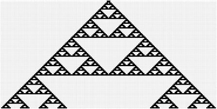
Figure 1. Projection of Equation (4) (with p = q = 1, i.e., rule 126) from a single starting point, forming a structure similar to Sirpinsky's gasket. Horizontal axis is space and vertical axis is time (from early on top to late on the bottom).

$\begin{array}{ll}f(c)=\frac{2}{3}{e}^{\left(\text{ln}(3)\right)(a-n_c)}& (5)\end{array}$

where n_c enumerates the order of the appearance of each cluster size (n₁ for cluster size 2, n₂ for cluster size 4, n₃ for cluster size 6, etc…). Solving Equation (5) for individual cluster sizes (i.e., setting n_c = 1 to solve for the frequency of cluster size two, n_c = 2 for cluster size 4, and so forth) the resulting distribution is given as a near perfect fit to the equation,

$\begin{array}{l}\text{ln}[{\text{f}}_{(\text{c})}]=10.581-1.585\text{ln}(\text{c})\end{array}$

for a = 9. Other values of “a” give the same power function parameter (−1.585) but different intercept values due to larger or smaller numbers of occupied cells. In all cases, the power function fit is almost perfect, leading to the conclusion that the basic model (Equation 4, or equivalently Wolfram's rule 126), generates a power function distribution of cluster sizes, recalling other literature on spatial pattern formation (Pascual and Guichard, 2005; Kéfi et al., 2007; Rietkerk and van de Koppel, 2008; Vandermeer et al., 2008). Adding complications to the model our focus is thus on what sort of deviations from the basic power function are observable.

The generated pattern from a single individual occupied cell, while instructive as a potential foundational pattern, does not capture the complexity of the model. As noted by Wolfram, when initiated with more than 1 individual, complicated patterns emerge in the space/time graph, and they do not seem to undergo any repeated obvious spatial patterns. Nevertheless, perhaps reflecting the underlying tendency to form clusters that are scaled as a power function (as described above for the pattern generated from a single individual), long term simulations seem to generate cluster distributions that are power function scaled, although the distinction between a power function and an exponential function is not clear, as illustrated for a typical example in Figure 2.

FIGURE 2

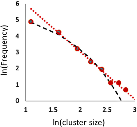
Figure 2. Cluster size distribution for spatial patterns for the last iteration of the standard rule 126 model with no stochasticity and random (μ = 0.5) allocation of starting positions on a one-dimensional lattice of size 2000, after 200 time steps. Dashed (black) curve is an exponential fit to the lower six points (R² = 0.99) and dotted (red) line a power function fit to the higher seven points (R² = 0.99). Bin sizes = 1–3; 3–5; 5–7….

Exploring the stochastic version of the model (i.e., with p and q as random variables), several clear cluster pattern forming scenarios are recognizable, four examples of which are illustrated in Figure 3. An initial observation is that the model produces not only clusters, but frequently distinct clusters of clusters. As a time series is initiated, a not unexpected group of clusters emerge from the initial instantiation, a single cluster from each occupied cell. For example, in Figure 3A ~16 clusters emerge rapidly from the initial condition (where a random 50% of sites were initiated). But quickly, after about 15 time steps, a clear pattern of three groups of clusters, referred to hereafter as megaclusters, are formed. Each megacluster has smaller clusters situated within it, but viewed over the whole landscape (a one-dimensional landscape of time length 300—Figure 3A) three megaclusters are clearly visible (one at about 30, one at about 55 and one at about 65).

FIGURE 3

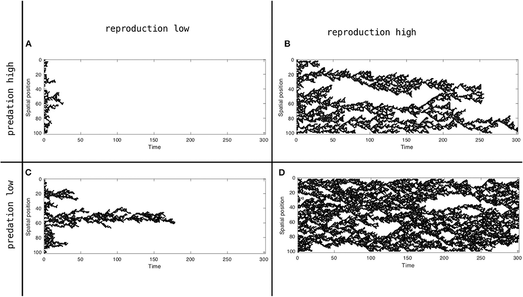
Figure 3. Spatial position (y axis) over time (x axis) realization of the model represented by system 4, for two migration (p) and two predation (q) probabilities (p = 0, 0.5, q = 0, 0.5). (A) With reproduction low and predation high. (B) With reproduction high and predation high. (C) With reproduction low and predation high. (D) With reproduction high and predation low.

It is not a surprise that the model's ability to continue predicting a space filled with the population, as well as its failure to do so, is a function of the migration and predation coefficients. The population in Figure 3A goes extinct after 25 time steps, not surprising since it is the population with low reproduction (migration) facing high predation. The population in Figure 3B forms several distinct megaclusters. For example, at ~80 time steps there are three distinct clusters of clusters, but at about 110 time steps the lower two clusters of clusters seem to merge and only two clusters of clusters seem to exist for a period of time. Then, at about time 200 the remnants of the lower cluster of clusters merges with the upper one and by time 250 that combined cluster of clusters disappears. This structure of metaclusters can be seen in the distribution of the keystone ant species Azteca sericeaseur on a large organic coffee farm in Mexico (Vandermeer et al., 2008, 2019; Li et al., 2016). The species nests in shade trees and regularly abandons particular shade trees, moving on to nearby shade trees, thus forming clusters. But when local nest density becomes too high, a parasitic fly in the family phoridae attacks the nests, to which they respond by moving the nests. The basic arrangement has been likened to the fundamental Turing mechanism (Vandermeer et al., 2008, 2019; Jackson et al., 2014b) and can be likened to Equation (4), which is to say, Wolfram's rule 126. The expectation of a megacluster pattern can be approximately seen from a map of the nests of this ant species, as displayed in Figure 4.

FIGURE 4

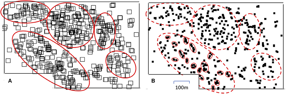
Figure 4. The distribution of nests of the tree-nesting ant species Azteca sericeasur on an organic coffee farm in Chiapas Mexico, in year 2016. (A) Position of nests represented by large squares to suggest the large scale clusters existing in the system, a qualitative correspondence with the expectation from rule 126 (red ovals indicate approximate extent of the proposed five megaclusters). (B) Same positions of nests represented by small black squares revealing the substructure of each of the five megaclusters identified in a, with small ovals identifying the subclusters in the lower left megacluster.

The 1D approximation to population growth in space according to rule 126 reveals something of a deep structure that may be indicative of the behavior of the related 2D models. In particular there is a critical point at which the population crashes (Figure 5), as is the case in the 2D equivalent model (Vandermeer and Jackson, 2015), and as has been reported for similar spatial models (e.g., Rietkerk and van de Koppel, 2008). This evident criticality has been suggested as a model of population extinction as a critical transition (Kéfi et al., 2011), here replicating more complicated models with the excessively simplistic model based on rule 126 (equation set 4). Suggesting there is a critical transition with a model as simple as rule 126 might imply that other more complicated models, and situations in the real world, experience such a transition for a deep reason, rule 126. Much as the Ising model predicts a critical transition for ferromagnetism responding to temperature, we have a very simple model that makes this evident qualitative prediction.

FIGURE 5

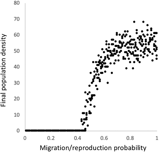
Figure 5. The relationship between the migration coefficient and the final population density (based on a time series of 200 on a space of 100 with random initiation at a probability of 0.5) for the model represented by equation set 4, essentially a stochastic equivalent to Wolfram's rule 126.

Thus, this extremely simplified model of spatial dynamics, constructed as an imitation of a Turing process, does indeed produce certain patterns that correspond to previously observed ones, both in more complicated models (Vandermeer et al., 2008; Jackson et al., 2014b) and empirical data (Figure 4). Power function (or exponential) patterns are produced associated with cluster sizes (Figure 2) and the extinction of the system emerges at a critical state (Figure 5).

The Structure of Chaos in Peasant Agriculture: Simon's Bounded Rationality

There is a multitude of issues that emerge in agroecosystems when thinking of them broadly and realistically, that is, in terms of the actual way in which food and other agricultural products are produced, not in terms of trying to optimize yields or other arbitrary variables (Vandermeer et al., 2018; Perfecto et al., 2019a,b). One of those issues is the interplay of ecology and economics, an issue whose importance is evident by the existence of a journal, Ecological Economics, that seeks to publish academic work on the subject. In terms of small-scale agriculture embedded in some sort of market structure, I envision a set of constraints and opportunities faced by this farming sector that set the stage for a general and realistic understanding (Levins, 1966) of the system as a combined economic and ecological system.

Peasant farmers regularly face many constraints and opportunities. Balancing all of them is a complex process, causing some analysts to situate the peasant economy outside of standard economic assumptions of utility maximization (Ploeg, 2012). Recently a more quantitative approach (Rosser, 2006; Holt et al., 2011) has treated effectively the same problem, challenging the rational economic assumptions of neoclassical economics with the more nuanced notion of “bounded rationality” as elaborated originally by Herbert Simon (Simon, 1957; Rosser, 2006). It seems that the classical approach of Chayanov (Ploeg, 2013), while extremely qualitative, overlaps considerably with the fundamentally quantitative framing of Simon and later “complexity economists,” especially as it applies to small-scale, or peasant, agriculture.

An additional constraint placed on all farming is the “ecological blowback” that sometimes emerges surprisingly, sometimes predictably but nevertheless ignored, and sometimes anticipated and acknowledged in planning. Actual data on this issue is abundant, but not necessarily without controversial interpretation. For example, large-scale monocultures have been implicated in the evolution of resistant varieties of pest species, which then have an impact on future production. Or extensive use of NPK fertilizers in a large river basin can generate hypoxic coastal waters upon runoff. For purposes of this article I presume that there are potentially negative environmental/ecological consequences that emerge from different production regimes, and that there is some sort of critical point at which that blowback is likely to come into effect.

Among the variety of decisions small-scale and peasant farmers must face each year is what mixture of crops they should plant each planting season, acknowledging that conditions at planting time are likely to be different than conditions at harvest. For those crops destined for unconstrained markets, and for which “profits” are sought (i.e., not family consumption or gift-giving or comparable activities), expectations of market price at harvest time is partially predicted by market price at planting time, but with clear constraints. For example, in interviews with small-scale vegetable producers in Costa Rica (Vandermeer, 1990), it was discovered that current market price predicted the proportion of the farm to be planted in tomatoes, but with a curious constraint. At very low market prices any increase in price yielded the expected plan to increase planting of tomatoes. Yet a point was reached at which expected planting proportion declined rapidly with increased current market price. When queried about the origin of this unexpected result, all the interviewees had the same response—when market prices get too high, everyone will plant tomatoes and the market will crash. Effectively their decision-making would result in no one planting tomatoes because everyone is planting tomatoes, recalling the famous Yogi Berraism that “no one goes there anymore, it's too crowded” (O'Toole, 2014). The farmers are effectively creating a situation where no one plants tomatoes because everyone plants tomatoes, a decision bounded by their social expectations.

Formally the situation is known in the analytical literature as the El Farol Bar problem (Huberman and Hogg, 1988) and has seen a variety of formulations (Gintis, 2009), representing a metaphor for many actual real-world applications. Here I present the problem as strictly one of agricultural production in an ecological and economic situation on the border of pure peasant production (use-value realized within the farming family) and market adjustment (selling in unpredictable markets), something on the way to the “entrepreneurial farmer” (Ploeg, 2012). Biological reality imposes a necessary time lag between planting decision and market realization, such that P(t+1) (price at time t+1) is a function of P(t), where unit time is one agricultural season. Taking the data from previous work (Vandermeer, 1990), we apply the equation:

$\begin{array}{ll}H(t)=aP(t)e^{-bP(t)}& (6)\end{array}$

where H is hectares planted, P is price, the parameter a represents the increase in planting intention at low prices and b is an estimate of the risk anticipated from market failure. Note that in this initial formulation H refers to the proportion of a particular farm planted with the crop (H = % of farm size), yet below we generalize H to refer to the total area planted in a region. Formally we could make the transition by multiplying the first meaning by total cumulative farm area in the region, but the generalizations developed here would not change so we leave this small ambiguity in the variable's meaning, for ease of presentation. Equation (6) is applied to the data in Figure 6.

FIGURE 6

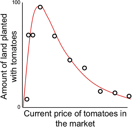
Figure 6. Farmer's planting participation [H(t) = expected percentage of land devoted to tomato production] as a function of the current (planting time) price of tomatoes on the market (data reported in Vandermeer, 1990).

As a first approximation we presume that the actual market price at harvest time is a linear function of the hectares planted, P(t+1) = K - cH(t) (clearly an approximation, but convenient for analytical purposes—see below), and compose the two functions to obtain:

$\begin{array}{ll}P(t+1)=K-AP(t)e^{-bP(t)}& (7)\end{array}$

where A = ac. Differentiating,

$\begin{array}{ll}\frac{dP(t+1)}{dP(t)}=A{e}^{-bP(t)}\left[bP(t)-1\right]& (8)\end{array}$

whence we see a saddle node bifurcation at,

$\begin{array}{l}\frac{1}{bP(t)-1}=a{e}^{-bP(t)}\end{array}$

suggesting two roots and thus two bifurcation points leading to alternative equilibria, as illustrated in Figure 7.

FIGURE 7

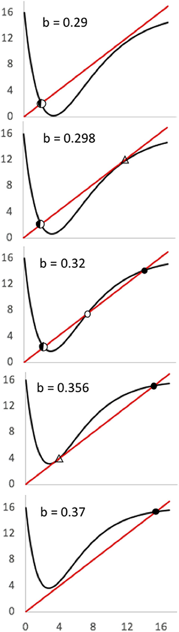
Figure 7. Sequence of bifurcation of Equation (7) (K = 16, a = 4.579).

Differentiating a second time, so as to determine where the inflection points are, we find,

$\begin{array}{l}\frac{d{P}^2(t+1)}{d{P(t)}^2}=A{e}^{-bP(t)}\left[2-b{P(t)}^2\right]\end{array}$

Hence, when there exist three equilibria, the middle one (the unstable one—see Figure 5) will be at the point where the second derivative switches from positive to negative, thus giving,

$\begin{array}{l}{P}_2^{*}(t)=\frac{\sqrt{2}}{b}\end{array}$

whence we see that if the slope of the function at P(t) = $\frac{\sqrt{2}}{b}$ is 1.0, one of the two bifurcation points will exist there. It is thus evident that bifurcating on the parameter b will generate the two bifurcations illustrated in Figure 5A and ultimately a hysteritic pattern is generated, in which the two bifurcation points define the critical transitions. An exemplary bifurcation sequence is presented in Figure 8.

FIGURE 8

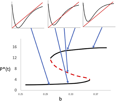
Figure 8. Critical transition and hysteresis emerging from the dual saddle/node bifurcations.

Further complications emerge with other parameter combinations. For example, various patterns of chaos may emerge when,

$\begin{array}{l}1<A{e}^{{-bP}_1^{*}}\left[b{P}_1^{*}-1\right]\end{array}$

where $P_1^{*}$ refers to the lower stable equilibrium point (that originally emerged from the first saddle/node bifurcation) as illustrated in Figure 9. The emergence of chaos is well-known in this sort of model (discrete maps) to occur when the derivative of the function evaluated at its intersection with the one-to-one line is <-1, generating the typical sensitive dependence on initial conditions. The rest of the function may be increasing or decreasing exponentially, the important point being that the trajectory is exponentially diverging from the equilibrium. In particular at,

$\begin{array}{l}\frac{\sqrt{2}}{b}=K-\frac{A^2}{eb}{e}^{-\frac{A}{e}}\end{array}$

a basin boundary collision occurs (Vandermeer and Yodzis, 1999), effectively separating a range of a single chaotic attractor from alternative attractors, one of which is chaotic (Figure 9).

FIGURE 9

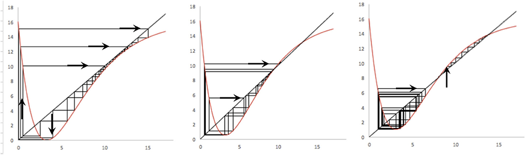
Figure 9. Chaotic patterns in the basic model (K = 16; A = 4.8). (Left) Simple chaotic attractor centered on the lower equilibrium point (b = 0.3). (Middle) Basin/boundary collision where the lower chaotic “attractor” eventually gives way to the upper equilibrium point (b = 0.31). (Right) Alternative equilibria, in which the lower point is a chaotic attractor (b = 0.32) and the upper point a node.

While the basic equation and the system it is thought to represent yields a rich dynamical diversity (dual saddle/node bifurcations, critical transitions and hysteresis, chaos, basin boundary collision), the formation is less useful for interpreting the qualitative nature of the real-world system it seeks to represent. A more useful approach, that retains all of the dynamic diversity of Equation (7), is a simple tent-map formulation, composing the two relevant functions, with the price to production function a simple tent map and the production to price function a simple linear function (as in the composition that produced Equation (7). The various points of discontinuity then are easy to interpret. The relevant map, referred to as a tent map even though it is sort of an upside-down tent map with an extended tail, is illustrated in Figure 10. It is evidently a linear approximation to Equation (2).

FIGURE 10

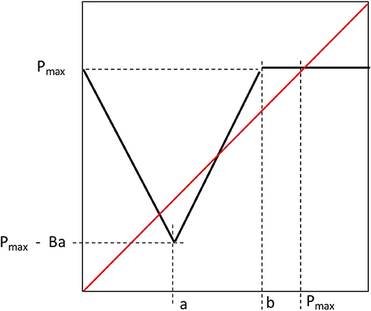
Figure 10. Linear approximation to Equation (7), an inverse tent map with a tail.

The composition producing this tent map was of three linear functions for P(t) < a. The slopes of those functions are α, γ, and -δ, respectively, for the map of P(t) to H(t), H(t) to Y(t), and Y(t) to P(t+1) respectively. When 0 < a P(t) < b the map of P(t) to H(t) has negative slope of -β, with the intercept on the x axis = b. The equations for this piece-wise linear map are (with composite parameter B = αγδ):

$\begin{array}{ll}{P}_{t+1}=P_{max}-B{P}_{t}for0<P_t<a& (\mathrm{9a})\end{array}$

$\begin{array}{ll}{P}_{t+1}=P_{max}-\frac{Bab}{b-a}+\frac{Ba}{b-a}{P}_{t}fora<P_t<b& (\mathrm{9b})\end{array}$

$\begin{array}{ll}{P}_{t+1}=P_{max}forb<P_t& (\mathrm{9c})\end{array}$

where the three boundary parameters all have obvious real-world meanings: P_max is the highest price that a unit of production could ever command, a is the price that separates the increasing production decisions from the risk aversion mode, the “critical risk price,” and b is the price of “economic collapse” where the price is so high that all farmers decide to not engage in the relevant activity (all decide that the market will collapse). The bifurcation points are then evident from a glance at the graph (Figure 10), wherein the first saddle/node bifurcation occurs when b = P_max, which is to say when the economic collapse price is equivalent to the maximum price, and the second saddle/node bifurcation occurs when P_max = a(1-B). The actual value of P_max is of obvious importance for both bifurcation points, but it can also be said that the first bifurcation point is conditioned by the economic collapse parameter (b) while the second is conditioned by the critical risk price (a). The slope of the descending limb of the function will determine the nature of the lower equilibrium, and thus the potential for chaotic oscillations. That slope is the parameter B [equal to the linear compositions for P(t) < a, which is to say αγδ]. If B < 1, the second “node” that came from the second bifurcation, will in actuality be a chaotic attractor, which will be true if there is a fixed point at that location, which is to say, if a(1 + B) < P_max. Finally, a basin-boundary collision will occur if (1) the lower fixed point is chaotic and the projection from P(t) = a, is above the unstable fixed point,

Adding the Negative Consequences of the Industrial Mode of Production

A key element enters into reflections about the state of agriculture in its industrial form. Some analysts argue that as a particular monocultural form of production (or even the simple extension of production) increases, the potential for ecological damage that eventually feeds back negatively on that same production, increases. In other words, in terms of the amount of production (Y = yield), it is not adequate to simply translate P(t+1) = K - cH(t), since at very high levels of H, actual production is expected to decrease and thus P(t+1) increases accordingly. Thus, the model requires an ecological constraint on production. In the absence of generalizable knowledge (other than the expected increase in Y as H increases at low levels but an expected decrease in Y as H increases at high levels) I propose a simple quadratic approach, namely, Y(t) = gH(t) - hH(t)². Whence the general price trajectory (change in price over time) is given as (retaining the linear relationship between Y and P),

P(t+1) = P_max – kY(t),

substituting for Y,

P(t+1) = P_max – k[ gH(t) - hH(t)²],

and substituting for H (from Equation 6),

$\begin{array}{ll}P(t+1)=P_{\text{max}}-P(t)e^{-bP(t)}\left[B-CP(t)e^{-bP(t)}\right]& (9)\end{array}$

where B = kga and C = kha². It is evident that at P → 0 or P → ∞, P(t+1) = P_max, as is also the case in Equation (2). Differentiating,

$\begin{array}{l}\frac{dP(t+1)}{dP(t)}=e^{-2b{P}_t}\left[\left(b{P}_t-1\right)\left(B{e}^{b{P}_t}-2C{P}_t\right)\right]\end{array}$

whence we see four roots, counting P → ∞, and, by graphical inspection four separate saddle/node bifurcations, as illustrated in Figure 11.

FIGURE 11

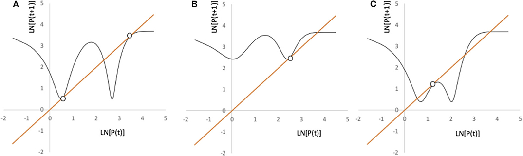
Figure 11. Illustration of the four possible bifurcation points for the model in Equation (3). Parameters for all three panels are P_max = 40, g = 1.1, and k = 5.4. (A) b= 0.17, a = 10.5, h = 0.0426. (B) b = 0.24, a = 12, h = 0.057. (C) b = 0.24, a = 10.5, h = 0.0424.

A simple examination of the bifurcation points (Figure 11) provides a generalized picture of the possible dynamic behavior of this model, which is complex, including chaotic trajectories, chaotic transients, catastrophic transitions, and alternative chaotic attractors. However, a more intuitive and qualitative analysis is possible if we take the piece-wise linear approach, as above, wherein critical points with ecological and economic significance are evident. This analysis is illustrated in Figure 12.

FIGURE 12

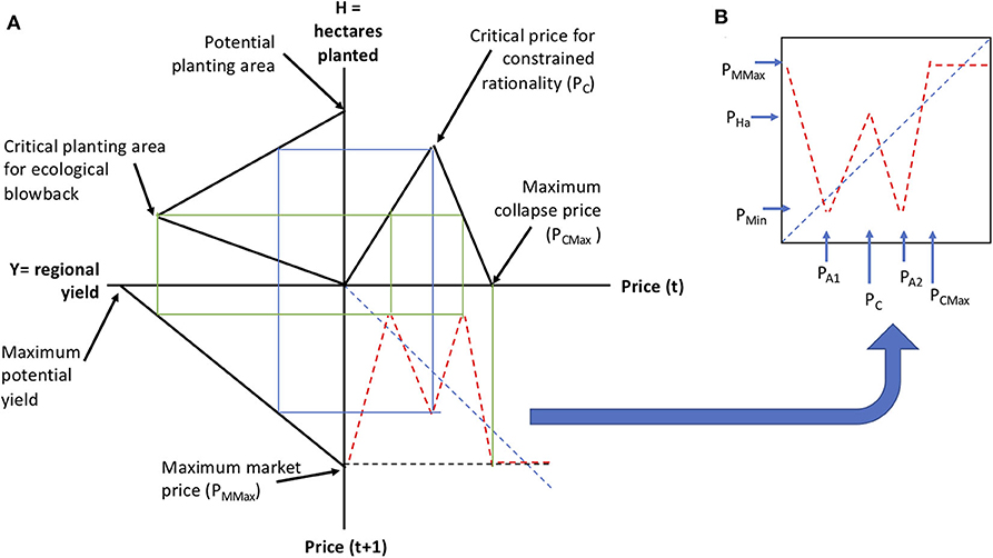
Figure 12. Composed form of the piece-wise linear function approximation to Equation (3). (A) Illustration of the composition process. (B) The resulting composed function.

In this formulation (Figure 12) there are six readily interpreted parameters (1) Maximum collapse price, which is the observed price that causes the farmer to decline planting any of the crop in question, (2) the critical price for constrained rationality, which is that price for which there is a switch from responding positively to the key market signal to one of restraint in anticipation of possible market collapse, (3) the potential planting area, which is the maximum amount of hectares that could be planted in this crop, (4) critical planting area for ecological blowback, which is the point where ecological damage begins to overtake potential yield from more planting, (5) Maximum potential yield, which is the ecologically limited maximum per hectare yield of the crop, (6) the maximum market price, which could be larger than the maximum collapse price.

The qualitatively distinct forms that emerge from the manipulation of the parameters of this model are varied, as illustrated in Figure 13. Note that there is a potential for six distinct equilibrium points (Figure 13A), of three general types. First, symbolized with a closed circle in Figure 13 is a stable equilibrium point, second, symbolized with an open circle is an unstable point and third, symbolized with a half circle are points that may be either stable points or loci of a chaotic attractor, depending on the eigenvalue (slope of the function where it crosses the 45 degree line).

FIGURE 13

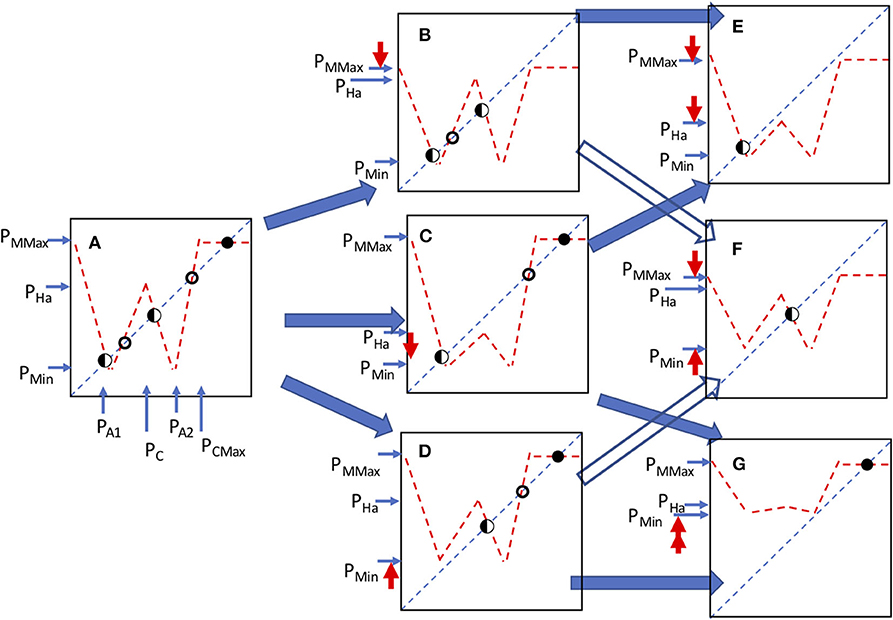
Figure 13. All the qualitatively distinct structural arrangements of the model. Circles indicate the position and nature of the equilibrium points, an open circle indicates an unstable point, closed circle a stable point and half closed circle is either a stable point or the focus of a chaotic attractor, depending on the eigenvalue. Bold (red) arrows pointing up or down indicate the parameter change in going from one panel to the next, according to the dark (blue) shaded arrows indicating change from panel to panel. A is original orientation. A moves to either B, C, or D, depending on the parameter change indicated by the red arrows going up or down. B moves to either E or F depending on parameter change indicated by the red arrows, C moves to either E or G depending on parameter change indicated by the red arrows, D moves to F or G depending on parameter change indicated by the red arrows.

From the point of view of stable points, there is a rather limited set of behaviors that can emerge, as illustrated in Figure 13. These various critical points can be interrogated individually to explore the potential dynamics of the resulting composed function. For example, in Figure 14 illustrate the changes in the critical planting density that give rise to ecological blowback and how it can change the dynamics from a stable point to a chaotic trajectory constrained within a small range of state space to a qualitatively similar dynamic behavior but within a dramatically enlarged range of state space.

FIGURE 14

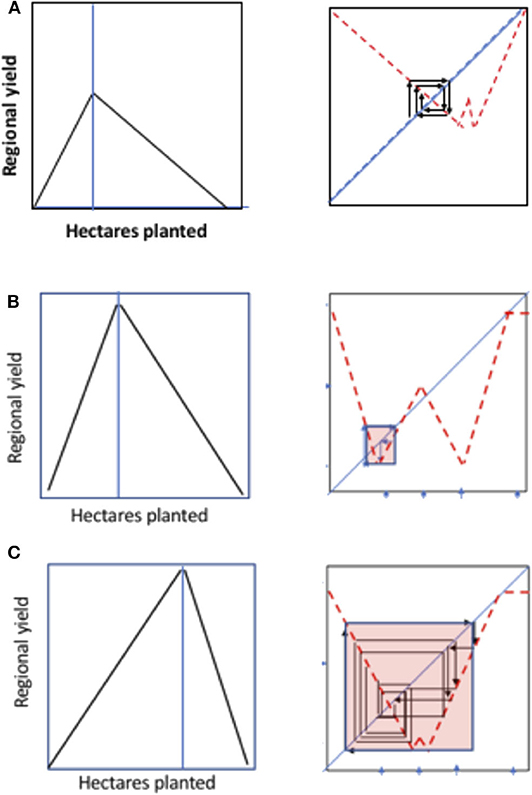
Figure 14. Illustration of changed dynamics resulting from an increase in the critical planting density that gives rise to ecological blowback. (A) Reduced expected yield at critical planting density (i.e., density at which ecological decline begins) and reduced planting density, yielding a stable equilibrium point. (B) High expected yield and reduced critical planting density yielding a “constrained” chaotic attractor. (C) High expected yield and increased critical planting density yielding an “expansive” chaotic attractor.

As is evident in Figure 14, interrogation of individual biologically meaningful parameters graphically can easily generate the expected changes in the overall system (i.e., the resulting 1D map relating price at planting time with price at harvest time). Alternative states are clearly possible, indeed common, and under proper hypotheses of how parameters change, hysteretic patterns arise under many different parameter combinations. An interesting qualitative generalization seems to also emerge—although behavior of the system is dependent in a complicated way on the interaction of all parameters in the model, there seems to be a qualitative generalization about the nature of emerging chaotic attractors, as shown graphically in Figure 13. The critical parameters, so easily identified in the linear approximation model (equation set 9) can thus be easily visualized as changing the overall dynamics of the system in qualitatively distinct ways. Figure 14 is one such example.

Discussion

The now moribund tendency toward positivism in the social sciences was a result of a desire to emulate the evident successes of the physical sciences, creating a true “science” out of the collection of intellectual currents that constituted the study of Homo sapiens. It was thought that perhaps the optimism (or arrogance) that the Newtonian Revolution engendered could be penetrated by the lessons that social scientists have come to learn. In particular the so-called nomothetic tendencies of disciplines such as sociology or economics, which seek universal mechanisms that explain the foundations of human social behavior, can be contrasted with the more idiographic tendencies of disciplines such as anthropology or history (the latter frequently, and inexplicably, categorized as a subject of the humanities), which seek detailed understanding of particulars. This is a fundamental insight of Wallerstein (2004) (writing of Braudel and the Annales school of French social science in 2004). Precisely the same insight is repeated in modern complexity science and its approach to social science, what might be initially demeaned, unfairly in my view, as positivism. As Miller and Page (2009) note, most social science theorizing is carried out at one or the other end of a continuum, either at the level of a small number of individuals (e.g., much social psychology) or at the level of an infinite population (much of microeconomics). In contrast to this theorizing, most real world social dynamics in fact occur somewhere in between. Our focus should not be either the idiographic (small groups localized in time and space), nor the nomothetic (extremely large populations, with universal rules thus negating the need for time and/or space stipulations). Since reality lies in between, our theorizing should likewise be focused there.

Ecology generally, and most importantly agroecology, faces a similar dilemma. The very “old-fashioned” approach in the style of eighteenth century naturalists remains the preferred approach of both modern naturalists and experimentalists, from the tangled bank of Darwin to the Biophilia of E. O. Wilson. Accompanying this narrow focus is the application of specific quantitative models to specific situations, mainly using Lotka-Volterra-style approaches to small groups of species or functional groups, similar in philosophy to the idiographic approaches of some social scientists (e.g., most anthropologists). Yet MacArthur and Wilson's island biogeography or Levins' metapopulations present a completely different perspective, focusing on a mean field philosophy that resembles the nomothetic thrust of other social scientists (e.g., economists). Is there, in ecology, a middle ground, a set of conceptualizations that free us from the gravitation toward either of these two poles?

Recall that Newton's mechanical universe became popular during the exuberance of the young Industrial Revolution, where mechanical devices marshaled the magic of levers and gears in very complicated ways to create all sorts of complicated devices. Newton's mathematization of motion enabled precise control and thus manufacturing manipulation of everything from locks to clocks. As Jacob (1976, 1997) notes in her history of the Newtonian frenzy, the new science became the cause celebré of the day, with popular demonstrations drawing huge crowds of spectators. The complicated devices that transformed energy from its potential to its use, whether from the pulsations of the pistons of a steam engine or the oscillating pendulum of a clock, made it seem that the entire world was constructed of such mechanical devices. Yet, it is worth recalling that the reception of Newtonism on the continent was rather distinct from in England. The latter seems inextricably tied up with the Industrial Revolution while the continental reception was more as a philosophical issue, as a new understanding of the way the world works, rather than the English focus on instrumentalism (Jacob and Stewart, 2004).

The science of ecology has evolved in what might be construed as a similar fashion. On the one hand, wildlife managers and biological control technicians combined field observations, controlled laboratory studies, and mathematical models to construct models of their systems that rivaled the most complicated work of civil engineers. On the other hand, population geneticists worked with populations containing infinite numbers of individuals and community ecologists studied communities with very large numbers of identical species. The science of ecology thus has its ideographic vs. nomothetic contextualization also. Might the intent to utilize concepts from complex systems in ecology be ultimately more acceptable in a more applied aspect of ecology, agroecology.

Regardless, it is arguably the case that even the simplest assumptions, relevant to actual operation of the agroecosystem, can give rise to unexpected, but interesting and potentially important consequences. The basic Turing process is almost certain to operate at a landscape level for many pest control situations, generating a patchiness that, on the one hand, could befuddle attempts at generating control strategies, but, on the other hand, if properly understood could provide for large scale management of the control system. For example, the green coffee scale insect (Coccus viridis) has an important association with the aggressive tree-nesting ant Azteca sericeasur (Vandermeer and Perfecto, 2006). It is attacked by both a predator (a coccinellid beetle, Azya orbigera) and a fungal pathogen (Lecanicillium lecani). Receiving protection from the beetle predator from the mutualistic relationship with the ant, it builds up very large populations, but locally within the clusters of the ant nests. Its complicated relationship with its two control agents (Vandermeer and Perfecto, 2019) is conditioned on the clustered distribution of the ant nests. Those clusters are formed by the action of a parasitic fly (Pseudacteon spp.) acting in familiar Turing fashion (Alonso et al., 2002), creating power law scaling for the ant clusters (Vandermeer et al., 2008). Understanding this complicated relationship, involving not only Turing dynamics but also such complex systems topics as hysteresis, critical transitions, and basin/boundary collisions (Vandermeer and Perfecto, 2019), enables clear practical recommendations (e.g., eliminate the shade trees and expect the scale insect to increase in importance as a pest).

The real world of the agroecosystem, as repeatedly emphasized by those in the agroecological movement, involves all the sociopolitical issues surrounding agriculture the world over. Seriously incorporating such issues in the analysis makes the framework of complex systems even more relevant. The example of tomato farmers who anticipate market collapse, at once suggests that the farmers themselves are thoughtful interlocutors in dynamics that extend well-beyond their own interests yet certainly do not anticipate the chaotic complications that will arise from the regional collection of independent farmers with only limited knowledge of what the market will do. The simple model presented herein suggests that, for example, information about general planting patterns will result in a rational collective action to not exceed the critical planting densities and thus not face erratic chaotic swings in production and price trajectories. The case of cellphones in a south Indian fishery is a remarkable example of precisely this phenomenon—what appears to have been a chaotic market in the local fishery, stabilized considerably after the introduction of cell phones (and the concomitant knowledge of what fishing activities in a large region were) (Jensen, 2007).

In this article I have focused on what I propose are the two central issues of complexity science as it might form a foundation for agroecosystem ecology, perhaps even ecology more generally. Turing instabilities and chaos form a couplet that seems to be a sort of foundation for other topics that commonly are associated with the study of complex systems. The issue of coupled oscillators, for instance, becomes an especially interesting topic in the light of chaotic oscillations. Critical transitions are well-known to be associated with spatial patterns, many of which can be thought of through the lens of Turing instabilities. These and other topics that have become standard fare in the emerging field of complex systems, are applied in many disciplines, providing new insights. The application in ecology is also active, but the application specifically to agriculture, especially the sort of agriculture commonly known as agroecology, is only beginning (Vandermeer and Perfecto, 2017).

Data Availability Statement

The raw data supporting the conclusions of this article will be made available by the authors, without undue reservation, to any qualified researcher.

Author Contributions

JV wrote the article.

Funding

This work was supported by National Science Foundation DEB-1853261.

Conflict of Interest

The author declares that the research was conducted in the absence of any commercial or financial relationships that could be construed as a potential conflict of interest.

References

Alonso, D., Bartumeus, F., and Catalan, J. (2002). Mutual interference between predators can give rise to turing spatial patterns. Ecology 83, 28–34. doi: 10.1890/0012-9658(2002)083[0028:MIBPCG]2.0.CO;2

CrossRef Full Text | Google Scholar

Gintis, H. (2009). Game Theory Evolving. Princeton, NJ: Princeton University Press.

PubMed Abstract | Google Scholar

Haeckel, E. (1870). Generelle Morphologie der Oganismen: Allgemeine Grundzuge der Organischen Formenwissenschaft. Mechanisch Begrundt Durch die von Charles Darwin Reformirte Descendenz-Theorie. Berlin Vorlag von George Reiner.

Google Scholar

Holt, R. P. F., Rosser, J. B., and Colander, D. (2011). The complexity era in economics. Rev. Political Econ. 23, 357–369. doi: 10.1080/09538259.2011.583820

CrossRef Full Text | Google Scholar

Huberman, B. A., and Hogg, T. (1988). “The Ecology of Computation: Studies in Computer Science and Artificial Intelligence,” in Digest of Papers. COMPCON Spring 89. Thirty-Fourth IEEE Computer Society International Conference: Intellectual Leverage (Los Angeles, CA: IEEE), p. 362.

Google Scholar

Jackson, D., Vandermeer, J., Allen, D., and Perfecto, I. (2014a). Self-organization of background habitat determines the nature of population spatial structure. Oikos 123, 751–761. doi: 10.1111/j.1600-0706.2013.00827.x

CrossRef Full Text | Google Scholar

Jackson, D., Vandermeer, J., Perfecto, I., and Philpott, S. M. (2014b). Population responses to environmental change in a tropical ant: the interaction of spatial and temporal dynamics. PLoS ONE 9:97809. doi: 10.1371/journal.pone.0097809

PubMed Abstract | CrossRef Full Text | Google Scholar

Jacob, M. C. (1976). The Newtonians and the English Revolution, 1689-1720. Ithaca, NY: Cornell University Press.

Google Scholar

Jacob, M. C. (1997). Scientific Culture and the Making of the Industrial West. Oxford.

Google Scholar

Jacob, M. C., and Stewart, L. (2004). Practical Matter: Newtons Science in the Service of Industry and Empire, 1687-1851. Cambridge: Harvard University Press.

Google Scholar

Jensen, R. (2007). The digital provide: information (technology), market performance, and welfare in the South Indian fisheries sector. Q. J. Econ. 122, 879–924. doi: 10.1162/qjec.122.3.879

CrossRef Full Text | Google Scholar

Kéfi, S., Rietkerk, M., Alados, C. L., Pueyo, Y., Papanastasis, V. P., ElAich, A., et al. (2007). Spatial vegetation patterns and imminent desertification in Mediterranean arid ecosystems. Nature 449, 213–217. doi: 10.1038/nature06111

PubMed Abstract | CrossRef Full Text | Google Scholar

Kéfi, S., Rietkerk, M., Roy, M., Franc, A., de Ruiter, P. C., and Pascual, M. (2011). Robust scaling in ecosystems and the meltdown of patch size distributions before extinction. Ecol. Lett. 14, 29–35. doi: 10.1111/j.1461-0248.2010.01553.x

PubMed Abstract | CrossRef Full Text | Google Scholar

Levins, R. (1966). The strategy of model building in population biology. Am. Sci. 54, 421–431.

Google Scholar

Li, K., Vandermeer, J., and Perfecto, I. (2016). Disentangling endogenous versus exogenous pattern formation in spatial ecology: a case study of the ant Azteca sericeasur in southern Mexico. R. Soc. Open Sci. 3:160073. doi: 10.1098/rsos.160073

PubMed Abstract | CrossRef Full Text | Google Scholar

Miller, J. H., and Page, S. E. (2009). Complex Adaptive Systems: An Introduction to Computational Models of Social Life, Vol. 17. Princeton, NJ: Princeton University Press.

Google Scholar

Morales, H., and Perfecto, I. (2000). Traditional knowledge and pest management in the Guatemalan highlands. Agric. Hum. Values 17, 49–63. doi: 10.1023/A:1007680726231

CrossRef Full Text | Google Scholar

O'Toole, G. (2014). Quote Investigator. Available online at: https://quoteinvestigator.com/2014/08/29/too-crowded/ (accessed June 16, 2020).

PubMed Abstract | Google Scholar

Pascoe, B. (2018). Dark Emu: Aboriginal Australia and the Birth of Agriculture. London: Magabala Books.

Google Scholar

Pascual, M., and Guichard, F. (2005). Criticality and disturbance in spatial ecological systems. Trends Ecol. Evol. 20, 88–95. doi: 10.1016/j.tree.2004.11.012

PubMed Abstract | CrossRef Full Text | Google Scholar

Perfecto, I., Jiménez-Soto, M. E., and Vandermeer, J. (2019a). Coffee landscapes shaping the anthropocene: forced simplification on a complex agroecologoical landscape. Curr. Anthropol. 60, 5236–5250. doi: 10.1086/703413

CrossRef Full Text | Google Scholar

Perfecto, I., Vandermeer, J., and Wright, A. (2009). Nature's Matrix: Linking Agriculture, Conservation and Food Sovereignty. London: Routledge.

Google Scholar

Perfecto, I., Vandermeer, J., and Wright, A. (2019b). Nature's Matrix: Linking Agriculture, Conservation and Food Sovereignty, 2nd Edn. London: Routledge.

Google Scholar

Ploeg, J. D. V. D. (2012). The New Peasantries: Struggles for Autonomy and Sustainability in an Era of Empire and Globalization. New York, NY: Routledge.

Google Scholar

Ploeg, J. D. V. D. (2013). Peasants and the Art of Farming: a Chayanovian Manifesto. Winnipeg, NS: Fernwood Publishing.

Google Scholar

Potter, L. M. (1996). The dynamics of Imperata: historical overview and current farmer perspectives, with special reference to South Kalimantan, Indonesia. Agroforestry Syst. 36, 31–51. doi: 10.1007/BF00142866

CrossRef Full Text | Google Scholar

Rietkerk, M., and van de Koppel, J. (2008). Regular pattern formation in real ecosystems. Trends Ecol. Evol. 23, 169–175. doi: 10.1016/j.tree.2007.10.013

PubMed Abstract | CrossRef Full Text | Google Scholar

Rival, L. (2005). “The growth of family trees: understanding Huaorani perceptions of the forest,” in: The Land Within: Indigenous Territory and the Perception of Environment, eds A. Surrallés and P. G. Hierro (Copenhagen: IWGIA, 90–109.

Google Scholar

Rosser, J. B. Jr. (2006). “Complex dynamics and post Keynesian economics,” in: Complexity, Endogenous Money and Macroeconomic Theory, Essays in Honour of Basil, ed J. Moore. (Cheltenham: Edward Elgar, 74–98.

Google Scholar

Simon, H. A. (1957). Models of Man; Social and Rational. Hoboken: Wiley.

Google Scholar

Toffoli, T., and Margolus, N. (1987). Cellular Automata Machines: A New Environment for Modeling. Cambridge: MIT Press.

Google Scholar

Vandermeer, J. (1990). Notes on agroecosystem complexity: chaotic price and production trajectories deducible from simple one-dimensional maps. Biol. Agric. Horticulture 6, 293–304. doi: 10.1080/01448765.1990.9754529

CrossRef Full Text | Google Scholar

Vandermeer, J., Aniket, A., Allgeier, J., Badgley, C., Baucom, R., and Blesh, J. (2018). Feeding prometheus: an interdisciplinary approach for solving the global food crisis. Front. Sustain. Food Syst. 2:39. doi: 10.3389/fsufs.2018.00039

CrossRef Full Text | Google Scholar

Vandermeer, J., Armbrecht, I., de la Mora, A., Ennis, K. K., Fitch, G., Gnthier, D. J., et al. (2019). The community ecology of herbivore reulation in an agroecosystem: lessons from complex systems. BioScience 69:974996. doi: 10.1093/biosci/biz127

CrossRef Full Text | Google Scholar

Vandermeer, J., and Jackson, D. (2015). Spatial pattern and power function deviation in a cellular automata model of an ant population. arXiv [Preprint]. arXiv:151208660.

Google Scholar

Vandermeer, J., and Perfecto, I. (2006). A keystone mutualism drives pattern in a power function. Science 311, 1000–1002. doi: 10.1126/science.1121432

CrossRef Full Text | Google Scholar

Vandermeer, J., and Perfecto, I. (2017). Ecological Complexity and Agroecology. New York, NY: Routledge.

Google Scholar

Vandermeer, J., and Perfecto, I. (2019). Hysteresis and critical transitions in a coffee agroecosystem. Proc. Natl. Acad. Sci. U.S.A. 116, 15074–15079. doi: 10.1073/pnas.1902773116

PubMed Abstract | CrossRef Full Text | Google Scholar

Vandermeer, J., Perfecto, I., and Philpott, S. M. (2008). Clusters of ant colonies and robust criticality in a tropical agroecosystem. Nature 451:457. doi: 10.1038/nature06477

PubMed Abstract | CrossRef Full Text | Google Scholar

Vandermeer, J., and Yodzis, P. (1999). Basin boundary collision as a model of discontinuous change in ecosystems. Ecology 80, 1817–1827. doi: 10.1890/0012-9658(1999)080[1817:BBCAAM]2.0.CO;2

CrossRef Full Text | Google Scholar

Wallerstein, I. M. (2004). The Uncertainties of Knowledge. Philadelphia, PA: Temple University Press.

PubMed Abstract

Wolfram, S. (2002). A New Kind of Science. Champaign, IL: Wolfram Media Inc.

Google Scholar