Multi-Scape Interventions to Match Spatial Scales of Demand and Supply of Ecosystem Services

Introduction

Ecosystem functions and services have characteristic or salient scales at which they operate, which are basically defined by the scales at which the organisms associated with the service operate (Liu et al., 2017). Ecosystem services (ES) are supplied by functions and associated organisms in the habitat or land type they occupy, and they are demanded and consumed by humans. Production of ES depends on the amount of suitable land and density and distribution of corresponding organisms in these lands. The degree to which demand is met depends not only on rate of production but also on the movement and distribution of ES beyond the location where they are produced, which requires flow paths and may include sinks (Bagstad et al., 2013).

The full value of ecosystem services can be realized only when supply and demand are connected by suitable distances and processes. Until recently, most ES studies focused on potential production and supply, neglecting the demand side of the system (Sala et al., 2017). Syrbe and Grunewald (2017) define six spatial relationships between supply and demand: “local,” when supply and demand are in the same area; “proximity,” when they are connected by natural transfer from a service producing area to an adjacent service benefitting areas; “process,” when natural processes transfer services across “service connecting areas” that separate producing and benefitting areas; “access,” when beneficiaries travel to the producing area to enjoy the service; “commodity,” when actors who share in the benefit collect and deliver the goods to beneficiary consumers; and “global,” when the services are naturally distributed to the whole planet and cannot be spatially restricted. Because it is categorical, this classification may be easier to use for regulation and planning than the continuity of distances and arrangements that can be addressed by the framework proposed by Bagstad et al. (2013).

Bagstad et al. (2013) provided a comprehensive basis to evaluate the production and use of ecosystem services that pivots on the idea that areas can be classified as sources, sinks, rival-use and non-rival use of services. Different areas are connected by carriers of ES. User areas may receive more or less of the ES depending on the carrier flow routing because it determines a decay of service with distance and the carrier may be depleted by intervening sinks or rival-use areas. For example, the aesthetic and recreational value of green space decline with distance because beneficiaries have to travel to the source location, which is costly.

Open, green space can be a source (or service providing areas) of multiple ES, including the crucial supply of recreation and opportunity for healthy development. In an epidemiological study involving about 1 million people of Denmark, Engemann et al. (2019) found a strong association between availability of green space within ~210 m of the home during childhood and reduced risk of a wide spectrum of psychiatric disorders later in life, even after correcting for level of urbanization, socioeconomic factors, parental history of mental illness and parental age. Risk of mental disorders and availability of green space exhibited a dose-response relationship. Grasslands and rangelands provide green and open spaces with aesthetic and recreation value, in addition to multiple other ecosystem services (Yahdjian et al., 2015), but those services must reach demand in order to become realized. The characteristics of their spatial distribution is critical.

Spatial distribution of ES demand and supply can be controlled by different factors at different scales. Liu et al. (2017) found that ecosystem service distribution (water purification, water supply, soil retention, and crop production) was controlled by human activities at a scale of 12 km and by abiotic factors at a scale of 83 km in the highly developed and densely populated Taihu Lake Basin in China. For example, grasslands and grazing lands are sources of forage and recycle animal excretions. When animals graze directly at pasture in moderate densities, the spatial distribution of supply and demand at the farm scale can be naturally matched by proper management. However, when animals are concentrated in certain regions, spatial distributions of demand and supply at regional scale become disjoint and can cause environmental damage (Syrbe and Grunewald, 2017), both by requiring transportation based on fossil fuels or by contamination of water. Forage produced that is not directly grazed by livestock can be harvested and becomes a commodity whose benefits can be widely distributed through regular market carriers. Animal waste is increasingly becoming a similar commodity used for fertilization and composting. Because of transportation and handling costs, the net value of the services declines gradually with distance to the user. However, the market for animal waste is much less developed than the hay market, so the value of waste recycling services declines more abruptly with distance.

Production of ES in agricultural landscapes likely depends on the extent of interventions. Lindborg et al. (2017) considered the effects of amount and extent of interventions such as planting hedgerows on the level of ES produced. They proposed four types of responses of ES production to amount of intervention expressed as a proportion of the area where ES are considered (Figure 1). The theory suggests that the same interventions have different effects on ecosystem services that differ in mobility, but also that the same ES responds differently depending on intervention scale. For example, when the extent of the landscape is small, even a large proportion of area devoted to intervention may create limited or no ES if the ES is based on the establishment of a population or community that has a minimum area requirement.

FIGURE 1

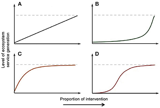
Figure 1. Types of relationships between proportion of area receiving an intervention such as planting of hedgerows or flower strips and level of production of ecosystem services. (A) Linearly increasing ES with intervention proportion. (B) ES that has an ecological threshold to be produced, for example, one that is produced by a species that needs a certain amount of habitat to establish. (C) Rapid saturation of ES production because limiting factors other than intervention. (D) Sigmoid relationship resulting when mechanisms for (B) and (C) take place within the range of proportion of area receiving the intervention. From Lindborg et al. (2017); used under the Creative Commons Attribution License.

The goal of my present work is to further develop the idea that scale affects ES by considering not only extent, but the continuum of spatial distribution characteristics, and by including the interaction with spatial distribution of demand. I consider proportion of ES demand met as a function of type, amount and spatial distribution of intervention with a simple but effective quantitative model and illustrate the effects with examples.

Modeling Framework

I created a static, deterministic model of ecosystem service (ES) supply and demand over space to illustrate the relationship between the proportion of the landscape that receives an intervention and the proportion of ES demand that is met. For simplicity and to prevent errors in the computation of spatial integrals, the model represents space in a single dimension, over a line. Results are quantitatively correct for areas if proportions of lengths are translated into equal proportions of area, instead of squaring them.

First, I describe the components of the model and then I describe simulated examples. Examples use realistic parameter values for three types of ES and organisms that have contrasting characteristics, to explore the impacts of amount and distribution of interventions such as restoration or habitat creation on the quantity of ES demand that is met. The context is a landscape with a patchwork of agriculture, pastures, grasslands, hedgerows and trees where interventions such as habitat creation or reforestation are considered to supply specific ES demanded in the landscape. I selected three examples (carbon sequestration and soil OM provided by oaks, pollination services provided by bumblebees and predation services provided by Northern Harriers) of ecosystem services classified as biotic regulation and maintenance services to show contrasting ratios of minimum intervention size necessary (the “exclusion radius”) and size of the area supplied with ES (kernel radius). The fact that I could provide realistic and understandable simulations with parameters based on published articles also affected my choice of organisms and services.

Ecosystem Service Supply and Demand

Supply

Ecosystem services are provided by functional units (FU) such as individual animals, plants, communities or colonies. Each functional unit requires a certain amount of landscape area treated with an intervention such as a certain type of vegetation that provides nesting habitat and cover in order to exist sustainably. Once a unit occupies its required space, no other FUs of the same kind can occupy it. In the model, the size of the minimum intervention required and preempted by each FU is represented by a radius r_min that is unit specific. Because each FU “uses up” the intervention within r_min, I also refer to it as “exclusion radius,” because no other FU of the same kind can use the same space to establish. Each FU provides one unit of ES that is distributed over space according to a kernel that typically decreases with increasing distance to the center of the intervention. For the cases depicted here, I chose a triweight kernel (Equation 1) as a generic example that can be scaled easily and has finite support. Its single parameter λ is the reciprocal of the radius or extent of the kernel r_k. The kernel has value K(u) when u, the absolute distance to the center of the kernel, is < 1/λ = r_k, and 0 everywhere else. Kernels are specific for the FU and the function or ES under consideration.

$\begin{array}{l}K\left(u\right)=\lambda \frac{35}{32}{\left(1-{\lambda }^2{u}^2\right)}^3\\ support: |u|\le \frac{1}{\lambda }& (1)\end{array}$

The framework that I propose can be used with any kernel desired to study the impacts of amount and distribution of specific functional units on the total amount of services realized. I expect that results will differ depending on the type of kernel used. Although I use realistic examples, the model is for specific illustration of general principles. A practical application of the framework would require modeling kernels based on data.

The distribution of supply kernels is controlled by the spatial distribution of the intervention. I consider two extremes, a compact distribution where the intervention is a single patch in the center of the landscape and a uniform patchy distribution where the intervention is spread out into equidistant patches of size equal to the minimum required by each FU. The total amount of ES supply per unit distance at any point x in space, S(x) depends on how FUs interact when their kernels overlap. I represent two extremes of a continuum: (1) independent, when the supply at any point is the sum of all kernels (Equation 2), and (2) exclusive, when the supply at any point is the maximum of all kernels (Equation 3). An example of the former would be predation services by organisms that do not interact or keep territories; the total amount of hunting time at a point is the sum of the hunting time of all individuals whose home ranges overlap at a point. An example of the latter would be a case where there is exclusive territoriality of hunting ranges.

$\begin{array}{ll}independent: S(x) = {{{\displaystyle \sum }}^{\text{}}}_{i=1}^{i=n}K(x-x_{0i})& (2)\end{array}$

$\begin{array}{l}exclusive: S(x) = ma{x}_{i}K(x-x_{0i})\\ \begin{array}{c}{x}_{0i}:centersofkernels\end{array}& (3)\end{array}$

Demand

I explore two distributions of demand, D(x), constant across the landscape and uniformly distributed patches. These distributions represent interesting cases that can represent realistic situations. For example, pollination services in landscapes dominated by vegetable crops and fruit trees have a spatially continuous demand for pollination by bumblebees, whereas landscapes where pastures and vegetables or fruit trees are interspersed represent the patchy distribution. Patchy demand is represented by the total demand in the landscape divided into n equidistant patches, each with length equal to 1/(2n) ^* landscape length. This doubles the demand density within patches relative to the average for the landscape.

Demand and supply of ES have units of ES-unit length⁻¹ time⁻¹, where ES-unit is specific for each ES. Because units differ between services, comparison between different services requires the removal of dimensions. This is achieved by scaling demand as a fraction of the maximum of the kernel and by expressing amounts of ES demand met as percentages of the total demand present in the landscape. I explore three values of average ES demand per unit landscape length, 1, ½ and ¼ of the maximum value of K, which is K(0).

Demand Met

In summary, the model framework includes (1) a spatial distribution of ES demand (constant or patches) across a landscape where (2) various amounts of an intervention are applied in a compact or spread out patchy distribution, with (3) ES producing FUs with specific kernel scale (r_k) and minimum intervention radius requirements (r_min) established in the intervention. Locations with the intervention are occupied by FUs, each of which requires and preempts a fixed amount (2 r_min) of intervention and supplies ES according to the kernel. Finally, the amount of demand met or “realized” is the spatial integral of the minimum of supply and demand at each point in the landscape (Equation 4, where L is the size of the landscape).

$\begin{array}{ll}{T}_{ES}={\displaystyle {\int }_0^L}min\left\{D(x),S(x)\right\}dx& (4)\end{array}$

The metric I used to describe the effectiveness of interventions is the percentage of the total demand that is met (Equation 5).

$\begin{array}{ll}Y=100T_{ES}/{\displaystyle {\int }_0^L}D(x)dx& (5)\end{array}$

Oak Restoration for Carbon Sequestration and Soil Improvement

First, consider the effects of woody plants on savanna soils. Oaks are keystone species in Mediterranean-climate oak savannas that occupy 4 million ha in California and 3 million ha in southeast Europe (Marañón et al., 2009). Other oak savannas used to occupy vast areas between eastern deciduous forests in the east and grasslands in the west of the US, but <1% remain today (Brudvig and Asbjornsen, 2008). Both types of ecosystems are of conservation concern. Several species of oaks, particularly Blue (Quercus douglasii) and Valley (Quercus lobata) oaks are key components of the oak savannas in California. These trees provide habitat and multiple functions to the ecosystem (Dahlgren et al., 2003). Soil organic carbon and cation exchange capacity are greater, and soil bulk density is lower, under Blue oak canopy than in the surrounding grassland (Frost and Edinger, 1991). A similar type of spatial provision of soil services is observed in other places such as semi-arid Kenyan savannas (Belsky et al., 1989) and semiarid rangelands in the US (Gill and Burke, 1999). I consider the effects of trees on soil properties and soil quality, which the trees change significantly by adding large quantities of litter and roots that end up enriching soil organic matter and improving multiple soil functions including supply and cycling of nutrients, infiltration and water holding capacity. Organic matter addition happens mostly within the perimeter of the canopy and moves very little horizontally. No other trees grow under the canopy until the “mother” tree dies and leaves a gap. I simulate the effects of planting oak trees that reach a canopy radii (r_min) of 0.0225 or 0.0425 hm and kernel radius of 0.025 or 0.045 hm (Figure 2A). This represents an ES with a low r_k:r_min ratio ranging from 0.59 to 2. The case where the exclusion distance is larger than the kernel is considered as a possibility, for example for an ES that responds in a strongly non-linear manner to soil organic carbon content, with a threshold that is only achieved well inside the canopy radius. Average demand is set to 43.75, 43.75/2, or 43.75/4 ES units per hm.

FIGURE 2

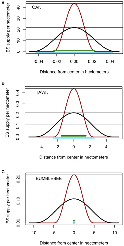
Figure 2. Characteristics of the kernels and minimum intervention areas required and preempted by ES producing functional units. Two plausible kernel radii and two sizes of required intervention area are considered for each species. (A) Oaks, (B) Northern Harriers, (C) bumblebees. Black and burgundy lines represent the two kernels or proportion of one unit of ecosystem service per unit length as a function of distance to center. Thick horizontal green and blue lines represent the two amounts of landscape needed and preempted by each unit. Thin horizontal lines represent the three levels of average ES demand per unit landscape. Functional units are one tree for oaks, one nesting pair for Northern Harriers and one colony for bumblebees. Note the difference in the scales of the vertical and horizonal axes.

Northern Harrier Nesting Habitat in Integrated Grazing-Cropping Landscapes

Second, consider predation services provided by Northern (and Hen) Harriers (Circus hudsonius and Circus cyaneus). Northern Harriers are the only North American Harrier and although they are declining due to habitat loss, they still range in the whole section of North America NW of a line from Baja California to Halifax. These birds require nesting habitat consisting of meadows, wetlands and grasslands with low thick vegetation, and they hunt in widely open fields feeding mostly on voles, rats and other rodents. A few ha of lightly grazed grasslands may provide such habitat, particularly if patches are protected from grazing (Dechant et al., 2002). The intervention to promote this ES is the creation and protection of grassland patches with perching sites and undisturbed by grazing, tillage domestic animals or humans. Once a pair of birds establishes a nest, it defends and hunts in a territory that can range from 10 to 300 ha depending on the amount and quality of hunting habitat. Individuals can fly up to 100 km in a day and hunting territories can overlap depending on prey density (Massey et al., 2009). I explored two habitat radii (r_min = 1.5 and 2.5 hm) and two kernel radii (r_k = 2.5 and 5.0 hm) commensurate with literature values (Figure 2B). This represents an ES with an intermediate kernel/exclusion ratio ranging from 1 to 3.33. Average demand is set at 0.4375, 0.4375/2, or 0.4375/4 ES units per hectometer.

Bumblebee Colony and Habitat for Pollination Services

Last, consider pollination services provided by native eusocial bumblebees. Bumblebees (e.g., Bombus) are an important component of the pollinator guild that is threatened by lack of forage, land use change, parasites and diseases (Samuelson et al., 2018). These species are annual social species that grow in colonies by first having a stage with cohorts of workers and then switching to producing queens and males that disperse while the remaining workers and queen survive (Crone and Williams, 2016). These bees require nesting habitat without tillage or mowing where there is grass and dead plant material providing cavities such as old bird and rodent nests. Bees do not defend territories, and each nest requires just a few square meters of habitat with protection from predators. The intervention can be thought of as the creation of patches or protective vegetation and nectar rich flowers where we place nest boxes with starter bee colonies. Each colony can grow to have 50–500 workers that feed up to 2 km from the nest, but most activity is within a few hundred m (Thomson, 2004; Goulson, 2010). Two minimum habitat radii (r_min = 0.1 and 0.2 hm) and two kernel radii (r_k = 5 and 10 hm) were simulated (Figure 2C). This represents a FU with an extremely high ratio of kernel to minimum radius (r_k:r_min) ranging from 25 to 100.

Results

Percentage of demand met increased with increasing proportion of the landscape represented by the intervention, and the slope decreased with increasing landscape demand (Figures 3–5). In all cases simulated, percentage of demand met increases in a stair-step fashion where the steps represent the amount of intervention required for one additional ES producing unit to be established. Steps are not clearly visible in some graphs because they are small relative to the graph resolution. The lowest proportion of demand was met in the oak restoration with the highest demand, when the kernel radius and the minimum intervention radius r_min were similar (Figure 3L). Conversely, 100% of the demand for bumblebee pollination services was achieved with 2.5% of the landscape used for nesting and cover, when kernel radius (10 hm) was 100 times the minimum intervention radius and demand was just ½ of the kernel maximum, K(0) (Figure 5G).

FIGURE 3

Figure 3. Soil organic matter and quality services provided by oaks as a function of proportion of landscape that receives intervention, ES demand (columns), supply kernel (r_k), and exclusion (r_min) radii (rows), and distribution of interventions. Intervention consist of planting oaks. Blue lines represent interventions spread out evenly over the landscape; red lines represent interventions in a compact area in the center of the landscape. Except for (G), the red lines are behind the blue lines. Labels (A–L) refer to the combinations of ES demand, supply kernel radius and exclusion radius indicated on the columns and rows of the figure grid.

FIGURE 4

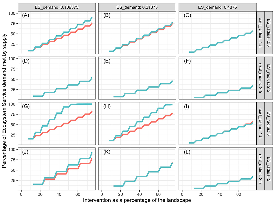
Figure 4. Predation services provided by Northern Harriers as a function of proportion of landscape that receives intervention, ES demand (columns), supply kernel radius and exclusion radius (rows), and distribution of intervention. The intervention is the creation of nesting habitat with tall bunchgrasses and perching sites that are undisturbed by human or domestic animal activity. Blue lines represent interventions spread out evenly over the landscape; red lines represent the case when the intervention is performed as a compact area in the center of the landscape. Some blue lines cover the red lines. Labels (A–L) refer to the combinations of ES demand, supply kernel radius and exclusion radius indicated on the columns and rows of the figure grid.

FIGURE 5

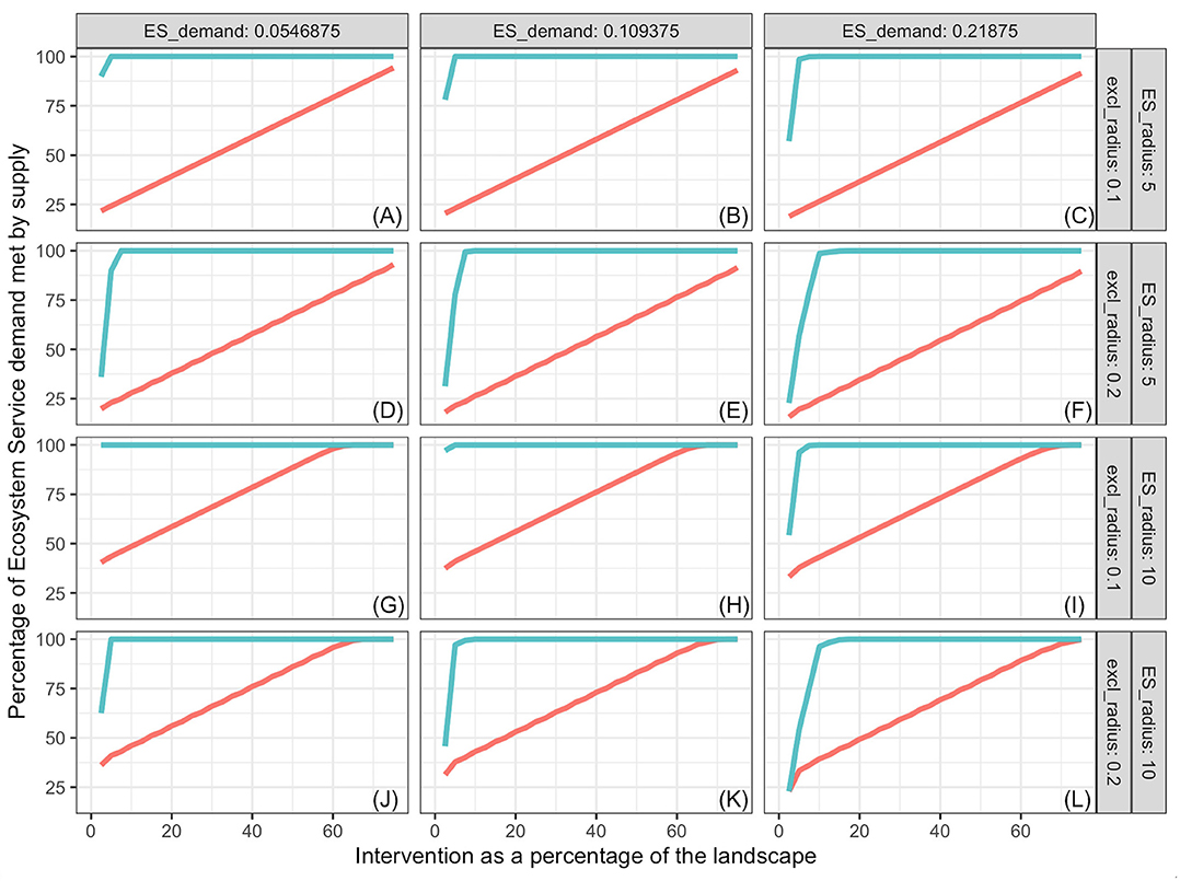
Figure 5. Pollination services provided by bumblebees as a function of proportion of landscape that receives intervention, ES demand (columns), supply kernel radius and exclusion radius (rows), and distribution of interventions. The intervention is creation of nesting habitat and introduction of foundation colonies of bumblebees. Blue lines represent interventions spread out evenly over the landscape; red lines represent results when all the intervention is performed as a compact area in the center of the landscape. Some blue lines cover the red lines. Labels (A–L) refer to the combinations of ES demand, supply kernel radius and exclusion radius indicated on the columns and rows of the figure grid.

In general, more ES demand was met when the intervention was spread out in the landscape (blue lines) than when it was in a single compact block (red lines). However, there were significant high-order interactions among all factors. The advantage of spread out over compact intervention distribution decreased as the exclusion radius increased and increased with increasing kernel radius within ES type (soil improvement by oaks, population regulation by Northern Harriers or pollination by bumblebee). The size of this 2-way interaction depended on the level of demand. For interventions with exclusion radius commensurate with the ES kernel radius (Figures 3A–C,J–L, 4D–F), the advantage of spreading the intervention was nil.

Both for oaks and Northern Harriers, the proportion of demand met at any level of intervention declined as average demand per unit landscape increased. This is a consequence of the low kernel:exclusion ratio, which prevents the “stacking” of service supply from many centers. When demand of ES per unit landscape is high relative to the kernel scale, it is impossible to meet a large proportion of the demand unless services provided by different units are additive and units can be packed densely enough. The maximum packing density is limited by the exclusion distance or amount of landscape that is preempted by each unit. In the case of bumblebees, the packing is not limited because multiple colonies can be established close to each other relative to the reach of their supply kernel.

Considering all results together, the most dramatic differences appear among species, although all three examples fall under the class of “ES proximity” defined by Syrbe and Grunewald (2017). On one extreme, oak restoration effects on soil organic matter are limited -relative to the maximum achieved at the tree center- because the benefits do not extend much beyond the tree canopy, and canopy overlap is not allowed. These conditions practically eliminate the effects of tree spatial distribution on the total demand met. On the other extreme, establishment of bumblebee colonies evenly spread in the landscape saturate the demand with very small proportions of landscape used for the colonies. Each new colony preempts a very small fraction of landscape but extends services over a large distance. When colonies are packed in a compact central intervention patch, the proportion of demand met increases linearly with proportion of landscape under intervention, and the slope is only slightly affected by other factors.

Proportion of demand met tended to decrease when the distribution of demand is concentrated in patches instead of being uniformly spread (not shown in figures). This effect happens because a concentrated demand is more likely to exceed local supply, and therefore it is stronger when kernel distance is limited by long exclusion distances, and when spatial exclusion prevents the stacking of kernels.

If interactions among ES supplying units (nesting pair of Northern Harriers, bee colonies, individual trees) are highly interferential and limit the total supply at any point to be that supplied by a single unit (Equation 3), proportion of demand met is reduced, particularly when demand per area is high relative to the maximum that a single unit can provide (Figure 6). For example, when “local” bumblebees prevent members of other colonies from foraging in the territory near the “local” colony, and demand per area is twice the maximum a colony can provide, a maximum of 50% of the demand would be met (Figure 6C). The negative effects of exclusive territory use beyond the minimum intervention area needed per FU (r_min) declines to almost nothing when the ratio of kernel to r_min declines to 3 or less. Highly territorial organisms with territories much larger than the minimum intervention needed for establishment (r_min) are inefficient ES providers unless demand density is much lower than what each FU can provide.

FIGURE 6

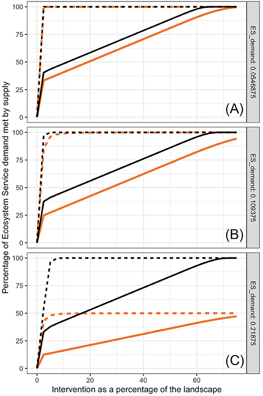
Figure 6. Hypothetical effects of interactions between ES producing units on proportion of ES demand met. Black lines represent the same cases of bumblebees in (Figures 4G–I). Orange lines represent what would happen if supply of services equals the value provided by the nearest kernel (bee colony) only. Solid lines are for compact distribution of intervention and dashed lines are for evenly distributed patches, each with size equal to the minimum needed to establish a colony.

Discussion

A model of supply and demand of ecosystem services that takes into account the distribution of services around the central locations of ES producing units shows that the efficiency with which ES demand is met depends strongly on the spatial distribution of the units and the relationship between the size of service producing area and service benefitting area, which is inherent to the service and the specific organism, population or community providing the service. This modeling framework borrows heavily from ecological field theory (Walker et al., 1989) whereby plant interactions are represented by the overlap of individual domains of influence. Field intensity declines with distance from the plant center according to various response types. In the simulations I present, the ecosystem service kernel represents the ecological field and the exclusion radius represents the actual space occupied or preempted by the plant or other ES producing unit.

Ecological functions or effects that decline with distance to a central place in a kernel-like fashion have been described for many organisms. I think that effects that decline with distance are a result of the fact that effects must involve flows of matter, energy, or information (which actually is in energy or matter) (Cadenasso et al., 2003), and resistance to flows, signal degradation and dilution increase with distance. Effects that do not decline quasi-exponentially with increasing distance require specific processes and inputs of energy to reverse the tendency. For example, (1) concentrations of soil organic matter and extractable nutrients decline, and soil temperatures increase in a curvilinear fashion with increasing distance to the trunk of Acacia tortilis trees in a Kenyan savanna (Belsky et al., 1989); (2) seed dispersal depends on height of seed release and declines steeply with distance to mother plant (Davies and Sheley, 2007); (3) vole herbivory damage to tree seedlings declines with increasing distance to forest edge (Cadenasso and Pickett, 2000); (4) centrifugal (or centripetal, depending on species) redistribution of rainfall by tree canopies increases with distance to the tree (Frischbier and Wagner, 2015).

The model is applied to three specific examples of ecosystem services, but how general is the approach? The three examples (carbon sequestration and soil OM provided by oaks, pollination services provided by bumblebees and predation services provided by Northern Harriers) are biotic regulation and maintenance services, according to the Common International Classification of Ecosystem Services (CICES) V5.1 (Haines-Young and Potschin, 2018). Strictly, carbon sequestration is not an ecosystem service, but it can be used as a proxy for the regulating effect it can have on the atmosphere. I do not propose a relationship between the class of ES and the applicability of the model, because ES classifications [reviewed by Czúcz et al. (2018)] seem to be based more on type of function (provisioning, regulation, cultural) whereas the model I describe focuses on relationships between spatial scales of interventions and the ES affected by those interventions. I did not select the interventions and ES analyzed on the basis of the class of ES, but to represent contrasting scales of ecological fields. For example, the analysis would be different for the oak interventions if the focal ES were aesthetic value, which has a much larger kernel than that for soil organic matter. Thus, at least in principle, the approach is general and not restricted to specific types of ES. Any intervention and related ES can be subjected to the analysis proposed, but of course, the feasibility of interventions and the effectiveness of the ES will depend on the specific situation considered.

Kernel and Exclusion Radius

The ratio kernel:exclusion radius is a dimensionless metric of the effectiveness of functional units to provide ES beyond interventions. For the organisms and services considered here, it makes sense that the exclusion radius is smaller than the kernel radius. The area over which the service is supplied extends well-beyond the space occupied and preempted by each ES producing unit. However, in the case of plant and soil services, the exclusion and kernel radii can be very similar, because most processes that involve herbaceous plants and their soil involve movement over short distances. The FU kernel could be smaller than the space occupied by the unit, for example if the ES responds in a highly non-linear manner to the action of a FU, with a positive threshold.

Ecosystem service kernels do not have to be constant for each ES producing unit but can adapt to the context. Wu et al. (1985) provide a modeling framework for temporally variable ecological fields of water and nutrients for plants. Mobile and adaptable predator like a Northern Harrier can adjust its hunting range and territory size depending on demand (prey density) and Northern Harrier population density (Norman and Jones, 1984; Jenner et al., 2011; Valeix et al., 2012; Kittle et al., 2015). Unlike what I simulated, Northern Harriers can expand their territory when prey density is low and contract it when it is high or when there are competitors nearby. It is possible that in all cases, the whole unit of ES service is provided within the modified kernel, and thus, the negative effects of increasing demand or competition on proportion of demand met would be mitigated. Species with adaptable kernels would be more efficient at meeting ES demand and less susceptible to the effects of spatial distribution of interventions than what is shown in the simulations I present. I expect that organisms that are mobile, fast relative to their range and lifespan, and with better mechanisms to gather and store information, are more likely to exhibit more dynamically adaptable kernels.

Spatial Distribution of Interventions

Results show that in general, spreading the intervention increases the effectiveness of ES supply relative to compact intervention areas. However, these results are completely dependent on the fact that the intervention was spread out into patches that were of radius equal to the exclusion or minimal radius of intervention necessary for one ES producing unit (nest, colony, plant). In fact, the spatial distribution of intervention areas can be managed to promote services of a specific kind and scale.

This conceptual framework to manage supply of ES can be extended by considering the spatial distribution of interventions across a large range of resolutions in relation to the “salient” or inherent scales at which FUs operate or integrate their environment. In general, larger and longer-lived organisms integrate resources over larger spaces and longer times, but there are notable exceptions. For example, individual bumblebees and even whole colonies are very small and short lived relative to the large areas over which they forage. Up to this point, interventions have been considered to be convex spatial extensions where all points inside an intervention patch receive the intervention. We can consider other feasible spatial distributions of interventions where resource density depends on the scale of analysis (Milne et al., 1992; Ritchie, 1998). For example, consider the seeding of native bunchgrasses as an intervention to create habitat for Northern Harriers. Areas can be drill seeded with various distances between rows, thus changing the grain of the intervention. From the Northern Harrier's point of view, which integrates information at a large scale, areas planted with rows that are 1 m apart are likely perceived as suitable nesting habitat. Conversely, the same grassland is perceived as alternating bands of suitable and unsuitable habitat by small organisms (say aphids and ladybugs) that live on the surface of the grass. Reducing the distance of rows to 0.5 m will not change the amount of Northern Harrier habitat, but it will potentially double the habitat area for aphids and ladybugs.

Further, consider the same amount of an intervention that can be used both for bumblebee and Northern Harrier nesting habitat. If the intervention is spread out into patches smaller than those needed for bumblebee habitat and far enough from each other that they are perceived as separate patches by both species, the intervention will generate neither pollination nor predation services. The same amount of intervention could be applied in separate patches of sufficient size as in the bumblebee simulations, thus generating abundant pollination but no predation services. Further increases in patch size or reductions in distance between patches would accomplish both services. Densely packed patches, each too small for bumblebees, could constitute Northern Harrier habitat, thus providing only predation services. By using designed spatial distributions of interventions with fractal-like properties, it may be possible to promote different compositions of ES supply by creating patchiness at multiple species and function-specific scales.

Ritchie and Olff (1999) showed that the fractal nature of habitat, food and resources frequently observed in nature can explain patterns of diversity. Species that use the same resources but that differ in size need to use different patches because of the relationship between their requirements and the resolutions at which they perceive and explore their habitat. Simply put, larger species require large patches with lower concentration of resources than smaller ones (Laca et al., 2010; Sensenig et al., 2010). Foragers have specific foraging scales, the size of the space searched for food at any instant in time (Ritchie, 1998), and the resolution with which they search for resources needs to balance the rates at which they acquire and spend resources. The idea can be extended to resources other than those contained in food, such as nesting locations. The present model applies the concepts presented by Ritchie and Olff (1999) in reverse: instead of using them to explain patterns of diversity as a function of natural spatial patterns of resources, I propose that spatial patterns of interventions can be used to promote specific patterns of community composition that provide the ES demanded.

Obviously, control of spatial distribution of interventions is not a new concept, but my claim is that its potential has barely been tapped. For example, intercropping has probably been used for millennia, and it has a prominent place for the sustainable intensification of agriculture. A recent global meta-analysis reveals that on average intercrops produce 38% more gross energy and 33% more gross incomes using 23% less land (Martin-Guay et al., 2018). Multiple ecological functions and interactions are likely to be involved in the greater efficiency of intercrops, such as niche complementarity, temporal niche differentiation (Yu et al., 2015), biodiversity of natural enemies, demographic limitation on pest populations, mutualism and microenvironmental modification. All of these have a spatial nature that can be thought of as kernels of influence with a variety of dynamic extents. Whereas, Martin-Guay et al. (2018) did not detect effects of spatial distribution of crop species (“intercropping pattern”: rows, strips or mixed) on the land equivalent ratio (a measure of overall intercropping advantage), Yu et al. (2015) found a significant gradient where the land equivalent ratio of intercropping increased gradually from mixed to row to strips. In any case, and aside from the uncertainty implicit in failure to statistically detect differences, the lack of effects of intercropping pattern has to be taken within the context that there was a clear difference between sole crops and intercropping. The point is that “sole” crops differ from intercropping by the distance between the species. There must be a strip width (i.e., degree of interspersion or more generally, spatial pattern) at which intercropping becomes adjacent sole crops. Thus, the difference found between intercropping and monoculture cropping implies an effect of spatial distribution of the component crops. Industrialization of agriculture has taken us in the path of large uniform monoculture fields, with all the commensurate specializations in mechanization, distribution and marketing cultures that make change difficult. But imagine the potential to sustainably increase the production of multiple ecosystem services by creating agro-ecological landscapes where spatial distributions of seeding interventions are tailored to provide what is demanded. I surmise that research in this area has been constrained by the scales of technology, but as “precision” technology continues to develop, need and opportunities for research on spatial interactions and effects across a continuum of scales will increase.

In practice, the best amount and spatial distribution of interventions is determined by many factors beyond the spatial ecology of organisms and functions involved in the creation and delivery of ES. Opportunity and cost are probably two of the most important factors that weigh in to determine a good allocation of interventions. In some cases, costs will increase with the complexity of the spatial distribution of interventions. For example, setting up and maintaining multiple bumblebee nests in a single large patch is easier and cheaper than spreading them evenly over the extent of an orchard. As a matter of fact, domestic bee colonies are usually managed in large groups that result in less than optimal pollination over the whole orchard. Cunningham et al. (2016) clearly showed that in spite of the ability to fly and forage over long distances, pollination activity declines dramatically with distance to the colony, and that for a given overall density of colonies, a more uniform distribution of colonies leads to increased pollination and fruit set. For a given landscape-level density of colonies per ha, the optimal combination of number of colonies per placement and distance between placements is the one for which the cost of adding one placement equals the gains from the additional fruit set achieved.

Humans and institutions are crucial agents in the organization and function of landscapes. People and institutions create demand, set prices, generate and distribute information, create, manage and modify spatial distribution channels. Decisions by individuals, groups and institutions, just like ecological functions, have specific reaches and spatial distributions. One problem may be a disconnect between the reach of agent's decisions, or the reach of the information used for agent decisions, and the spatial characteristics of the functions affected. For example, Inogwabini (2020) wrote:

“It is here, in describing spatial functions that conservation has its entire place; not only because within the landscapes there are protected areas but also because each functional space should have a mode of usage that will integrate the principle of durability. Land use becomes, therefore, a means through which to integrate conservation and sustainable livelihood. However, one needs to acknowledge that we are in a human-dominated landscape. That means conservation stakeholders had to evaluate not only the viability of proposed zoning and their effects on biodiversity across this large spatial scale, but also to project ecological, social, and economic influences that would alter the equilibrium of interactions between human and biological diversity across the landscape in a long-term perspective.”

The topic of spatial distribution of interventions is related to and might inform the land sharing vs. land sparing framework. I offer these comments with caution, because the sharing vs. sparing debate is vastly more general and complex than the specific model for quantification of matched ES demand I present in this work. Moreover, the sharing-sparing debate is primarily focused on food production, whereas I focus on the supply of ES demanded. Phalan (2018) wrote:

“The land sparing-sharing framework originated as a model for quantifying and understanding the implications for wild species of using land in different ways to produce food. It is based on the idea that there are two main ways to reduce the impacts of farming on wild species—making farmland itself more wildlife-friendly, or making more space for unfarmed habitats—and on the observation that there is a tension between these two sorts of interventions.”

The present model and approach do not inherently imply any support for either extreme of the “sparing-sharing” debate, but they align almost completely with the concept of “multiple-scale land sparing” where food production and conservation of wild species is approached through a strategy of nested hierarchical scales of actions and ecological functions (Ekroos et al., 2016). Based on the concepts of spatial and temporal scales presented in this work, at least part of the difference between sparing and sharing is a difference in scale. Simply put, sparing could be seen as sharing with a very large grain, where the intervention is the protection of areas of natural habitat. Under the reasonable assumption that most if not all species are related to the production of some ES, sparing can also be seen as interventions applied to promote the services provided by species that require large exclusion radius and have a kernel:exclusion radius ratio close to 1.

Conclusion

Although I only explored the effects of spatial distributions of interventions, the concepts are easily extended to the space-time continuum (e.g., Wu et al., 1985). Interventions with various durations might be distributed independently over space and time. The specific effects of each distribution on ecosystem services and multiple functions in interspersed agricultural, wild and urban landscapes can be surprisingly non-linear and counterintuitive, even when just a few simple mechanisms are involved, as I show in this work. Simultaneous manipulation of many of the dimensions of spatio-temporal distributions of interventions at the appropriate scales opens a myriad of management options in the search for sustainable landscapes.

Data Availability Statement

The original contributions presented in the study are included in the article/supplementary material, further inquiries can be directed to the corresponding author.

Author Contributions

The author confirms being the sole contributor of this work and has approved it for publication.

Funding

This work was partially funded by Grant number USDA-NIFA, Rangeland Research Program Grant #CA-D-PLS-2119-CG to EAL.

Conflict of Interest

The author declares that the research was conducted in the absence of any commercial or financial relationships that could be construed as a potential conflict of interest.

References

Bagstad, K. J., Johnson, G. W., Voigt, B., and Villa, F. (2013). Spatial dynamics of ecosystem service flows: a comprehensive approach to quantifying actual services. Ecosyst. Serv. 4, 117–125. doi: 10.1016/j.ecoser.2012.07.012

CrossRef Full Text | Google Scholar

Belsky, A. J., Amundson, R. G., Duxbury, J. M., Riha, S. J., Ali, A. R., and Mwonga, S. M. (1989). The effects of trees on their physical, chemical and biological environments in a semi-arid Savanna in Kenya. J. Appl. Ecol. 26, 1005–1024. doi: 10.2307/2403708

CrossRef Full Text | Google Scholar

Brudvig, L. A., and Asbjornsen, H. (2008). Patterns of oak regeneration in a Midwestern savanna restoration experiment. For. Ecol. Manage. 25, 3019–3025. doi: 10.1016/j.foreco.2007.11.017

CrossRef Full Text | Google Scholar

Cadenasso, M. L., and Pickett, S. T. A. (2000). Linking forest edge structure to edge function: mediation of herbivore damage. J. Ecol. 88, 31–44. doi: 10.1046/j.1365-2745.2000.00423.x

CrossRef Full Text | Google Scholar

Cadenasso, M. L., Pickett, S. T. A., Weathers, K. C., and Jones, C. G. (2003). A framework for a theory of ecological boundaries. Bioscience. 53, 750–758. doi: 10.1641/0006-3568(2003)053[0750:AFFATO]2.0.CO;2

CrossRef Full Text | Google Scholar

Crone, E. E., and Williams, N. M. (2016). Bumble bee colony dynamics: quantifying the importance of land use and floral resources for colony growth and queen production. Ecol. Lett. 19, 460–468. doi: 10.1111/ele.12581

PubMed Abstract | CrossRef Full Text | Google Scholar

Cunningham, S. A., Fournier, A., Neave, M. J., and Le Feuvre, D. (2016). Improving spatial arrangement of honeybee colonies to avoid pollination shortfall and depressed fruit set. J. Appl. Ecol. 53, 350–359. doi: 10.1111/1365-2664.12573

CrossRef Full Text | Google Scholar

Czúcz, B., Arany, I., Potschin-Young, M., Bereczki, K., Kertész, M., Kiss, M., et al. (2018). Where concepts meet the real world: a systematic review of ecosystem service indicators and their classification using CICES. Ecosyst. Serv. 29, 145–157. doi: 10.1016/j.ecoser.2017.11.018

CrossRef Full Text | Google Scholar

Dahlgren, R. A., Horwath, W. R., Tate, K. W., and Camping, T. J. (2003). Blue oak enhance soil quality in California oak woodlands. Calif. Agric. 57, 42–47. doi: 10.3733/ca.v057n02p42

CrossRef Full Text | Google Scholar

Davies, K. W., and Sheley, R. L. (2007). Influence of neighboring vegetation height on seed dispersal: implications for invasive plant management. Weed Sci. 55, 626–630. doi: 10.1614/WS-07-067.1

CrossRef Full Text | Google Scholar

Dechant, J. A., Sondreal, M. L., Johnson, D. H., Igl, L. D., Goldade, C. M., Nenneman, M. P., et al. (2002). Effects of Management Practices on Grassland Birds: Northern Harrier. Reston, VA: USGS Northern Prairie Wildlife Research Center.

Google Scholar

Ekroos, J., Ödman, A. M., Andersson, G. K. S., Birkhofer, K., Herbertsson, L., Klatt, B. K., et al. (2016). Sparing land for biodiversity at multiple spatial scales. Front. Ecol. Evol. 3:145. doi: 10.3389/fevo.2015.00145

CrossRef Full Text | Google Scholar

Engemann, K., Pedersen, C. B., Arge, L., Tsirogiannis, C., Mortensen, P. B., and Svenning, J. C. (2019). Residential green space in childhood is associated with lower risk of psychiatric disorders from adolescence into adulthood. Proc. Natl. Acad. Sci. U. S. A. 116, 5188–5193. doi: 10.1073/pnas.1807504116

PubMed Abstract | CrossRef Full Text | Google Scholar

Frischbier, N., and Wagner, S. (2015). Detection, quantification and modelling of small-scale lateral translocation of throughfall in tree crowns of European beech (Fagus sylvatica L.) and Norway spruce (Picea abies (L.) Karst.). J. Hydrol. 522, 228–238. doi: 10.1016/j.jhydrol.2014.12.034

CrossRef Full Text | Google Scholar

Frost, W. E., and Edinger, S. B. (1991). Effects of tree canopies on soil characteristics of annual rangeland. J. Range Manage. 44, 286–288. doi: 10.2307/4002959

CrossRef Full Text | Google Scholar

Gill, R. A., and Burke, I. C. (1999). Ecosystem consequences of plant life form changes at three sites in the semiarid United States. Oecologia 121, 551–563. doi: 10.1007/s004420050962

PubMed Abstract | CrossRef Full Text | Google Scholar

Goulson, D. (2010). Bumblebees : Behaviour, Ecology, and Conservation. 2nd Edn. Oxford; New York, NY: Oxford UP. Print. Oxford Biology.

Google Scholar

Haines-Young, R., and Potschin, M. B. (2018). Common International Classification of Ecosystem Services (CICES) V5.1 and Guidance on the Application of the Revised Structure. Available online at: www.cices.eu. (accessed November 20, 2020). doi: 10.3897/oneeco.3.e27108

CrossRef Full Text | Google Scholar

Inogwabini, B.-I. (2020). “Landscape: re-assessing the conservation paradigm,” in Reconciling Human Needs and Conserving Biodiversity: Large Landscapes as a New Conservation Paradigm: The Lake Tumba, Democratic Republic of Congo, ed B.-I. Inogwabini (Cham: Springer), 17–28. doi: 10.1007/978-3-030-38728-0_2

CrossRef Full Text | Google Scholar

Jenner, N., Groombridge, J., and Funk, S. M. (2011). Commuting, territoriality and variation in group and territory size in a black-backed jackal population reliant on a clumped, abundant food resource in Namibia. J. Zool. 284, 231–238. doi: 10.1111/j.1469-7998.2011.00811.x

CrossRef Full Text | Google Scholar

Kittle, A. M., Anderson, M., Avgar, T., Baker, J. A., Brown, G. S., Hagens, J., et al. (2015). Wolves adapt territory size, not pack size to local habitat quality. J. Anim. Ecol. 84, 1177–1186. doi: 10.1111/1365-2656.12366

PubMed Abstract | CrossRef Full Text | Google Scholar

Laca, E. A., Sokolow, S., Galli, J. R., and Cangiano, C. A. (2010). Allometry and spatial scales of foraging in mammalian herbivores. Ecol. Lett. 13, 311–320. doi: 10.1111/j.1461-0248.2009.01423.x

PubMed Abstract | CrossRef Full Text | Google Scholar

Lindborg, R. L. J., Gordon, R., Malinga, J., Bengtsson, G., Peterson, R., Bommarco, L., et al. (2017). How spatial scale shapes the generation and management of multiple ecosystem services. Ecosphere 8:e01741. doi: 10.1002/ecs2.1741

CrossRef Full Text | Google Scholar

Liu, Y., Bi, J., Lv, J., Ma, Z., and Wang, C. (2017). Spatial multi-scale relationships of ecosystem services: a case study using a geostatistical methodology. Sci. Rep. 7:9486. doi: 10.1038/s41598-017-09863-1

PubMed Abstract | CrossRef Full Text | Google Scholar

Marañón, T., Pugnaire, F. I., and Callaway, R. M. (2009). Mediterranean-climate oak savannas: the interplay between abiotic environment and species interactions. Web Ecol. 9, 30–43. doi: 10.5194/we-9-30-2009

CrossRef Full Text | Google Scholar

Martin-Guay, M. O., Paquette, A., Dupras, J., and Rivest, D. (2018). The new Green Revolution: sustainable intensification of agriculture by intercropping. Sci. Total Environ. 615, 767–772. doi: 10.1016/j.scitotenv.2017.10.024

PubMed Abstract | CrossRef Full Text | Google Scholar

Massey, B. H., Griffin, C. R., and McGarigal, K. (2009). Habitat use by foraging Northern Harriers on Nantucket Island, Massachusetts. Wilson J. Ornithol. 121, 765–769. doi: 10.1676/09-015.1

CrossRef Full Text | Google Scholar

Milne, B. T., Turner, M. G., Wiens, J. A., and Johnson, A. R. (1992). Interactions between the fractal geometry of landscapes and allometric herbivory. Theor. Popul. Biol. 41, 337–353. doi: 10.1016/0040-5809(92)90033-P

CrossRef Full Text | Google Scholar

Norman, M. D., and Jones, G. P. (1984). Determinants of territory size in the pomacentrid reef fish, Parma victoriae. Oecologia 61, 60–69. doi: 10.1007/BF00379090

PubMed Abstract | CrossRef Full Text | Google Scholar

Phalan, B. T. (2018). What have we learned from the land sparing-sharing model? Sustainability 10:1760. doi: 10.3390/su10061760

CrossRef Full Text | Google Scholar

Ritchie, M. E. (1998). Scale-dependent foraging and patch choice in fractal environments. Evol. Ecol. 12, 309–330. doi: 10.1023/A:1006552200746

CrossRef Full Text | Google Scholar

Ritchie, M. E., and Olff, H. (1999). Spatial scaling laws yield a synthetic theory of biodiversity. Nature 400, 557–560. doi: 10.1038/23010

PubMed Abstract | CrossRef Full Text | Google Scholar

Sala, O. E., Yahdjian, L., Havstad, K., and Aguiar, M. R. (2017). “Rangeland ecosystem services: nature's supply and humans' demand,” in Rangeland Systems. Springer Series on Environmental Management, ed D. Briske (Cham: Springer), 467–489. doi: 10.1007/978-3-319-46709-2_14

CrossRef Full Text | Google Scholar

Samuelson, A. E., Gill, R. J., Brown, M. J. F., and Leadbeater, E. (2018). Lower bumblebee colony reproductive success in agricultural compared with urban environments. Proc. R. Soc. B Biol. Sci. 285:20180807. doi: 10.1098/rspb.2018.0807

PubMed Abstract | CrossRef Full Text | Google Scholar

Sensenig, R. L., Demment, M. W., and Laca, E. A. (2010). Allometric scaling predicts preferences for burned patches in a guild of East African grazers. Ecology 91, 2898–2907. doi: 10.1890/09-1673.1

PubMed Abstract | CrossRef Full Text | Google Scholar

Syrbe, R. U., and Grunewald, K. (2017). Ecosystem service supply and demand–the challenge to balance spatial mismatches. Int. J. Biodivers. Sci. Ecosyst. Serv. Manag. 13, 148–161. doi: 10.1080/21513732.2017.1407362

CrossRef Full Text | Google Scholar

Thomson, D. (2004). Competitive interactions between the invasive European honey bee and native bumble bees. Ecology 85, 458–470. doi: 10.1890/02-0626

CrossRef Full Text | Google Scholar

Valeix, M., Loveridge, A. J., and Macdonald, D. W. (2012). Influence of prey dispersion on territory and group size of African lions: a test of the resource dispersion hypothesis. Ecology 93, 2490–2496. doi: 10.1890/12-0018.1

PubMed Abstract | CrossRef Full Text | Google Scholar

Walker, J., Sharpe, P. J. H., Penridge, L. K., and Wu, H. (1989). Ecological field theory - the concept and field tests. Vegetatio 83, 81–95. doi: 10.1007/BF00031682

CrossRef Full Text | Google Scholar

Wu, H. I., Sharpe, P. J. H., Walker, J., and Penridge, L. K. (1985). Ecological field theory: a spatial analysis of resource interference among plants. Ecol. Modell. 29, 215–243. doi: 10.1016/0304-3800(85)90054-7

CrossRef Full Text | Google Scholar

Yahdjian, L., Sala, O. E., and Havstad, K. M. (2015). Rangeland ecosystem services: shifting focus from supply to reconciling supply and demand. Front. Ecol. Environ. 13, 44–51. doi: 10.1890/140156

CrossRef Full Text | Google Scholar

Yu, Y., Stomph, T. J., Makowski, D., and van der Werf, W. (2015). Temporal niche differentiation increases the land equivalent ratio of annual intercrops: a meta-analysis. Field Crops Res. 184, 133–144. doi: 10.1016/j.fcr.2015.09.010

CrossRef Full Text | Google Scholar