 Matthew Dixon
 Justin London
- 1Department of Applied Math, Illinois Institute of Technology, Chicago, IL, United States
- 2Stuart School of Business, Illinois Institute of Technology, Chicago, IL, United States
The era of modern financial data modeling seeks machine learning techniques which are suitable for noisy and non-stationary big data. We demonstrate how a general class of exponential smoothed recurrent neural networks (α-RNNs) are well suited to modeling dynamical systems arising in big data applications such as high frequency and algorithmic trading. Application of exponentially smoothed RNNs to minute level Bitcoin prices and CME futures tick data, highlight the efficacy of exponential smoothing for multi-step time series forecasting. Our α-RNNs are also compared with more complex, “black-box”, architectures such as GRUs and LSTMs and shown to provide comparable performance, but with far fewer model parameters and network complexity.
1. Introduction
Recurrent neural networks (RNNs) are the building blocks of modern sequential learning. RNNs use recurrent layers to capture non-linear temporal dependencies with a relatively small number of parameters (Graves, 2013). They learn temporal dynamics by mapping an input sequence to a hidden state sequence and outputs, via a recurrent layer and a feedforward layer.
There have been exhaustive empirical studies on the application of recurrent neural networks to prediction from financial time series data such as historical limit order book and price history (Borovykh et al., 2017; Dixon, 2018; Borovkova and Tsiamas, 2019; Chen and Ge, 2019; Mäkinen et al., 2019; Sirignano and Cont, 2019). Sirignano and Cont (2019) find evidence that stacking networks leads to superior performance on intra-day stock data combined with technical indicators, whereas (Bao et al., 2017) combine wavelet transforms and stacked autoencoders with LSTMs on OHLC bars and technical indicators. Borovykh et al. (2017) find evidence that dilated convolutional networks out-perform LSTMs on various indices. Dixon (2018) demonstrate that RNNs outperform feed-forward networks with lagged features on limit order book data.
There appears to be a chasm between the statistical modeling literature (see, e.g., Box and Jenkins 1976; Kirchgässner and Wolters 2007; Hamilton 1994) and the machine learning literature (see. e.g., Hochreiter and Schmidhuber 1997; Pascanu et al. 2012; Bayer 2015). One of the main contributions of this paper is to demonstrate how RNNs, and specifically a class of novel exponentially smoothed RNNs (α-RNNs), proposed in (Dixon, 2021), can be used in a financial time series modeling framework. In this framework, we rely on statistical diagnostics in combination with cross-validation to identify the best choice of architecture. These statistical tests characterize stationarity and memory cut-off length and provide insight into whether the data is suitable for longer-term forecasting and whether the model must be non-stationary.
In contrast to state-of-the-art RNNs such as LSTMs and Gated Recurrent Units (GRUs) (Chung et al., 2014), which were designed primarily for speech transcription, the proposed class of α-RNNs is designed for times series forecasting using numeric data. α-RNNs not only alleviate the gradient problem but are designed to i) require fewer parameters and numbers of recurrent units and considerably fewer samples to attain the same prediction accuracy1; ii) support both stationary and non-stationary times series2; and iii) be mathematically accessible and characterized in terms of well known concepts in classical time series modeling, rather than appealing to logic and circuit diagrams.
As a result, through simple analysis of the time series properties of α-RNNs, we show how the value of the smoothing parameter, α, directly characterizes its dynamical behavior and provides a model which is both more intuitive for time series modeling than GRUs and LSTMs while performing comparably. We argue that for time series modeling problems in finance, some of the more complicated components, such as reset gates and cell memory present in GRUs and LSTMs but absent in α-RNNs, may be redundant for our data. We exploit these properties in two ways i) first, we using a statistical test for stationarity to determine whether to deploy a static or dynamic α-RNN model; and ii) we are able to reduce the training time, memory requirements for storing the model, and in general expect α-RNN to be more accurate for shorter time series as they require less training data and are less prone to over-fitting. The latter is a point of practicality as many applications in finance are not necessarily big data problems, and the restrictive amount of data favors an architecture with fewer parameters to avoid over-fitting.
The remainder of this paper is outlined as follows. Section 2 introduces the static α-RNN. Section 3 bridges the time series modeling approach with RNNs to provide insight on the network properties. Section 4 introduces a dynamic version of the model and illustrates the dynamical behavior of α. Details of the training, implementation and experiments using financial data together with the results are presented in Section 5. Finally, Section 6 concludes with directions for future research.
2. α-RNNs
Given auto-correlated observations of covariates or predictors,
where
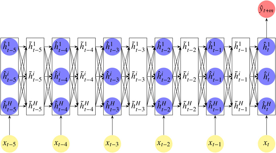
FIGURE 1. An illustrative example of an α-RNN with an alternating hidden recurrent layer (with blue nodes) and a smoothing layer (white block), “unfolded” over a sequence of six time steps. Each lagged feature
For each index in a sequence, s = t-p+2, … ,t, forward passes repeatedly update a hidden internal state
where
3. Univariate Times Series Modeling With Endogenous Features
This section bridges the time series modeling literature (Box and Jenkins, 1976; Kirchgässner and Wolters, 2007; Li and Zhu, 2020) and the machine learning literature. More precisely, we show the conditions under which plain RNNs are identical to autoregressive time series models and thus how RNNs generalize autoregressive models. Then we build on this result by applying time series analysis to characterize the behavior of static α-RNNs.
We shall assume here for ease of exposition that the time series data is univariate and the predictor is endogenous3, so that the data is
We find it instructive to show that plain RNNs are non-linear AR(p) models. For ease of exposition, consider the simplest case of a RNN with one hidden unit,
then
When the activation is the identity function
with geometrically decaying autoregressive coefficients when
The α-RNN(p) is almost identical to a plain RNN, but with an additional scalar smoothing parameter, α, which provides the recurrent network with “long-memory”4. To see this, let us consider a one-step ahead univariate α-RNN(p) in which the smoothing parameter is fixed and
This model augments the plain-RNN by replacing
We can easily verify this informally by simplifying the parameterization and considering the unactivated case. Setting
with the starting condition in each sequence,
and the model can be written in the simpler form
with auto-regressive weights
where we used the property that
4. Multivariate Dynamic α-RNNS
We now return to the more general multivariate setting as in Section 2. The extension of RNNs to dynamical time series models, suitable for non-stationary time series data, relies on dynamic exponential smoothing. This is a time dependent, convex, combination of the smoothed output,
where
Hence the smoothing can be viewed as a dynamic form of latent forecast error correction. When
where
4.1. Neural Network Exponential Smoothing
While the class of
This smoothing is a vectorized form of the above classical setting, only here we note that when
The hidden variable is given by the semi-affine transformation:
which in turn depends on the previous smoothed hidden variable. Substituting Eq. 13 into Eq. 12 gives a function of
We see that when
The challenge becomes how to determine dynamically how much error correction is needed. As in GRUs and LSTMs, we can address this problem by learning
5. Results
This section describes numerical experiments using financial time series data to evaluate the various RNN models. All models are implemented in v1.15.0 of TensorFlow (Abadi et al., 2016). Times series cross-validation is performed using separate training, validation and test sets. To preserve the time structure of the data and avoid look ahead bias, each set represents a contiguous sampling period with the test set containing the most recent observations. To prepare the training, validation and testing sets for m-step ahead prediction, we set the target variables (responses) to the
We use the SimpleRNN Keras method with the default settings to implement a fully connected RNN. Tanh activation functions are used for the hidden layer with the number of units found by time series cross-validation with five folds to be
Each architecture is trained for up to 2000 epochs with an Adam optimization algorithm with default parameter values and using a mini-batch size of 1,000 drawn from the training set. Early stopping is implemented using a Keras call back with a patience of 50 to 100 and a minimum loss delta between
5.1. Bitcoin Forecasting
One minute snapshots of USD denominated Bitcoin mid-prices are captured from Coinbase over the period from January 1 to November 10, 2018. We demonstrate how the different networks forecast Bitcoin prices using lagged observations of prices. The predictor in the training and the test set is normalized using the moments of the training data only so as to avoid look-ahead bias or introduce a bias in the test data. We accept the Null hypothesis of the augmented Dickey-Fuller test as we can not reject it at even the 90% confidence level. The data is therefore stationary (contains at least one unit root). The largest test statistic is
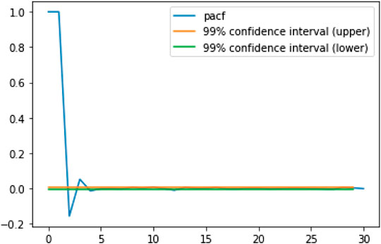
FIGURE 2. The partial autocorrelogram (PACF) for 1 min snapshots of Bitcoin mid-prices (USD) over the period January 1, 2018 to November 10, 2018.
We choose a sequence length of
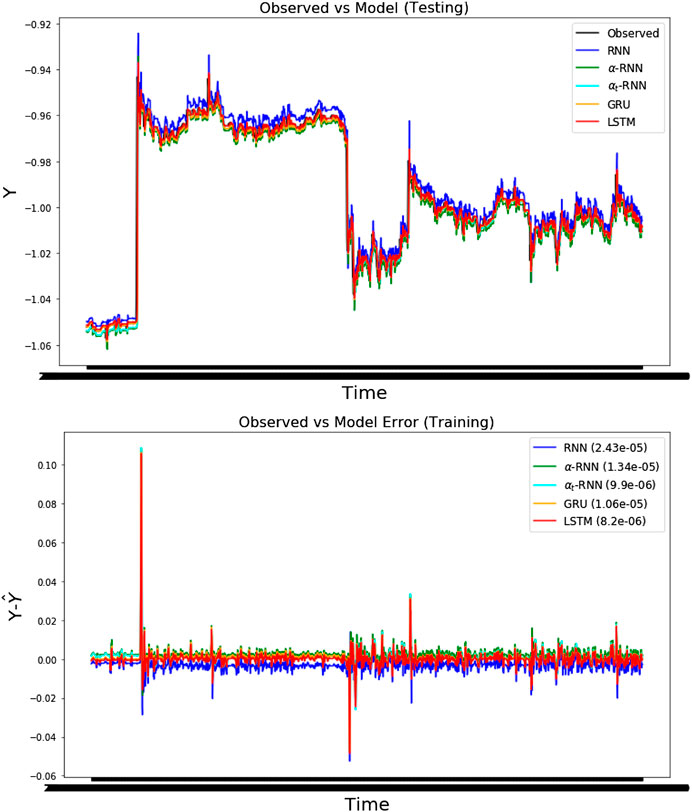
FIGURE 3. The four-step ahead forecasts of temperature using the minute snapshot Bitcoin prices (USD) with MSEs shown in parentheses. (top) The forecasts for each architecture and the observed out-of-sample time series. (bottom) The errors for each architecture over the same test period. Note that the prices have been standardized.
Viewing the results of time series cross validation, using the first 30,000 observations, in Table 1, we observe minor differences in the out-of-sample performance of the LSTM, GRU vs. the
TABLE 1. Thefour-stepahead Bitcoin forecasts are compared for various architectures using time series cross-validation. The half-life of the α-RNN is found to be 1.077 min (
5.2. High Frequency Trading Data
Our dataset consists of
We reject the Null hypothesis of the augmented Dickey-Fuller test at the 99% confidence level in favor of the alternative hypothesis that the data is stationary (contains no unit roots. See for example (Tsay, 2010) for a definition of unit roots and details of the Dickey-Fuller test). The test statistic is
The PACF in Figure 4 is observed to exhibit a cut-off at approximately 23 lags. We therefore choose a sequence length of
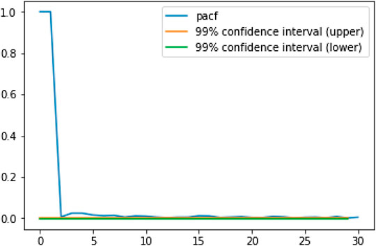
FIGURE 4. The PACF of the tick-by-tick VWAP of ESU6 over the month of August 2016.
Figure 5 compares the performance of the various networks and shows that plain RNN performs poorly, whereas and the
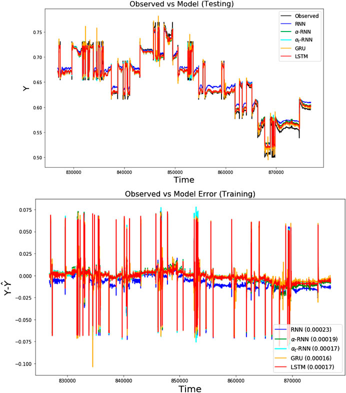
FIGURE 5. The ten-step ahead forecasts of VWAPs are compared for various architectures using the tick-by-tick dataset. (top) The forecasts for each architecture and the observed out-of-sample time series. (bottom) The errors for each architecture over the same test period.
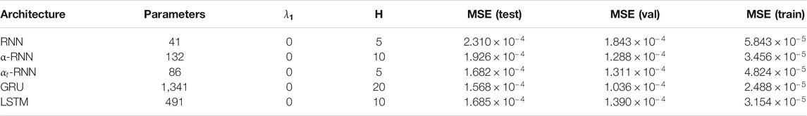
TABLE 2. Theten-stepahead forecasting models for VWAPs are compared for various architectures using time series cross-validation. The half-life of the α-RNN is found to be 2.398 periods (
6. Conclusion
Financial time series modeling has entered an era of unprecedented growth in the size and complexity of data which require new modeling methodologies. This paper demonstrates a general class of exponential smoothed recurrent neural networks (RNNs) which are well suited to modeling non-stationary dynamical systems arising in industrial applications such as algorithmic and high frequency trading. Application of exponentially smoothed RNNs to minute level Bitcoin prices and CME futures tick data demonstrates the efficacy of exponential smoothing for multi-step time series forecasting. These examples show that exponentially smoothed RNNs are well suited to forecasting, exhibiting few layers and needing fewer parameters, than more complex architectures such as GRUs and LSTMs, yet retaining the most important aspects needed for forecasting non-stationary series. These methods scale to large numbers of covariates and complex data. The experimental design and architectural parameters, such as the predictive horizon and model parameters, can be determined by simple statistical tests and diagnostics, without the need for extensive hyper-parameter optimization. Moreover, unlike traditional time series methods such as ARIMA models, these methods are shown to be unconditionally stable without the need to pre-process the data.
Data Availability Statement
The datasets and Python codes for this study can be found at https://github.com/mfrdixon/alpha-RNN.
Author Contributions
MD contributed the methodology and results, and JL contributed to the results section.
Funding
The authors declare that this study received funding from Intel Corporation. The funder was not involved in the study design, collection, analysis, interpretation of data, the writing of this article or the decision to submit it for publication.
Conflict of Interest
The authors declare that the research was conducted in the absence of any commercial or financial relationships that could be construed as a potential conflict of interest.
Appendix
1. GRUS and LSTMS1
1.1. GRUs
A GRU is given by:
When viewed as an extension of our
These additional layers (or cells) enable a GRU to learn extremely complex long-term temporal dynamics that a vanilla RNN is not capable of. Lastly, we comment in passing that in the GRU, as in a RNN, there is a final feedforward layer to transform the (smoothed) hidden state to a response:
1.2. LSTMs
LSTMs are similar to GRUs but have a separate (cell) memory,
The cell memory is updated by the following expression involving a forget gate,
In the terminology of LSTMs, the triple
When the forget gate,
The extra “memory”, treated as a hidden state and separate from the cell memory, is nothing more than a Hadamard product:
which is reset if
Thus the reset gate can entirely override the effect of the cell memory’s autoregressive structure, without erasing it. In contrast, the
The reset, forget, input and cell memory gates are updated by plain RNNs all depending on the hidden state
The LSTM separates out the long memory, stored in the cellular memory, but uses a copy of it, which may additionally be reset. Strictly speaking, the cellular memory has long-short autoregressive memory structure, so it would be misleading in the context of time series analysis to strictly discern the two memories as long and short (as the nomenclature suggests). The latter can be thought of as a truncated version of the former.
Footnotes
1Sample complexity bounds for RNNs have recently been derived by (Akpinar et al., 2019). Theorem 3.1 shows that for a recurrent units, inputs of length at most b, and a single real-valued output unit, the network requires only
2By contrast, plain RNNs model stationary time series, and GRUs/LSTMs model non-stationary, but no hybrid exists which provides the modeler with the control to deploy either.
3The sequence of features is from the same time series as the predictor hence
4Long memory refers to autoregressive memory beyond the sequence length. This is also sometimes referred to as “stateful”. For avoidance of doubt, we are not suggesting that the α-RNN has an additional cellular memory, as in LSTMs.
5The half-life is the number of lags needed for the coefficient
References
Abadi, M., Barham, P., Chen, J., Chen, Z., Davis, A., Dean, J., et al. (2016). “TensorFlow: a system for large-scale machine learning,” in Proceedings of the 12th USENIX conference on operating systems design and implementation, Savannah, GA, November 2–4, 2016 (Berkeley, CA: OSDI’16) 265–283.
Akpinar, N. J., Kratzwald, B., and Feuerriegel, S. (2019). Sample complexity bounds for recurrent neural networks with application to combinatorial graph problems. Preprint repository name [Preprint]. Available at: https://arxiv.org/abs/1901.10289.
Bao, W., Yue, J., and Rao, Y. (2017). A deep learning framework for financial time series using stacked autoencoders and long-short term memory. PloS One 12, e0180944–e0180924. doi:10.1371/journal.pone.0180944
Bayer, J. (2015). Learning sequence representations. MS dissertation. Munich, Germany: Technische Universität München.
Borovkova, S., and Tsiamas, I. (2019). An ensemble of LSTM neural networks for high‐frequency stock market classification. J. Forecast. 38, 600–619. doi:10.1002/for.2585
Borovykh, A., Bohte, S., and Oosterlee, C. W. (2017). Conditional time series forecasting with convolutional neural networks. Preprint repository name [Preprint]. Available at: https://arxiv.org/abs/1703.04691.
Box, G., and Jenkins, G. M. (1976). Time series analysis: forecasting and control. Hoboken, NJ: Holden Day, 575
Chen, S., and Ge, L. (2019). Exploring the attention mechanism in LSTM-based Hong Kong stock price movement prediction. Quant. Finance 19, 1507–1515. doi:10.1080/14697688.2019.1622287 \
Chung, J., Gülçehre, Ç., Cho, K., and Bengio, Y. (2014). Empirical evaluation of gated recurrent neural networks on sequence modeling. Preprint repository name [Preprint]. Available at: https://arxiv.org/abs/1412.3555.
Dixon, M. (2018). Sequence classification of the limit order book using recurrent neural networks. J. Comput. Sci. 24, 277. doi:10.1016/j.jocs.2017.08.018
Dixon, M. F., Polson, N. G., and Sokolov, V. O. (2019). Deep learning for spatio‐temporal modeling: dynamic traffic flows and high frequency trading. Appl. Stoch. Model. Bus Ind 35, 788–807. doi:10.1002/asmb.2399
Dixon, M. (2021). Industrial Forecasting with Exponentially Smoothed Recurrent Neural Networks, forthcoming in Technometrics.
Dixon, M., and London, J. (2021b). Alpha-RNN source code and data repository. Available at: https://github.com/mfrdixon/alpha-RNN.
Glorot, X., and Bengio, Y. (2010). “Understanding the difficulty of training deep feedforward neural networks,” in Proceedings of the international conference on artificial intelligence and statistics (AISTATS’10), Sardinia, Italy, Society for Artificial Intelligence and Statistics, 249–256
Graves, A (2013). Generating sequences with recurrent neural networks. Preprint repository name [Preprint]. Available at: https://arxiv.org/abs/1308.0850.
Hochreiter, S., and Schmidhuber, J. (1997). Long short-term memory. Neural. Comput. 9, 1735–1780. doi:10.1162/neco.1997.9.8.1735
Kirchgässner, G., and Wolters, J. (2007). Introduction to modern time series analysis. Berlin, Heidelberg: Springer-Verlag, 277
Li, D., and Zhu, K. (2020). Inference for asymmetric exponentially weighted moving average models. J. Time Ser. Anal. 41, 154–162. doi:10.1111/jtsa.12464
Mäkinen, Y., Kanniainen, J., Gabbouj, M., and Iosifidis, A. (2019). Forecasting jump arrivals in stock prices: new attention-based network architecture using limit order book data. Quant. Finance 19, 2033–2050. doi:10.1080/14697688.2019.1634277
Pascanu, R., Mikolov, T., and Bengio, Y. (2012). “On the difficulty of training recurrent neural networks,” in ICML’13: proceedings of the 30th international conference on machine learning, 1310–1318. Available at: https://dl.acm.org/doi/10.5555/3042817.3043083.
Sirignano, J., and Cont, R. (2019). Universal features of price formation in financial markets: perspectives from deep learning. Quant. Finance 19, 1449–1459. doi:10.1080/14697688.2019.1622295
Keywords: recurrent neural networks, exponential smoothing, bitcoin, time series modeling, high frequency trading
Citation: Dixon M and London J (2021) Financial Forecasting With α-RNNs: A Time Series Modeling Approach. Front. Appl. Math. Stat. 6:551138. doi: 10.3389/fams.2020.551138
Received: 12 April 2020; Accepted: 13 October 2020;
Published: 11 February 2021.
Edited by:
Glenn Fung, Independent Researcher, Madison, United StatesCopyright © 2021 Dixon and London. This is an open-access article distributed under the terms of the Creative Commons Attribution License (CC BY). The use, distribution or reproduction in other forums is permitted, provided the original author(s) and the copyright owner(s) are credited and that the original publication in this journal is cited, in accordance with accepted academic practice. No use, distribution or reproduction is permitted which does not comply with these terms.
*Correspondence: Matthew Dixon, bWF0dGhldy5kaXhvbkBpaXQuZWR1