 Zhouxuan Li
 Tao Xu
 Kai Zhang1
 Hong-Wen Deng
 Eric Boerwinkle
 Momiao Xiong
- 1School of Public Health, The University of Texas Health Science Center at Houston, Houston, TX, United States
- 2Tulane Center of Biomedical Informatics and Genomics, Deming Department of Medicine, School of Medicine, Tulane University, New Orleans, LA, United States
Given the lack of potential vaccines and effective medications, non-pharmaceutical interventions are the major option to curtail the spread of COVID-19. An accurate estimate of the potential impact of different non-pharmaceutical measures on containing, and identify risk factors influencing the spread of COVID-19 is crucial for planning the most effective interventions to curb the spread of COVID-19 and to reduce the deaths. Additive model-based bivariate causal discovery for scalar factors and multivariate Granger causality tests for time series factors are applied to the surveillance data of lab-confirmed Covid-19 cases in the US, University of Maryland Data (UMD) data, and Google mobility data from March 5, 2020 to August 25, 2020 in order to evaluate the contributions of social-biological factors, economics, the Google mobility indexes, and the rate of the virus test to the number of the new cases and number of deaths from COVID-19. We found that active cases/1,000 people, workplaces, tests done/1,000 people, imported COVID-19 cases, unemployment rate and unemployment claims/1,000 people, mobility trends for places of residence (residential), retail and test capacity were the popular significant risk factor for the new cases of COVID-19, and that active cases/1,000 people, workplaces, residential, unemployment rate, imported COVID cases, unemployment claims/1,000 people, transit stations, mobility trends (transit), tests done/1,000 people, grocery, testing capacity, retail, percentage of change in consumption, percentage of working from home were the popular significant risk factor for the deaths of COVID-19. We observed that no metrics showed significant evidence in mitigating the COVID-19 epidemic in FL and only a few metrics showed evidence in reducing the number of new cases of COVID-19 in AZ, NY and TX. Our results showed that the majority of non-pharmaceutical interventions had a large effect on slowing the transmission and reducing deaths, and that health interventions were still needed to contain COVID-19.
Introduction
As of August 25, 2020, the number of cumulative cases of COVID-19 in the US exceeded 5,727,107 and included 170,305, deaths (John Hopkins Coronavirus Resource Center, https://coronavirus.jhu.edu/MAP.HTML), thus causing a devastating public health and economic crisis. Since the number of new cases in the US remains high (36,339 in the US on August 25, 2020) ((John Hopkins Coronavirus Resource Center, https://coronavirus.jhu.edu/MAP.HTML), curbing the spread of COVID-19 is urgently needed [1]. There is increasing recognition that many geographic, economic and environmental factors contribute to the outbreak of COVID-19. In the absence of vaccines and specifically effective medications, non-pharmaceutical public health interventions and personal hygiene practices are the only options to slow the spread of COVID-19 [2, 3]. The effects of the different factors and intervention measures on the spread of COVID-19 vary. Identifying key factors that most contribute to the rapid spread of COVID-19, and accurately estimating the potential impact of different non-pharmaceutical measures for containing COVID-19 are crucial for planning the most effective interventions to curb the spread of COVID-19 [4].
The widely used statistical methods for COVID-19 epidemiological factor analysis and evaluation of intervention measures include correlation analysis [2, 4–6], regression [7, 8], logistic regression [9] and a transmission dynamic model coupled with a linear model [10]. The most examined scalar factors consist of underlying health conditions such as high blood pressure, diabetes, stroke, cardiac or kidney diseases, and aging individuals [2, 11, 12], atmospheric temperature [5], age, gender, ethnicity, and population density [2, 13], airflow [2], and socioeconomics such as median income [9, 14].
The most explored non-pharmaceutical public health interventions and digital technologies for curbing the spread of COVID-19 include social distancing, case isolation and quarantine as well as closuring borders, schools travel restrictions, use of face-masks, and testing [15–18] and population surveillance, case identification, contact tracing, mobility data collection, and communication technology, which utilize billions of mobile phones and large online datasets to provide information for the evaluation of intervention strategies and to strengthen the curb of the spread of COVID-19 [17–19].
Although association analysis is of great importance for curbing the spread of COVID-19, association measures dependence between two variables or two sets of variables in the data, and use the dependence for prediction and evaluation of the effects of environmental, social-economic factors and public health interventions on the spread of COVID-19 [20, 21]. It is well recognized that association analysis is not a direct method to discover the causal mechanism of complex diseases. Association analysis may detect superficial patterns between intervention measures and transmission variables of COVID-19. Its signals provide limited information on the causal mechanism of the transmission dynamics of COVID-19 [22]. Association analysis has been a major paradigm for statistical evaluation of the effects of influencing factors and health interventions on the spread of COVID-19 [23]. Understanding the transmission mechanism of COVID-19 based on association analysis remains elusive. The question to uncover the transmission mechanisms of COVID-19 is causal in nature.
Distinguishing causation from association is an age-old problem. Methods for causation analysis that is one of the most challenging problems in science and technology need to be developed as an alternative to association analysis [24]. A number of researchers have performed causal analysis of COVID-19 to evaluate the causal effects of mobility, awareness, and temperature [22], social distancing [21], mobility [25], herd immunity [26], and mask use [27]. However, most causal analysis of COVID-19 have treated time series data as pseudo-cross-sectional data. In some cases, causal analysis of COVID-19 treated the data as time series; time series was assumed stationary. In practice, the number of new cases and the number of deaths from COVID-19 were nonstationary time series in most cases [28]. The environmental, social-economic and geographic factors, and intervention measures include two types of data: scalar variables and time series (stationary or nonstationary) variables.
The purpose of this paper is to develop a general framework for the causal analysis of COVID-19 in the US. The number of new cases and deaths from COVID-19 are taken as response variables. The factors and intervention measures are taken as potential causal variables. If the factor and intervention variables are scalar variables, the additive noise models (ANMs) [29] are used to test for causation between the response variable and potential causal variable where the number of new cases or deaths should be averaged over time. Most intervention measures are time series data. An essential difference between time series and cross-sectional data is that the time series data have temporal order, but cross-sectional data do not have any order. As a consequence, the causal inference methods for cross sectional data cannot be directly applied to time series data. Basic tools in statistical analysis are the raw of large numbers and the central limit theorem. Applications of these tools usually assume that all moment functions are constant. When the moment functions of the time series vary over time, the raw of large numbers and the central limit theorem cannot be applied. In order to use basic probabilistic and statistical theories, the nonstationary time series must be transformed to stationary time series [30].
A widely used concept of causality for time series data is Granger causality [31, 32]. Underlying the Granger causality is the following two principles:
(1) Effect does not precede the cause in time;
(2) The effect series contains unique causal series information which is not present elsewhere.
The multivariate linear Granger causality test will be used to test causality between the number of new cases and deaths from COVID-19 and environmental, economic and intervention time series variables [33]. The proposed ANMs and multivariate linear Granger causality analysis methods are applied to the surveillance data of lab-confirmed COVID-19 cases in the US, UMD data, and Google mobility data from March 5, 2020 to August 25, 2020 in order to evaluate the contributions of social-biological factors, economics, the Google mobility indexes, and the rate of virus testing to the number of the new cases and number of deaths from COVID-19. Data and software for implementing the algorithms for causal analysis can be downloaded from our website https://sph.uth.edu/research/centers/hgc/software/xiong/.
Material and Methods
Nonlinear Additive Noise Models for Bivariate Causal Discovery
The ANMs are used for identifying causal effect of a factor or an intervention measure on the number of new cases or an intervention measure [29, 34]. Assume no confounding, no selection bias, and no feedback. Let Y be the average number of new cases or new deaths from COVID-19 and X be a scalar factor or an intervention measure such as gender, population density, ethnic group, among others. Consider a bivariate additive noise model
where X and
where Y and
Assume that n + m state data were sampled. Divide the dataset into a training data set by specifying
Procedures for using the ANM to assess causal relationships between two variables are summarized below [34].
Step 1. Regress Y on X using the training dataset
Step 2. Calculate the residual
Step 3. Repeat the procedure to assess the ANM
Step 4. If the ANM in one direction is accepted and the ANM in the other is rejected, then the former is inferred as the causal direction.
There are many non-parametric methods that can be used to regress Y on X or regress X on Y. For example, we can use neural networks [36], smoothing spline regression methods [37], B-spline [38] and local polynomial regression [39]. In this paper, the smoothing spline regression method was used to fit the regression models.
Covariance can be used to measure association but cannot be used to test independence between two variables with a non-Gaussian distribution (https://en.wikipedia.org/wiki/Correlation_and_dependence). A covariance operator that is a generalization of the finite dimensional covariance matrix to infinite dimensional feature space can be used to test for independence between two variables with arbitrary distributions. Specifically, we will use the Hilbert-Schmidt norm of the cross-covariance operator or its approximation, the Hilbert-Schmidt independence criterion (HSIC) to measure the degree of dependence between the residuals and potential causal variable and test for their independence [35, 40].
The covariance operator can be defined as
where
where
We know that (Wang et al., 2018).
where
In summary, the general procedure for testing independence between the average number of new cases or new deaths and the scalar factor or intervention measure is given as follows [34, 35]:
Step 1: Divide a data set into a training data set
Step 2: Use the training data set and any non-parametric regression methods
(a)Regress
(b)Regress
Step 3: Use the test data set and any non-parametric regression methods that fits the test data set
(a)
(b)
Step 4: Calculate the dependence measures
Step 5: Infer causal direction:
If
We do not have closed analytical forms for the asymptotic null distribution of the HSIC and hence it is difficult to calculate the p-values of the independence tests. To solve this problem, the permutation/bootstrap approach can be used to calculate the p-values of the causal test statistics. The null hypothesis is
Calculate the test statistic
Assume that the total number of permutations is
Each state was a sample. Since the sample sizes were small (only 50), the p-value for declaring significance was 0.05 without Bonferroni correction for multiple comparison.
Multivariate Linear Granger Causality Test
Before performing multivariate linear Grander causality test, we first need to transform nonstationary time series to stationary time series.
Consider an
where
Vector error correction model (VECM) consists of first differences of cointegrated
where matrixes
When two non-stationary variables are cointegrated, the VAR model should be augmented with an error correction term for testing the Granger causality (Engle and Granger, 1987).
The VECM can be reduced to
where
Consider two non-stationary time series,
Suppose that
where
There are four different cases of causal relationships between two vectors of time series
(1) If
(2) If
(3) If both coefficients
(4) If both coefficients
The four statements imply that Ganger causal relationships between
(1)
(2)
(3) Both
Likelihood ratio tests for multivariate Granger causality are given by.
(1) The likelihood ration statistics for testing the null hypothesis:
which is asymptotically distributed as a central
(2)The likelihood ration statistics for testing the null hypothesis:
which is asymptotically distributed as a central
(3)The likelihood ration statistics for testing the null hypothesis:
which is asymptotically distributed as a central
The total number of variables to be tested was 18. The p-value for declaring significance after Bonferroni correction was 0.0028.
Data Collection
Data on the number of new cases and new deaths of COVID-19 across the 50 states in the US were obtained from John Hopkins Coronavirus Resource Center (https://coronavirus.jhu.edu/MAP.HTML). Google mobility indexes were downloaded from Google COVID-19 Community Mobility Reports (https://www.google.com/covid19/mobility/). Comprehensive data and insights on COVID-19’s impact on mobility, economy, and society were downloaded from the University of Maryland COVID-19 Impact Analysis Platform (https://data.covid.umd.edu) [43, 44]. All data were collected from March 5, 2020 to August 25, 2020.
Results
Test for Scalar Potential Causes
The scalar variables tested for causation of the new cases and deaths from COVID-19 in the US included the number of contact tracing workers per 100,000 people, percent of population above 60 years of age, median income, population density, percentage of African Americans, percentage of Hispanic Americans, percentage of males, employment density, number of points of interests for crowd gathering per 1,000 people, number of staffed hospital beds per 1,000 people, and number of ICU beds per 1,000 people. The number of new cases and deaths were averaged over time. Each state was a sample. Since the sample sizes were small, the p-value for declaring significance was 0.05 without Bonferroni correction for multiple comparison. The p-values for testing 11 scalar potential causes of the number of new cases and deaths from COVID-19 in the US using both Gaussian kernel and polynomial kernels were summarized in Table 1 where minimum of three p-values using Gaussian kernel and fourth order and sixth order polynomial kernels were listed and only one causal direction was observed. We observed from Table 1 that population density (minimum of p-value < 0.0002, which was due to Gaussian kernel), percentage of males (minimum of p-value < 0.03, which was due to Gaussian kernel) and Percentage of Hispanic Americans (minimum of p-value < 0.0325, which was due to sixth order polynomial kernel) showed significant evidence of causing the spread of COVID-19. Employment density (minimum of p-values < 0.0223, which was due to sixth polynomial kernel), Percentage of African American (minimum of p-values < 0.024, which is due to Gaussian kernel), population density (minimum of p-values < 0.025, which was due to Gaussian kernel) and Percentage of males (minimum of p-values <0.0377, which was due to fourth order polynomial) showed significant evidence of causing deaths due to COVID-19. percentage of Hispanic Americans (minimum of p-value < 0.052, which was due to sixth order polynomial kernel) were close to significance level 0.05 for causing death.
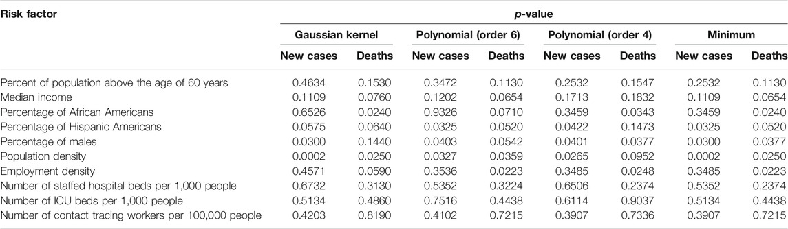
TABLE 1. p-values for testing 10 scalar potential causes of the number of new cases and deaths of COVID-19 in the US.
Population density was an important risk factor for both the spread and death from COVID-19. High density resulted in closer contact, stronger interaction among residents and lower social distancing, which facilitated the spread and increased the death rate from COVID-19 [45–48]. However, our results were contradictory with the conclusion of Hamidi et al. [49]. Some literature also confirmed that high proportion of African Americans caused a high rate of deaths [48, 50, 51]. Our results concluded that percentage of Hispanic Americans was a risk factor for the spread and a weak risk factor for death from COVID-19, while the literature showed stronger evidence that Hispanic communities were highly vulnerable to COVID-19 [52].
The second most significant demographic risk factor for the spread of COVID-19 was percentage of males. We found higher COVID-19 morbidity in males than females. However, we did not find higher COVID-19 mortality in males than females.
It was reported that higher COVID-19 mortality in males than females can be due to the following factors [53]. The first factor was higher expression of angiotensin-converting enzyme-2 (ACE two; receptors for coronavirus) in males than females. The second factor was sex-based immunological differences due to sex hormone and the X chromosome.
Test for Granger Causality
Daily mobility and social distancing data from a COVID-19 impacted the analysis platform, including four categories: category A: mobility and social distancing, category B: COVID and health, category C: economic impact, and category D: vulnerable population. A total of 12 temporal metrics in four categories and 12 metrics from the COVID-19 impact analysis platform, six daily Google Community Mobility indexes and protest attendee data that captured real-time trends in movement patterns for each state in the US were included in the analysis to test for Granger causality between these risk factors, health intervention measures and the number of new cases and deaths from COVID-19 across 50 states in the US [44, 54]. The total number of variables to be tested was 18. The p-value for declaring significance after Bonferroni correction was 0.0028.
All 18 metrics except for protest attendee showed high significance in causing a reduction of the new cases of COVID-19 in 19 less affected states: VT, WY, ME, AK, NH, WV, ND, SD, NM, RI, DE, KY, KS, CT, CO, IA, WA, WI, and MS. Most of these states were less populated. However, although CA was most affected and the most populated state, all 18 metrics except protest attendance showed a strong significance in causing rapid spread of COVID-19 (Table 2 and Supplementary Table S1). To provide complete causal testing information, we listed the values of statistics for testing 18 temporal potential causes of the number of new cases of COVID-19 across 50 states in the US in Supplementary Table S2.
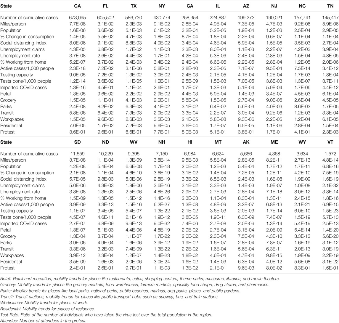
TABLE 2. p-values testing 18 temporal potential causes of the number of new cases of COVID-19 in the top 10 most affected states and bottom 10 less affected states in the US.
All 18 metrics showed no significance in causing reduction of the new cases of COVID-19 in Florida. The majority of the 18 metrics did not demonstrate evidence that they can significantly mitigate the spread of COVID-19 in most the affected states such as TX, NY, GA, IL, AZ, NJ, NC, and TN. These 10 states were in the top largest states by population in the US. Public health intervention measures such as closing schools and businesses, avoiding public gatherings, restricting traffic, placing residents to stay-at-home and adherence to guidelines were less well implemented or difficult to implement homogeneously due to large populations and geographical areas [55]. These results also explained why the number of new cases of COVID-19 in these states was high and confirmed by several studies [56–58].
Table 3 summarized the ranges of p-values, Supplementary Tables S3, S4 summarized all p-values and values of statistics for testing 18 temporal potential causes of the number of new deaths from COVID-19 across 50 states in the US, respectively. All 18 metrics except for protest attendance showed high significant evidence for causing a reduction of new deaths across 50 states except for Michigan (MI) in the US. Our results suggested that a cascade of causes led to the COVID-19 tragedy in the US.
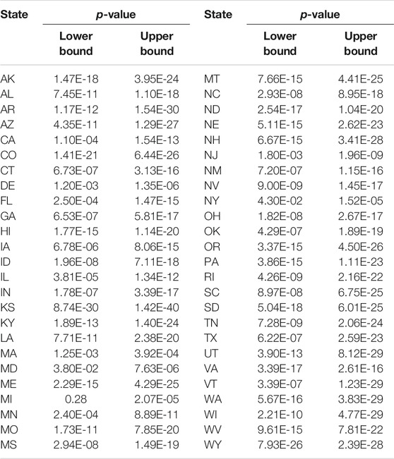
TABLE 3. Ranges of p-values for testing 18 temporal potential causes of the number of new deaths from COVID-19 across 50 states in the US.
Table 4 listed the most significant risk factor for the new cases of COVID-19 in each of the 50 states in the US. Active Cases/1,000 People, workplaces, number of tests completed/1,000 people, imported COVD cases, unemployment rate and unemployment claims/1,000 people, mobility trends for places of residence (residential), retail and recreation, mobility trends for places like restaurants, cafes, shopping centers, theme parks, museums, libraries, and movie theaters (retail) and test capacity were the most significant risk factors for the new cases of COVID-19 in 23, 7, 6, 5, 4, 2, 1 and 1 states of the US, respectively.
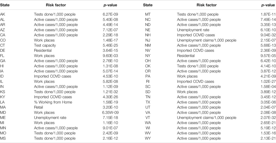
TABLE 4. The most significant risk factor for the new cases of COVID-19 in each of 50 states in the US.
Table 5 summarized the most significant risk factor for the deaths from COVID-19 in each of the 50 states in the US. Active Cases/1,000 people, workplaces, residential, unemployment rate, imported COVID cases, unemployment claims/1,000 people, transit, test done/1,000 people, grocery, testing capacity, retail, percentage of change in consumption, percentage of working from home were the most significant risk factor for the deaths of COVID-19 in 17, 10, 4, 4, 3, 2, 2, 2, 1, 1, 1, 1 states, respectively. We also observed that the number of protest attendees showed mild significant evidence to cause increasing the number of new cases of COVID-19 in KY (p-value < 0.00012), KS (p-value < 0.00026), NH (p-value < 0.00108), MA (p-value < 0.0016) and TN (p-value < 0.0024) or to cause more deaths from COVID-19 in OR (p-value < 5.11 E-05), TX (p-value < 0.00017), ME (p-value < 0.00028), KS (p-value < 0.00061), MI (p-value < 0.0015), OH (p-value < 0.0021) and NC (p-value < 0.0023).
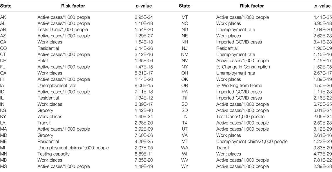
TABLE 5. The most significant risk factor for deaths of COVID-19 in each of 50 states in the US.
In some cases, two causal directions may occur. To examined whether the COVID-19 cases and deaths caused daily mobility and social distancing metrics to change, we summarized the values of statistics and p-values for testing COVID-19 new case and death potential causes of six Google mobility indexes across 50 states in the US in Supplementary Tables S5–7 and DS8, respectively. We did observe the opposite causal direction. Table 6 presented the smallest p-value across 50 states in the US for testing two causal directions: from Google mobility indexes to the number of new cases of COVID-19 and from the number of new cases of COVID-19 to the Google mobility indexes. We observed significant causation from the number of COVID-19to the Google mobility indexes in some states. However, the p-values for testing causation from the number of new cases of COVID-19 to the Google mobility indexes were much larger than that from the Google mobility indexes to the number of new cases of COVID-19. The causal pattern for the COVID-19 deaths was similar to the number of new cases of COVID-19.

TABLE 6. Lower bound of p-values for testing causation from Google mobility indexes to COVID-19 case and from COVID-19 case to Google mobility indexes.
To illustrate the causal relationships between the risk factors and the number of new cases and deaths from COVID-19, we plotted Figures 1 and 2. Figure 1 plotted the social distance index curves as a function of time from March 5, 2020 to August 25, 2020 in Florida (FL) and Rhode Island (RI). Figure 1 showed that the social distance index in FL was much higher than that in RI state, which resulted in the larger number of new cases of COVID-19 in FL than that in RI. Figure 2 showed the number of imported COVID-19 cases as a function of time from March 5, 2020 to August 25, 2020 in Maryland (MD) and Wyoming (WY). We observed a huge difference in the number of imported COVID-19 cases between MD and RI. The very low number of imported cases of COVID-19 in WY resulted in the very low number of deaths from COVID-19 in WY, while the high number of imported cases in MD state led to the increased deaths from COVID-19 in MD. These results were consistent with the finding in the literature. It was reported that strong interventions would substantially decrease the number of deaths (Davies et al. 2020; Gagnon et al. 2020).
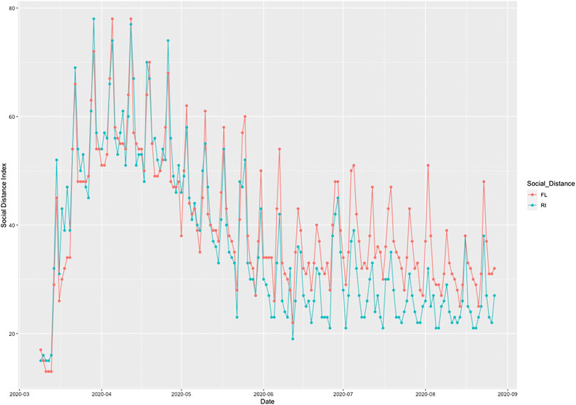
FIGURE 1. Social distance index curves as a function of time from March 5, 2020 to August 25, 2020 in Florida (FL) (red color) and Rhode Island (RI) (blue color).
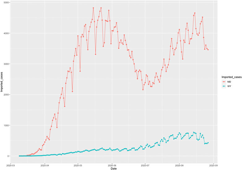
FIGURE 2. Number of imported COVID-19 cases as a function of time from March 5, 2020 to August 25, 2020 in Maryland (MD) (red color) and Wyoming (WY) (blue color).
The COVID-19 case curves as a function of time from March 5, 2020 to August 25, 2020 in FL, RI, MD and WY were plotted in Figure 3, respectively. The response of COVID-19 to public health intervention which were measured by Google mobility indexes were usually delayed.
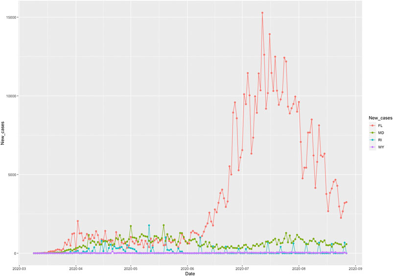
FIGURE 3. Number of new cases of COVID-19 as a function of time from March 5, 2020 to August 25, 2020 in Florida (FL), Rhode Island (RI), Maryland (MD), and Wyoming (WY).
Discussion
Causal inference for COVID-19 is essential for selecting and implementing public intervention measures and understanding the role of the demographics in curbing the spread and reducing the deaths from COVID-19. In this paper, we systematically addressed the issues in identifying causal risk factors and evaluating the causal effects of risk factors and intervention measures on the spread and deaths from COVID-19 in the US. Risk factors and intervention measures included scalar variables and temporal variables. The ANMs were used to test for causal relationships between scalar risk factors and the average number of new cases or deaths from COVID-19 in the US. Transmission of COVID-19 is a dynamic system. Many risk factors and intervention measures are temporal variables. The Granger Causality Test was used to reveal the causal relationships between the temporal risk factors and intervention measures, and the number of new cases or new deaths from COVID-19 across the 50 states in the US.
The demographic risk factors were the major part of the scalar risk factors in the causal analysis of COVID-19. We found that population density was the most significant causal factor of both new cases and death from COVID-19. Population density measured the average number of people per square kilometer living in a built-up area. Densely populated states generated conditions where COVID-19 can spread quickly and undetected in the densely populated areas and created high levels of vulnerability. The second significant demographic factor was percentage of males. Our data suggested that men were more vulnerable to COVID-19 than women. However, our analysis did not conclude that more men than women were dying from COVID-19.
We also discovered that more Black Americans were dying from COVID-19. The reasons for this were complex. Black Americans had higher rates of chronic disease conditions, including diabetes, heart disease, and lung disease, were poor and more easily exposed to the COVID-19, and lived in the cramped housing. Inequities in the social determinants of health affected mortality and morbidity of COVID-19 for Hispanic Americans with much milder significance.
We studied the causal effect of major public health interventions across the 50 states in the US. In the absence of centralized intervention measures and implementation of a timeline and presence of the complex dynamics of human mobility and the variable intensity of local outbreaks of COVID-19, evaluating the causal effect of public health intervention measures on COVID-19 transmission and deaths in the USA posed a great challenge. We used 6 Google mobility indexes and 12 daily metrics to measure the effects of COVID-19 spread and public health interventions on mobility and social distancing, derived from mobile device location data and COVID-19 case data, provided by the University of Maryland COVID-19 Impact Analysis Platform. These real time metrics capture the dynamics of social distancing. Granger causality tests were used to identify the causality relationships between time series metrics and time varying in the number of new cases or deaths from COVID-19. Although the risk factors differed by location, Active Cases/1,000 people were a significant risk factor for both number of new cases and deaths from COVID-19 in most states. The most popular intervention measure in the US was workplaces (mobility trends for places of work). Workplaces were the significant cause of the number new cases of COVID-19 in 44 states and significant cause of death in 49 states. Therefore, workplaces should be considered as a very important risk mitigation measure to reduce the number of new cases and deaths from COVID-19. Tests done/1,000 people was the second population intervention in the US. It was the significant cause of the new cases of COVID-19 in 46 states and significant cause of death in 47 states. Virus test results in quick case identification and isolation to contain COVID-19, and rapid treatment to reduce the number of deaths. Imported COVID cases were also a top significant risk factor for speeding the spread and increasing the deaths from COVID-19. Our results showed that the imported COVID case metric was the significant causal factor for the new cases in 46 states and the significant causal factor for the deaths in 47 states.
Our results showed that the high numbers of cases and deaths from COVID-19 were due to lacking strong interventions and high population density. We observed that no metrics showed significant evidence in mitigating the COVID-19 epidemic in FL and only a few metrics showed evidence in reducing the number of new cases of COVID-19 in AZ, NY and TX. Our results showed strong interventions were needed to contain COVID-19.
Although we tried to systematically and comprehensively analyze the data, this study has multiple limitations. First, we only analyzed the causal relationship between mobility patterns and the number of new cases or deaths and ignored the role of other potential mitigating factors (e.g., wearing face masks) that could also have contributed to the reduction of new cases or deaths from COVID-19. When data are available, more metrics should be included in the analysis.
Second, we have not addressed the confounding bias issue. When confounding is unknown, adjusting for confounding methods cannot be applied to eliminate confounding bias from the causal analysis. Unadjusted confounding bias will distort the inferred (true) causal relationship between the number of new cases or deaths from COVID-19, and metrics for social distancing when these two variables share common causes. This will have substantive implications for developing interventions to mitigate the spread of COVID-19 and reduce the deaths from COVID-19. However, removing confounding from causal analysis for COVID-19 is complicated and will be investigated in the future.
In summary, our analysis has provided information for both individuals and governments to plan future interventions on containing COVID-19 and reduction of deaths from COVID-19.
Data Availablity Statement
The original contributions presented in the study are included in the article/Supplementary Material, further inquiries can be directed to the corresponding author.
Author Contributions
ZL, data analysis; TX, data analysis; KZ, data acquisition and interpretation; H-WD, interpretation; EB, biological interpretation; MX, concept design, method development and write a manuscript.
Funding
H-WD was partially supported by NIH Grants Nos. U19AG05537301 and R01AR069055. MX was partially supported by NIH Grants No. U19AG05537301.
Conflict of Interest
The authors declare that the research was conducted in the absence of any commercial or financial relationships that could be construed as a potential conflict of interest.
Acknowledgments
The authors thank Sara Barton for editing the manuscript. The authors also thank the reviewers for their helpful comments.
Supplementary Material
The Supplementary Material for this article can be found online at: https://www.frontiersin.org/articles/10.3389/fams.2020.611805/full#supplementary-material.
References
1. Callaway, E. Time to use the p-word? Coronavirus enters dangerous new phase. Nature (2020). doi:10.1038/d41586-020-00551-1
2. Priyadarsini, SL, and Suresh, M. Factors influencing the epidemiological characteristics of pandemic COVID 19: a TISM approach. Int J Healthc Manag (2020). 13:89–98. doi:10.1080/20479700.2020.1755804
3. Irfan, U. The math behind why we need social distancing, starting right now. (2020). Available from: https://www.vox.com/2020/3/15/21180342/coronavirus-covid-19-us-social-distancing (Accessed March 15, 2020).
4. Farseev, A, Chu-Farseevac, YY, Yanga, Q, and Loo, DB. Understanding economic and health factors impacting the spread of COVID-19 disease. medRxiv [Preprint] (2020). Available from: https://doi.org/10.1101/2020.04.10.20058222 (Accessed June 9, 2020).
5. Tantrakarnapa, K, Bhopdhornangkul, B, and Nakhaapakorn, K. Influencing factors of COVID-19 spreading: a case study of Thailand. J Public Health (2020). [Epub ahead of print]. doi:10.1007/s10389-020-01329-5
6. Nakada, LYK, and Urban, RC. COVID-19 pandemic: environmental and social factors influencing the spread of SARS-CoV-2 in the expanded metropolitan area of São Paulo, Brazil. Environ Sci Pollut Res Int (2020). 28:1–7. doi:10.1007/s11356-020-10930-w
7. Chaudhry, R, Dranitsaris, G, Mubashir, T, Bartoszko, J, and Riazi, S. A country level analysis measuring the impact of government actions, country preparedness and socioeconomic factors on COVID-19 mortality and related health outcomes. WClinical Medicine (2020). 25:100464. doi:10.1016/j.eclinm.2020.100464
8. Baum, CF, and Henry, M. Socioeconomic factors influencing the spatial spread of COVID-19 in the United States. In: Boston college working papers in economics, 1009. Boston College Department of Economics (2020).
9. Coccia, M. Factors determining the diffusion of COVID-19 and suggested strategy to prevent future accelerated viral infectivity similar to COVID. Sci Total Environ (2020). 729:138474. doi:10.1016/j.scitotenv.2020.138474
10. Livadiotis, G. Statistical analysis of the impact of environmental temperature on the exponential growth rate of cases infected by COVID-19. PloS One (2020). 15(5):e0233875. doi:10.1371/journal.pone.0233875
11. Zhou, F, Yu, T, Du, R, Fan, G, Liu, Y, Liu, Z, et al. Clinical course and risk factors for mortality of adult inpatients with COVID-19 in Wuhan, China: a retrospective cohort study. Lancet (2020). 395:1054–1062. doi:10.1016/S0140-6736(20)30566-3
12. Raghupathi, V. An empirical investigation of chronic diseases: a visualization approach to Medicare in the United States. Int J Healthc Manag (2019). 12(4):327–39. doi:10.1080/20479700.2018.1472849
13. Anderson, RM, Hollingsworth, TD, Baggaley, RF, Maddren, R, and Vegvari, C. COVID-19 spread in the UK: the end of the beginning? Lancet (2020). 396(10251):587–90. doi:10.1016/S0140-6736(20)31689-5
14. Saadat, S, Rawtani, D, and Hussain, CM. Environmental perspective of COVID-19. Sci Total Environ (2020). 728(2020):138870. doi:10.1016/j.scitotenv.2020.138870
15. Flaxman, S, Mishra, S, Gandy, A, Unwin, HJT, Mellan, TA, Coupland, H, et al. Estimating the effects of non-pharmaceutical interventions on COVID-19 in Europe. Nature (2020). 584:257–61. doi:10.1038/s41586-020-2405-7
16. MonodUnwin, RM, Russell, SJ, Croker, H, Packer, J, Ward, J, Stansfield, C, et al. School closure and management practices during coronavirus outbreaks including COVID-19: a rapid systematic review. Lancet Child Adolesc Health (2020). 4:397–404. doi:10.1016/S2352-4642(20)30095-X
17. BooyMytton, J, Miller, BS, Manning, EM, Lampos, V, Zhuang, M, Edelstein, M, et al. Digital technologies in the public-health response to COVID-19. Nat Med (2020). 26:1183–92. doi:10.1038/s41591-020-1011-4
18. McKendryRees, CN, Iboi, E, Eikenberry, S, Scotch, M, MacIntyre, CR, Bonds, MH, et al. Mathematical assessment of the impact of non-pharmaceutical interventions on curtailing the 2019 novel Coronavirus. Math Biosci (2020). 325:108364. doi:10.1016/j.mbs.2020.108364
19. Gumel, SM, and Radovic, A. Digital approaches to remote pediatric health care delivery during the COVID-19 pandemic: existing evidence and a call for further research. JMIR Pediatr Parent (2020). 3(1):e20049. doi:10.2196/20049
20. Altman, N, and Krzywinski, M Association, correlation and causation. Nat Methods (2015). 12(10):899–900. doi:10.1038/nmeth.3587
21. Sharkey, P, and Wood, G. The causal effect of social distancing on the spread of SARS-CoV-2 (2020). Available from: https://doi.org/10.31235/osf.io/hzj7a (Accessed May 19, 2020).
22. Steigera, E, Mußgnuga, T, and Kroll, LE. Causal analysis of COVID-19 observational data in German districts reveals effects of mobility, awareness, and temperature. medRxiv [Preprint] (2020). Available from: https://doi.org/10.1101/2020.07.15.20154476 (Accessed July 23, 2020).
23. Li, AY, Hannah, TC, Durbin, J, Dreher, N, McAuley, FM, Marayati, NF, et al. Multivariate analysis of factors affecting COVID-19 case and death rate in U.S counties: the significant effects of Black race and temperature. Am Med J Sci (2020). 360(4):348–56. doi:10.1016/j.amjms.2020.06.015
24. Zenil, H, Kiani, NA, Zea, AA, and Tegnér, J. Causal deconvolution by algorithmic generative models. Nat Mach Intell (2019). 1:58–66. doi:10.18148/srm/2020.v14i2.7723
25. Ramachandra, V, and Sun, H. Causal inference for COVID-19 interventions. medRxiv [Preprint] (2020). Available from: https://doi.org/10.1101/2020.09.29.20203505 (Accessed September 29, 2020).
26. Friston, KJ, Parr, T, Zeidman, P, Razi, A, Flandin, G, Daunizeau, J, et al. Dynamic causal modelling of COVID-19. Wellcome Open Res (2020). 5:89. doi:10.12688/wellcomeopenres.15881.2
27. LambertHulme, V, Kasahara, H, and Schrimpf, P. Causal impact of masks, policies, behavior on early COVID-19 pandemic in the U.S. medRxiv [Preprint] (2020). Available from: https://doi.org/10.1101/2020.05.27.20115139 (Accessed September 12, 2020).
28. Regis Annea, W, and Carolin Jeeva, S. ARIMA modelling of predicting COVID-19 infections. medRxiv [Preprint] (2020). Available from: https://doi.org/10.1101/2020.04.18.20070631 (Accessed April 23, 2020).
29. Peters, J, Mooij, JM, Janzing, D, and Schölkopf, B. Causal discovery with continuous additive noise models. J Mach Learn Res (2014). 15:2009–53. 10.15496/publikation-1672
30. Johansen, S. Estimation and hypothesis testing of cointegration vectors in Gaussian vector autoregressive models. Econometrica (1991). 59(6):1551–80. doi:10.2307/2938278
31. Granger, CWJ. Investigating causal relations by econometric models and cross-spectral methods. Econometrica (1969). 37:424–38. doi:10.2307/1912791
32. Eichler, M. Causal inference with multiple time series: principles and problems. Philos Trans A Math Phys Eng Sci (2013). 371:20110613. doi:10.1098/rsta.2011.0613
33. Bai, ZD, Wong, WK, and Zhang, BZ. Multivariate linear and nonlinear causality tests. Math Comput Simulat (2010). 81:5–17. doi:10.1371/journal.pone.0185155
34. Jiao, R, Lin, N, Hu, Z, Bennett, DA, Jin, L, and Xiong, M. Bivariate causal discovery and its applications to gene expression and imaging data analysis. Front Genet (2018). 9:347. doi:10.3389/fgene.2018.00347
35. Mooij, JM, Peters, J, Janzing, D, Zscheischler, J, and Schölkopf, B. Distinguishing cause from effect using observational data: methods and benchmarks. J Mach Learn Res (2016). 17(32):1–102.
36. Heydari, MR, Salehkaleybar, S, and Zhang, K. Adversarial orthogonal regression: two non-linear regressions for causal inference (2019). Available at: https://arxiv.org/abs/1909.04454 (Accessed September 10, 2019).
38. Lu, S, Shen, Y, and Wang, Y. Generalized high-precision simulation for TT&C channels using B-spline signal processing. IEEE Signal Process Lett (2017). 24(9):1383–7. doi:10.1109/LSP.2017.2727524
39. Cleveland, WS. Robust locally weighted regression and smoothing scatterplot. J Am Stat Assoc (1979). 74(368):829–36. 10.1080/01621459.1979.10481038
40. Gretton, A, Bousquet, O, Smola, A, and Schölkopf, B. Measuring statistical dependence with Hilbert–Schmidt norms. Proceedings of the International Conference on Algorithmic Learning Theory; 2005 October 8–11; Singapore (2005). 63–77.
41. Vakhania, NN, Tarieladze, VI, and Chobanyan, SA. Covariance operators. In: Probability distributions on banach spaces. Mathematics and its application (soviet series), Vol. 14. Dordrecht: Springer (1987).
42. Abdalla, I, and Murinde, V. Exchange rate and stock price interactions in emerging financial markets: evidence on India, Korea, Pakistan and the Philippines. Appl Financ Econ (1997). 7:25–35. doi:10.1080/096031097333826
43.Maryland Transportation Institute. University of Maryland COVID-19 impact analysis platform. College Park, USA: University of Maryland (2020). Available from: https://data.covid.umd.edu (Accessed 2020).
44. Zhang, L, Ghader, S, Pack, M, Darzi, A, Xiong, C, Yang, M, et al. An interactive COVID-19 mobility impact and social distancing analysis platform. medRxiv [Preprint] (2020). Available from: https://doi.org/10.1101/2020.04.29.20085472 (Accessed May 5, 2020).
45. Rocklöv, J, and Sjödin, H. High population densities catalyse the spread of COVID-19. J Trav Med (2020). 27(3):taaa038. doi:10.1093/jtm/taaa038
46. Pequeno, P, Mendel, B, Rosa, C, Bosholn, M, Souza, JL, Baccaro, F, et al. Air transportation, population density and temperature predict the spread of COVID-19 in Brazil. PeerJ (2020). 8:e9322. doi:10.7717/peerj.9322
47. MagnussonBarbosa, E. High population density in India associated with spread of COVID-19. Medical Research News (2020). Available from: https://www.news-medical.net/news/20200703/High-population-density-in-India-associated-with-spread-of-COVID-19.aspx (Accessed July 3, 2020).
48. Rajan, K, Dhana, K, Barnes, LL, Aggarwal, NT, Evans, L, Wilson, RS, et al. Strong effects of population density and social characteristics on distribution of COVID-19 infections in the United States. medRxiv [Preprint] (2020). Available from: https://doi.org/10.1101/2020.05.08.20073239 (Accessed May 19, 2020).
49. Hamidi, S, Sabouri, S, and Ewing, R. Does density aggravate the COVID-19 pandemic? J Am Plann Assoc (2020). 86:495–509. doi:10.1080/01944363.2020.1777891
50. Golestaneh, L, Neugarten, J, Fisher, M, Billett, HH, Gil, MR, Johns, T, et al. The association of race and COVID-19 mortality. EClinicalMedicine (2020). 25:100455. doi:10.1016/j.eclinm.2020.100455
51. BellinYunes, UV, and Larkins-Pettigrew, M. Racial demographics and COVID-19 confirmed cases and deaths: a correlational analysis of 2886 US counties. J Public Health (2020). 42(3):445–7. doi:10.1093/pubmed/fdaa070
52. Calo, WA, Murray, A, Francis, E, Bermudez, M, and Kraschnewski, J. Reaching the hispanic community about COVID-19 through existing chronic disease prevention programs. Prev Chronic Dis (2020). 17:200165. doi:10.5888/pcd17.200165
53. Bwire, GM. Coronavirus: why men are more vulnerable to covid-19 than women?. SN Compr Clin Med (2020). 4:1–3. doi:10.1007/s42399-020-00341-w
54.Google community mobility reports. (2020). Available from: https://www.google.com/covid19/mobility/ (Accessed August 17, 2020).
55. Althouse, BM, Wallace, B, Case, B, Scarpino, SV, Berdhal, A, White, ER, et al. The unintended consequences of inconsistent pandemic control policies. medRxiv [Preprint] (2020). Available from: https://doi.org/10.1101/2020.08.21.20179473 (Accessed October 28, 2020).
56. Hebert-Dufresne, S, Ruktanonchai, NW, Zhou, L, Prosper, O, Luo, W, Floyd, JR, et al. Effect of non-pharmaceutical interventions to contain COVID-19 in China. medRxiv [Preprint] (2020). Available from: https://doi.org/10.1101/2020.03.03.20029843 (Accessed March 13, 2020).
57. Masrur, A, Yu, M, Luo, W, and Dewan, A. Space-time patterns, change, and propagation of COVID-19 risk relative to the intervention scenarios in Bangladesh. Int J Environ Res Publ Health (2020). 17(16):E5911. doi:10.3390/ijerph17165911
Keywords: COVID-19, causal inference, time series, control of the spread, transmission dynamics, public health interventions
Citation: Li Z, Xu T, Zhang K, Deng H-W, Boerwinkle E and Xiong M (2021) Causal Analysis of Health Interventions and Environments for Influencing the Spread of COVID-19 in the United States of America. Front. Appl. Math. Stat. 6:611805. doi: 10.3389/fams.2020.611805
Received: 29 September 2020; Accepted: 03 December 2020;
Published: 25 January 2021.
Edited by:
Zhanwei Du, University of Texas at Austin, United StatesCopyright © 2021 Li, Xu, Zhang, Deng, Boerwinkle and Xiong. This is an open-access article distributed under the terms of the Creative Commons Attribution License (CC BY). The use, distribution or reproduction in other forums is permitted, provided the original author(s) and the copyright owner(s) are credited and that the original publication in this journal is cited, in accordance with accepted academic practice. No use, distribution or reproduction is permitted which does not comply with these terms.
*Correspondence: Momiao Xiong, TW9taWFvLlhpb25nQHV0aC50bWMuZWR1