 Guohua Gao
 Horacio Florez1
- 1Shell Global Solutions (United States) Inc., Houston, TX, United States
- 2Shell Global Solutions International B.V., Amsterdam, Netherlands
The limited-memory Broyden–Fletcher–Goldfarb–Shanno (L-BFGS) optimization method performs very efficiently for large-scale problems. A trust region search method generally performs more efficiently and robustly than a line search method, especially when the gradient of the objective function cannot be accurately evaluated. The computational cost of an L-BFGS trust region subproblem (TRS) solver depend mainly on the number of unknown variables (n) and the number of variable shift vectors and gradient change vectors (m) used for Hessian updating, with m << n for large-scale problems. In this paper, we analyze the performances of different methods to solve the L-BFGS TRS. The first method is the direct method using the Newton-Raphson (DNR) method and Cholesky factorization of a dense n × n matrix, the second one is the direct method based on an inverse quadratic (DIQ) interpolation, and the third one is a new method that combines the matrix inversion lemma (MIL) with an approach to update associated matrices and vectors. The MIL approach is applied to reduce the dimension of the original problem with n variables to a new problem with m variables. Instead of directly using expensive matrix-matrix and matrix-vector multiplications to solve the L-BFGS TRS, a more efficient approach is employed to update matrices and vectors iteratively. The L-BFGS TRS solver using the MIL method performs more efficiently than using the DNR method or DIQ method. Testing on a representative suite of problems indicates that the new method can converge to optimal solutions comparable to those obtained using the DNR or DIQ method. Its computational cost represents only a modest overhead over the well-known L-BFGS line-search method but delivers improved stability in the presence of inaccurate gradients. When compared to the solver using the DNR or DIQ method, the new TRS solver can reduce computational cost by a factor proportional to
Introduction
Decision-making tools based on optimization procedures have been successfully applied to solve practical problems in a wide range of areas. An optimization problem is generally defined as minimizing (or maximizing) an objective function
In the oil and gas industry, an optimal business development plan requires robust production optimization because of the considerable uncertainty of subsurface reservoir properties and volatile oil prices. Many papers have been published on the topic of robust optimization and their applications to cyclic CO2 flooding through the Gas-Assisted Gravity Drainage process [1], well placement optimization in geologically complex reservoirs [2], optimal production schedules of smart wells for water flooding [3] and in naturally fractured reservoirs [4], just mentioning a few of them as examples.
Some researchers formulated the optimization problem under uncertainty as a single objective optimization problem, e.g., only maximizing the mean of net present value (NPV) for simplicity by neglecting the associated risk. However, it is recommended to formulate robust optimization as a bi-objective optimization problem for consistency and completeness. A bi-objective optimization problem is generally defined as minimizing (or maximizing) two different objective functions,
It is also a very challenging task to properly characterize the uncertainty of reservoir properties (e.g., porosity and permeability in each grid-block) and reliably quantify the ensuing uncertainty of production forecasts (e.g., production rates of oil, gas, and water phases) by conditioning to historical production data and 4D seismic data [7, 8], which requires generating multiple conditional realizations by minimizing a properly defined objective function, e.g., using the randomized maximum likelihood (RML) method [9].
When an adjoint-based gradient of the objective function is available [10–12], we may apply a gradient-based optimization method, e.g., the Broyden–Fletcher–Goldfarb–Shanno (BFGS) optimization method [13, 14]. However, the adjoint-based gradient is not available for many commercial simulators and not available for integer type or discrete variables (e.g., well locations defined by grid-block indices). In such a case, we must apply a derivative-free optimization (DFO) method [15–18]. For problems with smooth objective functions and continuous variables, model-based DFO methods using either radial-basis function [19] or quadratic model [16, 20, 21] performs more efficiently than other DFO methods such as direct pattern search methods [22] and stochastic search methods [23].
Traditional optimization methods only locate a single optimal solution, and they are referred to as single-thread optimization methods in this paper. It is unacceptably expensive to use a single-thread optimization method to locate multiple optimal solutions on the Pareto front or generate multiple RML samples [24]. To overcome the limitations of single-thread optimization methods, Gao et al. [17] developed a local-search distributed Gauss-Newton (DGN) DFO method to find multiple best matches concurrently. Later, Chen et al. [25] modified the local-search DGN optimization method and generalized the DGN optimizer for global search. They also integrated the global-search DGN optimization method with the RML method to generate multiple RML samples in parallel.
Because multiple search points are generated in each iteration, finally, multiple optimal solutions can be found in parallel. These distributed optimization methods are referred to as multiple-thread optimization methods. Both the local- and global-search DGN optimization methods are only applicable to a specific optimization problem, i.e., history matching problem or least-squares optimization problem, of which the objective function can be expressed as a form of least-squares,
Recently, Gao et al. [18] developed a well-paralleled distributed quasi-Newton (DQN) DFO method for generic optimization problems by introducing a generalized form of the objective function,
In Eq. 1,
The DQN optimization algorithm runs Ne optimization threads in parallel. In the k-th iteration, there are
All simulation results generated by all DQN optimization threads in previous and current iterations are recorded in a training data set, and they are shared among all DQN optimization threads. The sensitivity matrix
Both DGN and DQN optimization methods approximate the objective function by a quadratic model, and they are designed for problems with smooth objective function and continuous variables. Although their convergence is not guaranteed for problems with integer type variables (e.g., well location optimization), if those integers can be treated as truncated continuous variables, our numerical tests indicate that these distributed optimization methods can improve the objective function significantly and locate multiple suboptimal solutions for problems with integer type variables in only a few iterations.
The number of variables for real-world problems may vary from a few to thousands or even more, depending on the problem and the parameterization techniques employed. For example, the number of variables could be in the order of millions if we do not apply any parameter reduction techniques to reduce the dimension of some history matching problems (e.g., to tune permeability and porosity in each grid block). Because reservoir properties are generally correlated with each other with long correlation lengths, we may reduce the number of variables to be tuned to only a few hundred, e.g., using the principal component analysis (PCA) or other parameter reduction techniques [26].
In this paper, our focus is on performance analysis of different methods to solve the TRS formulated with the limited-memory BFGS (L-BFGS) Hessian updating method for unconstrained optimization problems. In the future, we will further integrate the new TRS solver with our newly proposed limited-memory distributed BFGS (L-DBFGS) optimization algorithm and then apply the new optimizer to some realistic oil/gas field optimization cases and benchmark its overall performance against other distributed optimization methods such as those only using the gradient [27]. We will also continue our investigation in the future for constrained optimization problems (e.g., variables with lower- and/or upper-bounds and problems with nonlinear constraints). Gao et al. [18] applied the popular Newton-Raphson method [28] to directly solve the TRS using matrix factorization, the DNR method in short. The DNR method is quite expensive when it is applied to solve
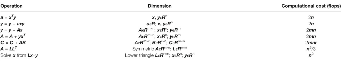
TABLE 1. A summary of computational costs of commonly used algebraic operations.
For completeness, we discuss the compact representation of the L-BFGS Hessian updating formulation [31] and the algorithm to directly update the Hessian in the next section directly. In the third section, we present three different methods to solve the L-BFGS TRS: the DNR method, the direct method using inverse quadratic (DIQ) interpolation approach proposed by Gao et al. [32], and the technique using matrix inversion lemma (MIL) together with an efficient matrix updating algorithm. Some numerical tests and performance comparisons are discussed in the fourth section. We finally draw some conclusions in the last section.
The Limited-Memory Hessian Updating Formulation
Let x(k) be the best solution obtained in the current (k-th) iteration, and f(k), g(k), and H(k), respectively, the objective function, its gradient and Hessian evaluated at x(k). The Hessian H(k+1) is updated using the BFGS formulation as follows,
In Eq. 2,
Compact Representation
To save memory usage and computational cost, the L-BFGS Hessian updating method limits the maximum history size or the maximum number of pairs (s(k), z(k)) used for the BFGS Hessian updating to LM > 1. The recommended value of LM ranges from 5 to 20, using smaller number for problems with more variables.
Let 1 ≤ lk ≤ LM denote the number of pairs of variable shift vectors and gradient change vectors, (s(j), z(j)) for j = 1,2,...lk, used to update the Hessian using the L-BFGS method in the k-th iteration. Let
The Hessian can be updated using the compact form of the L-BFGS Hessian updating formulation [31, 33–35] as follows,
In Eq. 4, In is an n × n identity matrix and W(k) is an m×m symmetric matrix defined as,
In Eq. 4 and Eq. 5,
The Algorithm to Directly Update the Hessian Using the L-BFGS Compact Representation
Given LM ≥ 1, k ≥ 1, lk−1 ≥ 1, the thresholds c3 > 0 and acr > 0, search step
Algorithm-1: Updating the Hessian directly using the L-BFGS compact representation
1. Compute ||s||, ||z||,
2. If
3. Otherwise,
a. Set
b. Update
4. Form
5. Compute
6. Form the matrix
7. Compute
8. Compute
9. Compute
10. Update
11. Stop.
The computational cost to directly update the Hessian using the L-BFGS method as described in Algorithm-1 mainly depends on the number of variables (n) and the number of vectors used to update the Hessian (m = 2lk). We should reemphasize that m is updated iteratively but limited to m ≤ 2Lk. The computational cost is
Solving the L-BFGS Trust Region Subproblem
The Trust Region Subproblem
In the neighborhood of the best solution x(k), the objective function f(x) can be approximated by a quadratic function of
If the Hessian
When a line search strategy is applied, we accept the full search step
The trust region search step
If the solution
For the trivial case with
We may apply the popular DNR method to solve the TRS when
Solving the L-BFGS TRS Directly Using the Newton-Raphson Method
The DNR method solves the TRS defined in Eq. 8 using the Cholesky decomposition. It applies the Newton-Raphson method to directly solve the nonlinear TRS equation [28],
Given the trust region size
Algorithm-2: Solving the L-BFGS TRS Using the DNR Method
1. Initialize
2. Compute
3. Solve
4. Compute
5. If
6. Set
7. Repeat steps (a) through (f) below, until convergence (
a. Update
b. Compute
c. Solve
d. Compute
e. Update
f. Set
8. Stop.
Let
The total computational cost (flops) used to solve the L-BFGS TRS using the DNR method (Algorithm-2) together with the L-BFGS Hessian updating method (Algorithm-1) is,
Our numerical results indicate that the DNR TRS solver may fail when tested on the well-known Rosenbrock function, especially for problems with large
The Inverse Quadratic Model Interpolation Method to Directly Solve the L-BFGS TRS
Instead of applying the Newton-Raphson method which requires evaluating
Both coefficients of
In the first iteration, we set
Let
We either update
Given the scaling factor
Algorithm-3: Solving the L-BFGS TRS Using the DIQ Method
(1) Compute
(2) Calculate
(3) Initialize
(4) Compute
(5) Solve
(6) Compute
(7) If
(8) If
a. Compute
b. Solve
c. Compute
(9) If
(10) Otherwise,
(11) Repeat steps (a) through (i) below, until convergence (
a. Calculate
b. Calculate
c. Compute
d. Solve
e. Compute
f. Update
g. If
h. Otherwise, update
i.
(12) Stop.
Let
Generally, the DIQ method converges faster than the DNR method and it performs more efficiently and robustly than the DNR method, especially for large scale problems. Both the DNR method and the DIQ method become quite expensive for large-scale problems.
Using Matrix Inversion Lemma (MIL) to Solve the L-BFGS TRS
To save both memory usage and computational cost, Gao, et al. [32, 36, 37] proposed an efficient algorithm to solve the Gauss-Newton TRS (GNTRS) for large-scale history matching problems using the matrix inversion lemma (or the Woodbury matrix identity). With appropriate normalization of both parameters and residuals, the Hessian of the objective function for a history matching problem can be approximated by the well-known Gauss-Newton equation as follows,
In Eq. 15,
The GNTRS solver proposed by Gao, et al. [32, 36, 37] using the matrix inversion lemma (MIL) has been implemented and integrated with the distributed Gauss-Newton (DGN) optimizer. Because the compact representation of the L-BFGS Hessian updating formula Eq. 4 is similar to Eq. 15, we follow the similar idea as proposed by Gao, et al. [32, 36, 37] to compute
Let
Then, we compute the trust region search step
From Eq. 15, we have
We first try
Let
In Eq. 21,
Because
Given the
Directly computing the three
Updating Matrices and Vectors Used for Solving the L-BFGS TRS
We first initialize
If
The L-BFGS Hessian updating formulation of Eq. 4 requires
Case-1: Sflag(k) = “False”
Although the best solution
Let
We set
It is straightforward to derive the following equations to update
By definition,
Thus, we have,
Case-2: Sflag(k) = “True” and lk−1 < LM
We set
It is straightforward to derive the following equations to update A(k), B(k), and C(k),
We first split the
where
Because
Case-3: Sflag(k) = “True” and lk−1 = LM
We set
The Algorithm to Update Matrices and Vectors Used for Solving the L-BFGS TRS
Given LM ≥ 1, k > 1, lk−1 ≥ 1, the thresholds c3 > 0 and acr > 0,
Algorithm-4: Updating Matrices and Vectors Used for Solving the L-BFGS TRS
1. Compute
2. Compute the scaling factor
3. If
a. Set
b. Update
c. Update
d. Update
e. Compute
f. Goto step 10.
4. Else if
a. Set
b. Update
c. Set
d. Set
e. Update
f. Compute
g. Compute
h. Compute
i. Update
j. Set
k. Set
l. Update
5. Else if
a. Set
b. Compute
c. Compute
d. Update
e. Set
f. Update
6. Else (for Case-3)
a. Set
b. Remove the first column from
c. Remove the first row and first column from
d. Compute
e. Compute
f. Update
g. Set
h. Set
i. Update
7. Form the matrix
8. Decompose
9. Form the matrix
10. End
The computational cost to update matrices and vectors used for solving the L-BFGS TRS as described in Algorithm-4 is at most
In this paper, we apply the same idea of reducing the dimension from
The Algorithm to Solve the L-BFGS TRS Using the Matrix Inversion Lemma
Given the trust region size
Algorithm-5: Solving the L-BFGS TRS Using the Matrix Inversion Lemma
1. Compute
2. Initialize
3. If
a. Set
b. Set
c. Goto step 11.
4. Compute
5. Solve
6. Compute
7. If
8. Set
9. Repeat steps (a) through (j) below, until convergence (
a. Compute
b. Solve
c. Compute
d. Compute
e. Update
f. Set
g. Compute
h. Solve
i. Compute
j. Set
10. Compute
11. End
Let
The total computational cost (flops) used to solve the L-BFGS TRS using Algorithm-5 together with Algorithm-4 is,
It is straightforward to compute the normalized computational cost, or the ratio of computational cost of the DNR method (Algorithm-2) or the DIQ method (Algorithm-3) together with the algorithm that directly updates Hessian (Algorithm-1) over the MIL TRS solver using the matrix inversion lemma (Algorithm-5) and the efficient matrix updating algorithm (Algorithm-4),
Because
For some problems the solution
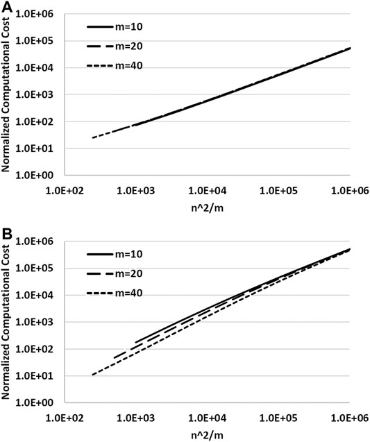
FIGURE 1. Plots of the ratio of computational cost β vs. n2/m, computed using Eq. 35 by fixing
Numerical Validation
We benchmarked the MIL TRS solver against the DNR (or DIQ) TRS solver on two well-known analytic optimization problems using analytical gradients: the Rosenbrock function and the Sphere function defined as follows,
The Rosenbrock function defined in Eq. 37 has one local minimum located at
We implemented different algorithms described in this paper in our in-house C++ optimization library (OptLib). We employ “Armadillo” as our foundational template-based C++ library for linear algebra (http://arma.sourceforge.net/). We ran all test cases reported on Tables 2–5 on a virtual machine computer equipped with an Intel Xeon Platinum Processor at 2.60 MHz and 16.0 GB of RAM. We varied the number of parameters,

TABLE 2. Performance comparison of DNR vs. MIL methods testing on Rosenbrock function.
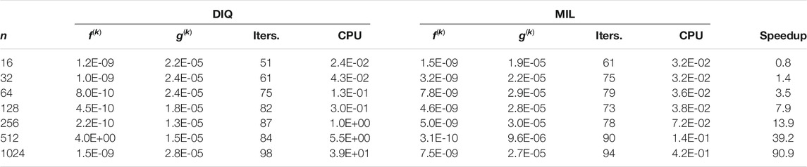
TABLE 3. Performance comparison of DIQ vs. MIL methods testing on Rosenbrock function.
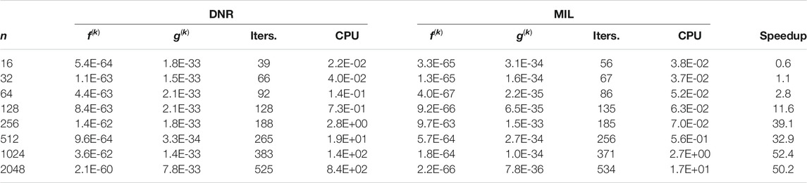
TABLE 4. Performance comparison of DNR vs. MIL methods testing on Sphere function.
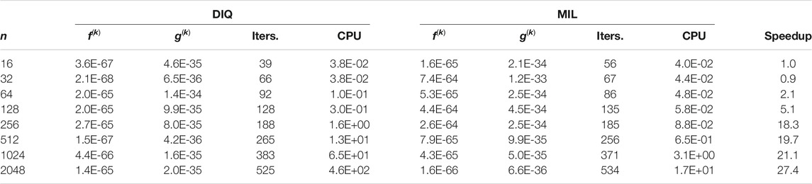
TABLE 5. Performance comparison of DIQ vs. MIL methods testing on Sphere function.
We noticed that the matrix
Table 2 compares performance of the DNR method vs. the MIL methods for the Rosenbrock problem encompassing 8, 16, 32, and 48 parameters, respectively. Beyond those problem sizes, the DNR method could not converge to the solution. Indeed, the DNR method becomes relatively slow, i.e., renders very large lambda values that imply tiny shifts. Often, after 2,048 iterations, the objective function is still greater than one. It seems that the DNR method is not robust enough to tackle the Rosenbrock function with more than 48 parameters. It appears that the MIL method slightly outperforms the DNR method for problems with fewer parameters.
Table 3 compares performance of the DIQ method vs. the MIL method. These numerical results confirm that the MIL method outperforms the DIQ method. As expected, the speedup improves with the increase of the problem size n.
Table 4 shows similar results for the Sphere function problem. We could benchmark the DNR method against the MIL method with ranks up to 2,048 parameters. Again, the speedup increases with problem size. Finally, Table 5 benchmarks the DIQ method against the MIL method testing on the Sphere function. The speedup reduces when compared to Table 4 for the same ranks, but we still clearly see that the performance of the MIL solver exceeds its DIQ counterpart. Results shown in Table 4 and Table 5 also confirm that the DIQ method performs better than the DNR method. We believe that the DIQ TRS solver converges faster with smaller number of iterations than the DNR TRS solver (i.e.,
The computational costs (in terms of CPU time) summarized in Tables 2–5 are the overall costs for all iterations, including the cost of computing both value and gradient of the objective function in addition to the cost of solving the L-BFGS TRS. In contrast, the theoretical analysis results of computational cost for β in Eq. 35 only count for the cost of solving the L-BFGS TRS in just one iteration. Therefore, numerical results listed in Tables 2–5 are not quantitatively in agreement with the theoretically derived β.
Conclusion
We can draw the following conclusions based on theoretical analysis and numerical tests:
1) Using the compact representation of the L-BFGS formulation in Eq. 4, the updated Hessian
2) Using the matrix inversion lemma, we are able to reduce the cost of solving the L-BFGS TRS by transforming the original equation with
3) Further reduction in computational cost is achieved by updating the vector u(k) and matrices such as S(k) and Z(k), A(k), B(k), and C(k), P(k), and
4) Through seamless integration of matrix inversion lemma with the iterative matrix and vector updating approach, the newly proposed TRS solver for the limited-memory distributed BFGS optimization method performs much more efficiently than the DNR TRS solver.
5) The MIL TRS solver can obtain the right solution with acceptable accuracy, without increasing memory usage but reducing the computational cost significantly, as confirmed by numerical results on the Rosenbrock function and Sphere function.
Data Availability Statement
The original contributions presented in the study are included in the article/Supplementary Material, further inquiries can be directed to the corresponding author.
Author Contributions
GG, HF, and JV contributed to conception and algorithmic analysis of the study. HF, TW, FS, and CB contributed to design and numerical validations. GG and FH wrote the first draft of the article. All authors contributed to article revision, read, and approved the submitted version.
Conflict of Interest
Authors GG, HF, and FS were employed by Shell Global Solutions (United States) Inc. Authors JV, TW and CB were employed by Shell Global Solutions International B.V.
References
1. Ai-Mudhafar, WJ, Rao, DN, and Srinivasan, S. Robust Optimization of Cyclic CO2 Flooding through the Gas-Assisted Gravity Drainage Process under Geological Uncertainties. J Pet Sci Eng (2018). 166:490–509. doi:10.1016/j.petrol.2018.03.044
2. Alpak, FO, Jin, L, and Ramirez, BA. Robust Optimization of Well Placement in Geologically Complex Reservoirs. in: Paper SPE-175106-MS Presented at the SPE Annual Technical Conference and Exhibition; September28–30 2015; Houston, TX (2015).
3. van Essen, GM, Zandvliet, MJ, Den Hof, PMJ, Bosgra, OH, Jansen, JD, et al. Robust Optimization of Oil Reservoir Flooding. in: Paper Presented at the IEEE International Conference on Control Applications; Oct 4-6 2006; Munich, Germany (2006). p. 4–6.
4. Liu, Z, and Forouzanfar, F. Ensemble Clustering for Efficient Robust Optimization of Naturally Fractured Reservoirs. Comput Geosci (2018). 22:283–96. doi:10.1007/s10596-017-9689-1
5. Liu, X, and Reynolds, AC. Augmented Lagrangian Method for Maximizing Expectation and Minimizing Risk for Optimal Well-Control Problems with Nonlinear Constraints. SPE J (2016). 21(5). doi:10.1007/s10596-017-9689-1
6. Liu, X, and Reynolds, AC. Gradient-based Multi-Objective Optimization with Applications to Waterflooding Optimization. Comput Geosci (2016). 20:677–93. doi:10.1007/s10596-015-9523-6
7. Oliver, DS, Reynolds, AC, and Liu, N. Inverse Theory for Petroleum Reservoir Characterization and History Matching. Cambridge, United Kingdom: Cambridge University Press (2008). doi:10.1017/cbo9780511535642
8. Tarantola, A. Inverse Problem Theory and Methods for Model Parameter Estimation. Philadelphia, PA: SIAM (2005). doi:10.1137/1.9780898717921
9. Oliver, DS. On Conditional Simulation to Inaccurate Data. Math Geol (1996). 28:811–7. doi:10.1007/bf02066348
10. Jansen, JD. Adjoint-based Optimization of Multi-phase Flow through Porous Media - A Review. Comput Fluids (2011). 46(1):40–51. doi:10.1016/j.compfluid.2010.09.039
11. Li, R, Reynolds, AC, and Oliver, DS. History Matching of Three-phase Flow Production Data. SPE J (2003). 8(4):328–40. doi:10.2118/87336-pa
12. Sarma, P, Durlofsky, L, and Aziz, K. Implementation of Adjoint Solution for Optimal Control of Smart Wells. in: Paper SPE 92864 Presented at the SPE Reservoir Simulation Symposium Held in the Woodlands; Jan.-2 Feb; Woodlands, TX (2005). p. 31.
13. Gao, G, and Reynolds, AC. An Improved Implementation of the LBFGS Algorithm for Automatic History Matching. SPE J (2006). 11(1):5–17. doi:10.2118/90058-pa
15. Chen, C, et al. Assisted History Matching Using Three Derivative-free Optimization Algorithms. in: Paper SPE-154112-MS Presented at the SPE Europec/EAGE Annual Conference Held in Copenhagen; June 4–7 2012; Copenhagen, Denmark (2012). p. 4–7.
16. Gao, G, Vink, JC, Chen, C, Alpak, FO, and Du, K. A Parallelized and Hybrid Data-Integration Algorithm for History Matching of Geologically Complex Reservoirs. SPE J (2016). 21(6):2155–74. doi:10.2118/175039-pa
17. Gao, G, Vink, JC, Chen, C, El Khamra, Y, Tarrahi, M, et al. Distributed Gauss-Newton Optimization Method for History Matching Problems with Multiple Best Matches. Comput Geosciences (2017). 21(5-6):1325–42. doi:10.1007/s10596-017-9657-9
18. Gao, G, Wang, Y, Vink, J, Wells, T, Saaf, F, et al. Distributed Quasi-Newton Derivative-free Optimization Method for Optimization Problems with Multiple Local Optima. in: 17th European Conference on the Mathematics of Oil Recovery ECMOR XVII; September 2020; Edinburgh, United Kingdom (2020). p. 14–7.
19. Wild, SM. Derivative Free Optimization Algorithms for Computationally Expensive Functions. [PhD thesis]. Ithaca (new york): Cornell University (2009).
20. Powell, MJD. Least Frobenius Norm Updating of Quadratic Models that Satisfy Interpolation Conditions. Math Programming (2004). 100(1):183–215. doi:10.1007/s10107-003-0490-7
21. Zhao, H, Li, G, Reynolds, AC, and Yao, J. Large-scale History Matching with Quadratic Interpolation Models. Comput Geosci (2012). 17:117–38. doi:10.1007/s10596-012-9320-4
22. Audet, C, and Dennis, JE Mesh Adaptive Direct Search Algorithms for Constrained Optimization. SIAM J Optim (2006). 17:188–217. doi:10.1137/040603371
23. Spall, JC. Introduction to Stochastic Search and Optimization. Hoboken, NJ: John Wiley & Sons (2003). doi:10.1002/0471722138
24. Chen, C, et al. EUR Assessment of Unconventional Assets Using Parallelized History Matching Workflow Together with RML Method. In: Paper Presented the 2016 Unconventional Resources Technology Conference; August 1–3 2016; San Antonio, TX(2016).
25. Chen, C, Gao, G, Li, R, Cao, R, Chen, T, Vink, JC, et al. Global-Search Distributed-Gauss-Newton Optimization Method and its Integration with the Randomized-Maximum-Likelihood Method for Uncertainty Quantification of Reservoir Performance. SPE J (2018). 23(05):1496–517. doi:10.2118/182639-pa
26. Chen, C, Gao, G, Ramirez, BA, Vink, JC, and Girardi, AM. Assisted History Matching of Channelized Models by Use of Pluri-Principal-Component Analysis. SPE J (2016). 21(05):1793–812. doi:10.2118/173192-pa
27. Armacki, A, Jakovetic, D, Krejic, N, Krklec Jerinkic, N, et al. Distributed Trust-Region Method with First Order Models. in Paper Presented at the IEEE EUROCON-2019, 18th International Conference on Smart Technologies July 1–14 2019 Novi Sad, Serbia (2019). p. 1–4.
28. Moré, JJ, and Sorensen, DC. Computing a Trust Region Step. SIAM J Sci Stat Comput (1983). 4(3):553–72. doi:10.1137/0904038
29. Mohamed, AW. Solving Large-Scale Global Optimization Problems Using Enhanced Adaptive Differential Evolution Algorithm. Complex Intell Syst (2017). 3:205–31. doi:10.1007/s40747-017-0041-0
30. Golub, GH, and Van Loan, CF. Matrix Computations. 4th ed. The Johns Hopkins University Press (2013).
31. Brust, JJ, Leyffer, S, and Petra, CG. Compact Representations of BFGS Matrices. Preprint ANL/MCS-P9279-0120. Lemont, IL: ARGONNE NATIONAL LABORATORY (2020).
32. Gao, G, Jiang, H, Vink, JC, van Hagen, PPH, Wells, TJ, et al. Performance Enhancement of Gauss-Newton Trust-Region Solver for Distributed Gauss-Newton Optimization Method. Comput Geosci (2020). 24(2):837–52. doi:10.1007/s10596-019-09830-x
33. Burdakov, O, Gong, L, Zikrin, S, and Yuan, Y. On Efficiently Combining Limited-Memory and Trust-Region Techniques. Math Prog Comp (2017). 9:101–34. doi:10.1007/s12532-016-0109-7
34. Burke, JV, Wiegmann, A, and Xu, L. Limited Memory BFGS Updating in a Trust-Region framework Tech. Rep. Seattle, WA: University of Washington (2008).
35. Byrd, RH, Nocedal, J, and Schnabel, RB. Representations of Quasi-Newton Matrices and Their Use in Limited Memory Methods. Math Programming (1994). 63:129–56. doi:10.1007/bf01582063
36. Gao, G, Jiang, H, van Hagen, P, Vink, JC, and Wells, T. A Gauss-Newton Trust Region Solver for Large Scale History Matching Problems. SPE J (2017b). 22(6):1999–2011. doi:10.2118/182602-pa
Keywords: limited-memory BFGS method, trust region search optimization method, trust region subproblem, matrix inversion lemma, low rank matrix update
Citation: Gao G, Florez H, Vink JC, Wells TJ, Saaf F and Blom CPA (2021) Performance Analysis of Trust Region Subproblem Solvers for Limited-Memory Distributed BFGS Optimization Method. Front. Appl. Math. Stat. 7:673412. doi: 10.3389/fams.2021.673412
Received: 27 February 2021; Accepted: 29 April 2021;
Published: 24 May 2021.
Edited by:
Olwijn Leeuwenburgh, Netherlands Organisation for Applied Scientific Research, NetherlandsReviewed by:
Andreas Størksen Stordal, Norwegian Research Institute (NORCE), NorwaySarfraz Ahmad, COMSATS University Islamabad, Pakistan
Copyright © 2021 Gao, Florez, Vink, Wells, Saaf and Blom. This is an open-access article distributed under the terms of the Creative Commons Attribution License (CC BY). The use, distribution or reproduction in other forums is permitted, provided the original author(s) and the copyright owner(s) are credited and that the original publication in this journal is cited, in accordance with accepted academic practice. No use, distribution or reproduction is permitted which does not comply with these terms.
*Correspondence: Guohua Gao, Z3VvaHVhLmdhb0BzaGVsbC5jb20=