Three little arbitrage theorems

The authors proved three theorems about the exact solutions of a generalized or interacting Black–Scholes equation that explicitly includes arbitrage bubbles. These arbitrage bubbles can be characterized by an arbitrage number A_N. The first theorem states that if A_N = 0, then the solution at maturity of the interacting equation is identical to the solution of the free Black–Scholes equation with the same initial interest rate of r. The second theorem states that if A_N ≠ 0, then the interacting solution can be expressed in terms of all higher derivatives of the solutions to the free Black–Scholes equation with an initial interest rate of r. The third theorem states that for a given arbitrage number, the interacting solution is a solution to the free Black–Scholes equation but with a variable interest rate of r(τ) = r + (1/τ)A_N(τ), where τ = T − t.

1. Introduction

Since its introduction in 1973, the initial Black–Scholes model [1, 2] has undergone many changes, which have given rise to many different financial models, such as stochastic volatility models [3, 4] and the associated concept of the volatility smile [5, 6] and stochastic rate models [5, 7, 8], which account for the dynamics of the spot interest rate in the determination of option pricing, as well as, for example, the incorporation of jumps; this gives rise to integro differential equations for the price of the option [9]. All these generalizations are related to relaxing some of the assumptions of the initial Black–Scholes (BS) model.

One of the most important of these initial axioms is the non-arbitrage hypothesis, which is associated with equilibrium market dynamics. In analytic terms, the non-arbitrage hypothesis in the BS model can be characterized as follows: if B(t) and S(t) are the risk-free asset and underlying stock prices, the price dynamics of the bond and the stock in the usual BS model are given by the following equations:

$\begin{array}{ll}dB(t)=rB(t)dt,& (1)\end{array}$

$\begin{array}{ll}dS(t)=\alpha S(t)dt+\sigma S(t)dW(t),& (2)\end{array}$

where r is the constant risk-free interest rate, α and σ are the drift rate and the volatility of S, respectively, and W(t) is a Wiener process. To price the financial derivative π, it is assumed that it can be traded, so we can form a portfolio P based on the derivative π and the underlying stock S (no bonds are included). Considering only non-dividend-paying underlying assets and not considering consumption portfolios, the purchase of a new portfolio must be financed only by selling from the current portfolio.

Consider $\overrightarrow{h}(t)=(h_S,h_{\pi })$, where h_S is the number of underlying assets S and h_π is the number of derivatives π present in the portfolio. $\overrightarrow{Z}(t)=(S,\pi )$ is the price vector of shares (underlying asset and option), and the value of the portfolio P at time t is given in equation (3),

$\begin{array}{ll}P(t)=\overrightarrow{h}(t)\overrightarrow{Z}(t)=h_S(t)S(t)+h_{\pi }(t)\pi (S(t),t),& (3)\end{array}$

and the dynamics of a self-financing portfolio with no consumption imply that [5, 7].

$\begin{array}{ll}dP(t)=\overrightarrow{h}(t)d\overrightarrow{Z}(t)=h(t)dS(t)+h_{\pi }(t)d\pi (t).& (4)\end{array}$

In other words, in a model without exogenous incomes or withdrawals, any change in value is due to changes in asset and derivative prices. Another important assumption for deriving the BS equation is that the market is efficient in the sense that it is free of arbitrage possibilities. This is equivalent to the fact that there exists a self-financed portfolio for which the portfolio return dP satisfies the standard equilibrium non-arbitrage condition [5, 7, 10].

$\begin{array}{ll}dP(t)=rP(t)dt.& (5)\end{array}$

As standard textbooks show [5, 7, 10], equations (4), (5), and Itô's lemma for π(S, t) imply that the option price π satisfies the free or equilibrium Black–Scholes equation

$\begin{array}{ll}\frac{\partial \pi }{\partial t}+\frac{1}{2}{\sigma }^2{S}^2\frac{{\partial }^2\pi }{\partial S^2}+r\left(S\frac{\partial \pi }{\partial S}-\pi \right)=0.& (6)\end{array}$

When deviations from this equilibrium state are considered (deviations can occur for several external reasons, including market imperfections such as transaction costs, asymmetric information issues, short-term volatility, and extreme discontinuities, among many others), the classical no-arbitrage assumption is violated. Thus, other types of models attempt to relax the no-arbitrage hypothesis to incorporate such non-equilibrium behavior. In fact, since the 1980s, economists have realized that future contracts are not always traded at a price predicted by the simple no-arbitrage relation in a real market. Substantial empirical evidence has supported this point many times and in different settings [11–14]. However, economists have developed several alternative explanations for the variability of the arbitrage, such as differential tax treatments for spots and futures [15], and marking-to-market requirements for futures [16]. It has also been noted that there are certain factors that influence the arbitrage strategies and slow down the market's reaction to arbitrage. These factors include constrained capital requirements [17], position limits, and transaction costs [18].

2. Some arbitrage models

In this section, we analyze some models that explicitly incorporate the notion of arbitrage.

We start with the study of Ilinski [19] and quoted him in this first part, who states that arbitrage pricing theory (APT) [20] is a standard model for determining the expected rate of return on individual stocks and on a portfolio of stocks [21]. What the APT does, in simplified terms, is that the return on a risk-less portfolio should be equal to the risk-less rate of return, which can be taken equal to the rate of the return on a bank deposit (perfect capital market conditions are assumed). These ideas are summarized in equation (5).

As Ilinski [19] said, if any arbitrage possibility existed, then agents (arbitrageurs) would use the opportunity to make an abnormal risk-less profit, which itself will bring the system to the equilibrium and eliminate the arbitrage opportunity. Thus, the arbitrage cannot exist for long and its lifetime depends on the liquidity of the market. This fact, however, does not mean that arbitrage opportunities do not exist at all and cannot influence the asset pricing, violating the APT assumption. That is why Ilinski [19] tries to overcome the no-arbitrage assumption [equation 5] and suggests a model to account for the existence of virtual arbitrage opportunities and their influence on asset pricing in the framework of the APT. To this end, Ilinski [19] considers a risk-less portfolio P₁ which is made up of (N + 1) assets. In the case of no-arbitrage, the portfolio P₁ would satisfy the condition [equation 5]

$\begin{array}{ll}d{P}_1(t)=r{P}_1(t)dt,& (7)\end{array}$

where r is the risk-less interest rate. Furthermore, Ilinski [19] introduces the idea of virtual arbitrage in derivative pricing. In this case the right side of equation (7) is changed by a factor $\mathcal{R}(t,P_1)P_{1}dt$, so

$\begin{array}{ll}d{P}_1(t)=r{P}_1(t)dt+\mathcal{R}(t,P_1)P_1(t)dt,& (8)\end{array}$

where $\mathcal{R}(t,P_1)$ represents the virtual arbitrage return. As Ilinski [19] said, to find an expression for $\mathcal{R}(t,P_1)$, one can imagine that at some moment of time τ < t, a fluctuation of the return (an arbitrage opportunity) appeared in the market [this instantaneous arbitrage return is denoted by ν(τ, P₁)]. Arbitrageurs would react to this circumstance and act in such a way that the arbitrage gradually disappears and the market returns to its equilibrium state, i.e., the absence of arbitrage. For small enough fluctuations, it is natural to assume that the arbitrage return $\mathcal{R}$ (in the absence of other fluctuations) evolves according to the following equation as follows [19]:

$\frac{\text{d}\mathcal{R}}{\text{d}t}=-\lambda \mathcal{R}(t>\tau ),\mathcal{R}(t=\tau )=\nu (\tau ,P_1)$

with a decay parameter λ, which is characteristic for the market. According to Ilinski [19], this parameter can be either estimated from a microscopic theory as in Ilinski [22] or can be found from the market using an analog of the fluctuation–dissipation theorem [19, 23].

The stochastic process ν(τ, P₁) can be specified by assuming that its fluctuations at different times are independent and have the form of a white noise with a variance Σ² which depends on the structure of the portfolio P as follows [19]:

$\langle \nu (\tau ,P_1)\rangle =0,\langle \nu (\tau ,P_1)\nu ({\tau }^{\prime },P_1)\rangle ={\Sigma }^2\delta (\tau -{\tau }^{\prime }).$

A second way to introduce these same ideas, perhaps a more natural way, is to assume that there exist market short-life arbitrage statistical fluctuations x(t) which can be characterized, for example, as in previous studies Ilinski [13]. Ilinski [24] by an Ornstein–Uhlenbeck process with random noise η(t) of the form

$\frac{dx(t)}{dt}=-\lambda x(t)+\eta (t),$

where the decay rate λ is related to the characteristic life time τ_arb of the arbitrage fluctuation by $\lambda =\frac{1}{{\tau }_{arb}}$, and the white noise η(t) is defined by

$\langle \eta (t)\rangle =0,\langle \eta (t)\eta (t^{\prime })\rangle ={\Sigma }^2\delta (t-t^{\prime }).$

When these arbitrage fluctuations are present in the market, the portfolio returns dP₁/P₁ cannot be in the equilibrium given by equation (7) but would depend on both the spot rate r and the fluctuations x(t). Thus, one can assume that dP₁/P₁ is some function F = F(r, x(t)), with the condition F(r, 0) = r to recover the equilibrium case [equation (7)] for x = 0. In this way, on general grounds, one can generalize [equation 7] in the presence of arbitrage as follows:

$\begin{array}{ll}d{P}_1(t)/P_1(t)=F(r,x(t))dt.& (9)\end{array}$

By expanding F in a Taylor series around x = 0 and keeping only the first terms, one has

$\begin{array}{ll}d{P}_1(t)/P_1(t)=(F(r,0)+\frac{dF}{dx}(r,0)x(t)+...)dt.& (10)\end{array}$

or

$\begin{array}{ll}d{P}_1(t)/P_1(t)=(r+\frac{dF}{dx}(r,0)x(t)+...)dt.& (11)\end{array}$

that is,

$\begin{array}{ll}d{P}_1(t)=r{P}_1(t)dt+cx(t)P_1(t)dt+...& (12)\end{array}$

where the constant c is $c=\frac{dF}{dx}(r,0)$. Now by considering the rescaled process x(t) → cx(t) instead of x(t), one can write finally

$\begin{array}{ll}d{P}_1(t)=r{P}_1(t)dt+x(t)P_1(t)dt+...& (13)\end{array}$

Thus, for fluctuations with x(t)/r < < 1, one can keep only the first two terms in the earlier expansion and the non-arbitrage hypothesis [equation 7] or [equation 5] becomes in this case an arbitrage hypothesis

$\begin{array}{ll}d{P}_1(t)=r{P}_1(t)dt+x(t)P_1(t)dt& (14)\end{array}$

with the same form as equation (8). Note that the no-arbitrage hypothesis (5) would be called really an equilibrium arbitrage hypothesis instead. After that, Ilinski and Stepanenko [25], using equation (14), proceed to derive (using a portfolio P made of one underlying asset S and one option π) the following PDE for the option price π [13].

$\begin{array}{ll}\frac{\partial \pi }{\partial t}+\frac{1}{2}{\sigma }^2{S}^2\frac{{\partial }^2\pi }{\partial S^2}+r\left(S\frac{\partial \pi }{\partial S}-\pi \right)=x\left(t\right)\left(\pi -S\frac{\partial \pi }{\partial S}\right),& (15)\end{array}$

which contains the effect of the arbitrage perturbation x(t) in the option dynamics.

Another effort in this line is Panayides [26] who [following Panayides and Fedotov [27]] considers a market that consists of a stock S, a bond B, and a European option π. The market is assumed to be affected by two sources of uncertainty, the random fluctuations of the return from the stock S, whose dynamics are given in equation (2), and a random arbitrage return from the bond B described by the equation

$\begin{array}{ll}\frac{dB}{B}=rdt+\xi (t)dt,& (16)\end{array}$

where the random process ξ(t) describes the fluctuations of the arbitrage return around the spot rate r. The random variations of arbitrage return ξ(t) are assumed to be on the scale of hours. This characteristic time is denoted by τ_arb, and it as an intermediate one between the time scale of a random stock return S and the lifetime T of the derivative (several months), so 0 < < τ_arb < < T.

To obtain the corresponding partial differential equation PDE for the option price π, one must consider an investor with a zero initial investment position by creating a portfolio $\bar{P}$ consisting of one bond B, $h_S=-\frac{\partial V}{\partial S}$ shares of the stock S, and one European option π. The value of this portfolio $\bar{P}$ is given by

$\bar{P}=B-\frac{\partial \pi }{\partial S}S+\pi .$

The usual Black–Scholes dynamics of this portfolio can be obtained from the equations $\partial \bar{P}/\partial t=0$, $\bar{P}=0$, and ξ(t) = 0, which are equivalent of course to equation (5) in terms of the portfolio P ($\bar{P}=B+P$).

When arbitrage is present, one can consider a generalization of $\partial \bar{P}/\partial t=0$ by taking the simple non-equilibrium equation [26]

$\frac{\partial \bar{P}}{\partial t}=-\frac{\bar{P}}{{\tau }_{arb}},$

where τ_arb is the characteristic time during which the arbitrage opportunity ceases to exist. Using the self-financing condition $d\bar{P}=dB-\frac{\partial V}{\partial S}dS+dV$, Ito's lemma, and equations (2), (16), it is shown in Panayides [26] that the PDE equation for the option value π(S, t) is

$\begin{array}{l}\frac{\partial \pi }{\partial t}+\frac{{\sigma }^2{S}^2}{2}\frac{{\partial }^2\pi }{\partial S^2}+rS\frac{\partial \pi }{\partial S}-r\pi +r\bar{P}+\xi (t)\bar{P}+\xi (t)\left(S\frac{\partial \pi }{\partial S}-\pi \right)+\frac{\bar{P}}{{\tau }_{arb}}=0,\end{array}$

which reduces to the classical Black–Scholes PDE when $\bar{P}=0$ and ξ(t) = 0. By using the non-dimensional time

$\tau =\frac{T-t}{T},0\le \tau \le 1,$

and a small parameter

$\epsilon =\frac{{\tau }_{arb}}{T}<<1,$

in the limit ε → 0, Panayides [26], following an approach suggested by Papanicolaou and Sircar [28], shows that the option price π finally obeys the following PDE

$\begin{array}{ll}\frac{\partial \pi }{\partial \tau }=\frac{{\sigma }^2{S}^2}{2}\frac{{\partial }^2\pi }{\partial S^2}+rS\frac{\partial \pi }{\partial S}-r\pi +\xi \left(\frac{\tau }{\epsilon }\right)\left(S\frac{\partial \pi }{\partial S}-\pi \right),& (17)\end{array}$

with the initial condition π(S, 0) = max(S − K, 0) for a call option with strike price K. Note that equation (17) has the same form as (15).

Contreras et al. [29], inspired by the ideas of Ilinski [13], proposed a generalization of the Black–Scholes model that incorporates market imperfections using arbitrage bubbles. In this case, by using portfolio (3), the corresponding portfolio return dP is assumed to follow a stochastic dynamics of the form [instead of (14)]

$\begin{array}{ll}dP(t)=rP(t)dt+f(S,t)P(t)dW,& (18)\end{array}$

where the amplitude f(S, t) of the Wiener process dW is a given deterministic function and is called an arbitrage bubble. These dynamics mimic equation (2), which determines the dynamics of the underlying asset price S (essentially f is the portfolio's volatility). In addition, equation (18) is the minimal change that one can make to the no-arbitrage hypothesis without incorporating external structures (e.g., new independent Brownian motions).¹ For a more recent review of the theoretical economic literature on asset price bubbles, see, for example, Heston et al. [32] and Jarrow [33]. The self-financing portfolio condition (4) and equation (18) give

$\begin{array}{ll}{h}_S(t)dS(t)+h_{\pi }(t)d\pi (t)=rP(t)dt+f(S,t)P(t)dW,& (19)\end{array}$

The Itô law for the variation of the derivative price dπ

$\begin{array}{ll}d\pi =\frac{\partial \pi }{\partial t}dt+\frac{\partial \pi }{\partial S}dS+\frac{1}{2}\frac{{\partial }^2\pi }{\partial S^2}d{S}^2,& (20)\end{array}$

plus (2) implies that

$\begin{array}{ll}d\pi =\left(\frac{\partial \pi }{\partial t}+\alpha S\frac{\partial \pi }{\partial S}+\frac{{\sigma }^2}{2}{S}^2\frac{{\partial }^2\pi }{\partial S^2}\right)dt+\sigma S\frac{\partial \pi }{\partial S}dW,& (21)\end{array}$

by replacing (21) and (2) in (19), one obtains

$\begin{array}{ll}\begin{array}{c}{h}_S(\alpha Sdt+\sigma SdW)+h_{\pi }\left[\left(\frac{\partial \pi }{\partial t}+\alpha S\frac{\partial \pi }{\partial S}+\frac{{\sigma }^2}{2}{S}^2\frac{{\partial }^2\pi }{\partial S^2}\right)dt+\sigma S\frac{\partial \pi }{\partial S}dW\right]\\ =r(h_{S}S+h_{\pi }\pi )dt+f(h_{S}S+h_{\pi }\pi )dW.\hfill \end{array}& (22)\end{array}$

By collecting dt and dW terms in the above equation, one gets the following system [29]:

$\begin{array}{ll}\begin{array}{c}{h}_{S}S\left(\alpha -r\right)+h_{\pi }\left(\frac{\partial \pi }{\partial t}+\alpha S\frac{\partial \pi }{\partial S}+\frac{{\sigma }^2}{2}{S}^2\frac{{\partial }^2\pi }{\partial S^2}-r\pi \right)=0\hfill \\ h_{S}S\left(\sigma -f\right)+h_{\pi }\left(\sigma S\frac{\partial \pi }{\partial S}-f\pi \right)=0,\hfill \end{array}& (23)\end{array}$

or in matrix form

$\begin{array}{ll}\left(\begin{array}{cc}S\left(\alpha -r\right)& \left(\frac{\partial \pi }{\partial t}+\alpha S\frac{\partial \pi }{\partial S}+\frac{{\sigma }^2}{2}{S}^2\frac{{\partial }^2\pi }{\partial S^2}-r\pi \right)\\ S\left(\sigma -f\right)& \left(\sigma S\frac{\partial \pi }{\partial S}-f\pi \right)\end{array}\right)\left(\begin{array}{c}{h}_S\\ h_{\pi }\end{array}\right)=\left(\begin{array}{c}0\\ 0\end{array}\right).& (24)\end{array}$

The condition for the existence of non-trivial portfolios, (h_S, h_π) ≠ (0, 0) (that is, the determinant of the square 2 × 2 matrix in equation (24) must be equal to 0), finally gives the following interacting Black–Scholes equation in the presence of an arbitrage bubble:

$\begin{array}{ll}\frac{\partial \pi }{\partial t}+\frac{1}{2}{\sigma }^2{S}^2\frac{{\partial }^2\pi }{\partial S^2}+r\frac{\left(\sigma -\frac{\alpha f\left(S,t\right)}{r}\right)}{\left(\sigma -f\left(S,t\right)\right)}\left(S\frac{\partial \pi }{\partial S}-\pi \right)=0.& (25)\end{array}$

The aforementioned equation can written as follows:

$\begin{array}{ll}\frac{\partial \pi }{\partial t}+\frac{1}{2}{\sigma }^2{S}^2\frac{{\partial }^2\pi }{\partial S^2}+r\left(S\frac{\partial \pi }{\partial S}-\pi \right)+v\left(S,t\right)\left(S\frac{\partial \pi }{\partial S}-\pi \right)=0,& (26)\end{array}$

with

$\begin{array}{ll}v(S,t)=\frac{(r-\alpha )f(S,t)}{\sigma -f(S,t)},& (27)\end{array}$

which can be interpreted as the potential of an external time-dependent force generated by the arbitrage bubble f(S, t). Note that if f = 0, the potential v = 0, and thus equation (26) is reduced to the usual free Black–Scholes equation (6). Then, under market imperfections, the free Black–Scholes model becomes an interacting one. If one writes equation (26) in the form

$\begin{array}{ll}\frac{\partial \pi }{\partial t}+\frac{1}{2}{\sigma }^2{S}^2\frac{{\partial }^2\pi }{\partial S^2}+(r+v(S,t))\left(S\frac{\partial \pi }{\partial S}-\pi \right)=0,& (28)\end{array}$

one can see that the arbitrage bubble f(S, t) also changes the constant interest r in the Black–Scholes equation to a time-dependent one $r+v(S,t)=r+\frac{(r-\alpha )f(S,t)}{\sigma -f(S,t)}$. This effect would generate a back-reaction on the bond dynamics (1), so one would write

$\begin{array}{ll}dB(t)=(r+v(S,t))B(t)dt& (29)\end{array}$

instead, in the same way as equation (16). Thus, from now on, we define the interacting Black–Scholes model in the presence of an arbitrage bubble f(S, t), by the set of equations (2), (18), (26), (27), and (29).

Note that equation (26) has the same form as equation (15) obtained by Ilinski [13, 24] and equation (17) obtained by Panayides [26] and includes these last models as special cases. It is interesting that three different models give the same PDE which incorporates the arbitrage effects. Equation (26) can be then thought of as a more general PDE model for arbitrage processes. Thus, a generic way to represent a non-risk-free portfolio is given by equation (18), where the function f(S, t) encapsulates all of the information about the market equilibrium's deviations regardless of their causes. Then, in principle, any non-equilibrium option behavior can be modeled endogenously in the framework of equation (26) by providing the appropriate bubble form f(S, t).

Contreras et al. [29], after analyzing empirical financial data, showed that the mispricing between the empirical and Black–Scholes prices can be described by a Heaviside-type function in time. This implies that the arbitrage bubble f = f(S, t) has the same time dependence and can be modeled by a pure time-dependent bubble of the form

$\begin{array}{ll}f=f(t)=\{\begin{array}{cc}0& 0\le t\le T_1,\\ f_0& T_1<t<T_2,\\ 0& T_2\le t\le T,\end{array}& (30)\end{array}$

where f₀ is the strength of the bubble and T is the option's maturity. Thus, arbitrage bubbles can be characterized by a finite timespan and a constant height that measures the deviation from the Black–Scholes model's prices.

Note that in general, a time-dependent arbitrage bubble f = f(t) can be determined approximately from the empirical financial data [34] by using semi-classical methods [35].

In the following, we consider a generic pure time-dependent arbitrage bubble f = f(t) and study its impact on the option price π(S, t). This formulation was chosen principally because the model for a pure time-dependent bubble f = f(t) is completely integrable. In fact, as we show in this article, the solution π(S, t) of the interacting equation (equation (26)) can be written in an exact closed form in terms of the free Black–Scholes solution. For the case of a general bubble f = f(S, t), one needs a full perturbative expansion in the (S, t) space, and it is not clear whether one can find such an exact simple integrable model.

Using this integrable model, three theorems on the behavior of the derivative asset price π(S, t) in the presence of the arbitrage bubble f(t) are inferred. A fundamental quantity in this model is the accumulated potential at time t, which defines what we call the arbitrage number A_N(t).

The first arbitrage theorem states that the solution π(S, t = 0) of the interacting Black–Scholes equation evaluated at maturity has the same value as the solution C(S, t = 0, r)² of the free Black–Scholes equation at maturity only if the accumulated potential at time t = 0, that is, A_N(t = 0), is exactly zero.

The second arbitrage theorem implies that when A_N(t = 0) ≠ 0, the solution of the interacting Black–Scholes equation differs from the solution of the free equation at maturity. In fact, it is a series of all the free Greeks. Here, the interacting solution's dynamical behavior is completely different from that given by the free dynamics.

The third theorem gives a closed-form solution π(S, t) of the interacting Black–Scholes equation as a composition of the free Black–Scholes solution C(S, t, r) and a time-dependent rate $r(\tau )=r+\frac{1}{\tau }{A}_N(\tau )$, which depends on the accumulated potential; in fact, π(S, τ) = C(S, τ, r(τ)), where τ = T − t.

Thus, the arbitrage number permits us to classify arbitrage bubbles into two principal categories: bubbles with A_N(t = 0) = 0, which are called innocuous at maturity (these arbitrage bubbles have no net effect on the derivative value at maturity), and bubbles with A_N(t = 0) ≠ 0, which are called dangerous at maturity (in this case, the arbitrage bubbles change substantially the derivative value at maturity). Finally, to illustrate the effects of these theorems, several examples of different types of bubbles acting on the price of a call option are given; these examples clearly show the distinction between the two types of bubbles.

This method allows us to estimate the economic impacts that different arbitrage bubbles can generate in real time. Note that the duration of the bubble can range from a few seconds to the time remaining until the derivative asset becomes mature.

The rest of this article is organized as follows. Section 3 develops a quantum mechanical interpretation of the interacting Black–Scholes model. Section 4 presents the three arbitrage theorems. In Section 5, several examples are used to illustrate the theorems, and Section 6 contains the conclusion. All mathematical manipulations are included in the Appendices.

3. Quantum mechanical interpretation

Consider the Black–Scholes equation [equation (26)] in the presence of an arbitrage bubble f = f(t). This equation must be integrated with the final condition,

$\begin{array}{ll}\pi (S,T)=\Phi (S).& (31)\end{array}$

The function Φ is called the contract function and defines the type of option. Note that equation (26) must be integrated backward in time from the future time t = T to the present time t = 0. One can change the direction of time by using the change of variables given by

$\begin{array}{ll}\tau =T-t,& (32)\end{array}$

which implies that

$\begin{array}{ll}\frac{\partial }{\partial \tau }=-\frac{\partial }{\partial t},& (33)\end{array}$

so equation (26) can be written as a forward τ-time Euclidean Schrödinger-like equation [36, 37]:

$\begin{array}{ll}\frac{\partial \pi }{\partial \tau }=\frac{1}{2}{\sigma }^2{S}^2\frac{{\partial }^2\pi }{\partial S^2}+r\left(S\frac{\partial \pi }{\partial S}-\pi \right)+v\left(\tau \right)\left(S\frac{\partial \pi }{\partial S}-\pi \right),& (34)\end{array}$

where

$\begin{array}{ll}v(\tau )=\frac{(r-\alpha )f(\tau )}{\sigma -f(\tau )},& (35)\end{array}$

with the Hamiltonian operator

$\begin{array}{ll}Ȟ=\frac{1}{2}{\sigma }^2Ť+r\widehat{P}+v(\tau )\widehat{P},& (36)\end{array}$

where

$\begin{array}{ll}Ť=S^2\frac{{\partial }^2}{\partial S^2},& (37)\end{array}$

and

$\begin{array}{ll}\widehat{P}=\left(S\frac{\partial }{\partial S}-Ǐ\right).& (38)\end{array}$

When the amplitude of the bubble f is zero, the potential function v(τ) is also zero, and the Hamiltonian reduces to

$\begin{array}{ll}{Ȟ}_0=\frac{1}{2}{\sigma }^2Ť+r\widehat{P},& (39)\end{array}$

which gives the evolution of the usual free Black–Scholes model as follows:

$\begin{array}{ll}\frac{\partial \pi }{\partial \tau }=\frac{1}{2}{\sigma }^2{S}^2\frac{{\partial }^2\pi }{\partial S^2}+r\left(S\frac{\partial \pi }{\partial S}-\pi \right).& (40)\end{array}$

Note that equation (34) can be written as follows:

$\begin{array}{ll}\frac{\partial \pi }{\partial \tau }={Ȟ}_0\pi +v(\tau )\widehat{P}\pi .& (41)\end{array}$

Due to the fact that $\widehat{P}$ commutes with Ť and Ȟ₀, equation (41) can be integrated to give

$\begin{array}{ll}\pi (S,\tau )=e^{{Ȟ}_0\tau +\left({\int }_0^{\tau }v({\tau }^{\prime })d{\tau }^{\prime }\right)\widehat{P}}\pi (S,0)=e^{{Ȟ}_0\tau +\left({\int }_0^{\tau }v({\tau }^{\prime })d{\tau }^{\prime }\right)\widehat{P}}\Phi (S),& (42)\end{array}$

where π(S, 0) = Φ(S) is the contract function.

Now, we define the arbitrage number A_N(τ) at time τ associated with the arbitrage bubble f(τ) using the integral

$\begin{array}{ll}{A}_N(\tau )={\displaystyle {\int }_0^{\tau }}v({\tau }^{\prime })d{\tau }^{\prime }={\displaystyle {\int }_0^{\tau }}\frac{(r-\alpha )f({\tau }^{\prime })}{\sigma -f({\tau }^{\prime })}d{\tau }^{\prime },& (43)\end{array}$

which represents the accumulated potential between 0 and τ, so

$\begin{array}{ll}\pi (S,\tau )=e^{{Ȟ}_0\tau +A_N(\tau )\widehat{P}}\Phi (S),& (44)\end{array}$

that is,

$\begin{array}{ll}\pi (S,\tau )=e^{A_N(\tau )\widehat{P}}{e}^{{Ȟ}_0\tau }\Phi (S).& (45)\end{array}$

If we denote by C(S, τ, r) the solution to the free (f = 0) Black–Scholes equation for a contract function Φ(S) (call, binary, etc.), which evolves with the free Hamiltonian (equation (39)) characterized by a constant interest rate r, we can write generically

$\begin{array}{ll}C(S,\tau ,r)=e^{{Ȟ}_0\tau }\Phi (S).& (46)\end{array}$

Thus, the solution π(S, τ) to the interacting equation is as follows:

$\begin{array}{ll}\pi (S,\tau )=e^{A_N(\tau )\widehat{P}}C(S,\tau ,r).& (47)\end{array}$

By using the expansion given in Appendix for $e^{A_N(\tau )\widehat{P}}$ [see equations (136, 141)], the last expression can be written as follows:

$\begin{array}{ll}\pi (S,\tau )={\displaystyle \sum _{n=0}^{\infty }}{e}^{-A_N(\tau )}{Q}_n(A_N(\tau ))S^n\frac{{\partial }^n}{\partial S^n}C(S,\tau ,r),& (48)\end{array}$

where (see Appendix)

$\begin{array}{ll}{Q}_0(x)=1,& (49)\end{array}$

$\begin{array}{ll}{Q}_1(x)=e^x-1,& (50)\end{array}$

$\begin{array}{lll}{Q}_j(x)={\displaystyle {\sum }_{m=j}^{\infty }}{\alpha }_{m,j}\frac{x^m}{m!}& j=2,3,4,\cdots ,& (51)\end{array}$

and the coefficients α_m,j are given by the recurrence relation

$\begin{array}{ll}\begin{array}{c}{\alpha }_{n,1}=1,{\alpha }_{n,n}=1,\text{and}\hfill \\ {\alpha }_{nm}=m{\alpha }_{n-1,m}+{\alpha }_{n-1,m-1}.\end{array}& (52)\end{array}$

Equation (48) makes it possible to write the solution π(S, t) of the interacting Black–Scholes equation in terms of all the derivatives of the free Black–Scholes solution C(S, τ, r), that is, in terms of all its Greeks.

4. Arbitrage theorems

The arbitrage theorems can be stated as follows:

First arbitrage theorem: Let f(τ) be a pure time-dependent arbitrage bubble that acts in the time interval 0 < τ < T. If the arbitrage number of f at time τ = T is zero, that is, if A_N(T) = 0, then

$\begin{array}{ll}\pi (S,T)=C(S,T,r).& (53)\end{array}$

This means that the solution π(S, T) of the interacting Black–Scholes equation (equation (34)) evaluated at maturity has the same value as the solution C(S, T, r) of the free Black–Scholes equation (equation (6)) at maturity only if the accumulated potential at time T is exactly zero. This fact is far from being a trivial conclusion, because the bubble f = f(τ) and its associated potential v(τ) in equation (35) are non-trivial in the time interval 0 < τ < T.

Proof: Consider the option price at time τ = T in equation (48), that is,

$\begin{array}{ll}\pi (S,T)={\displaystyle \sum _{n=0}^{\infty }}{e}^{-A_N(T)}{Q}_n(A_N(T))S^n\frac{{\partial }^n}{\partial S^n}C(S,T,r).& (54)\end{array}$

It is because A_N(T) = 0,

$\begin{array}{ll}\pi (S,T)={\displaystyle \sum _{n=0}^{\infty }}{Q}_n(0)S^n\frac{{\partial }^n}{\partial S^n}C(S,T,r),& (55)\end{array}$

and by noting that the functions Q_n(x) satisfy Q_n(0) = 0 for n = 1, 2, 3, ... and Q₀(x) = 1, we have

$\begin{array}{ll}\pi (S,T)=C(S,T,r).& (56)\end{array}$

Second arbitrage theorem: Let f(τ) be an arbitrage bubble that acts in the time interval 0 < τ < T. If the arbitrage number of f at time τ = T is non-zero, that is, if A_N(T) ≠ 0, then the solution of the interacting Black–Scholes equation depends on all the Greeks of the free Black–Scholes solution and the bubble's behavior for 0 < τ < T, and

$\begin{array}{ll}\pi (S,T)={\displaystyle \sum _{n=0}^{\infty }}{e}^{-A_N(T)}{Q}_n(A_N(T))S^n\frac{{\partial }^n}{\partial S^n}C(S,T,r).& (57)\end{array}$

Note that in this case, the solution of the interacting Black–Scholes equation [equation (34)] differs from the solution of the free equation [equation (40)] at maturity. In fact, it is a series of all the free Greeks. Here, the interacting solution's dynamical behavior is completely different from that given by the free dynamics.

Proof: Evaluate π(S, τ) in equation (48) at τ = T (see Appendix for details).

Third arbitrage theorem: Let f(τ) be an arbitrage bubble that acts in the time interval 0 < τ < T, and let A_N(τ) be the arbitrage number of f at time τ. Then, the solution π(S, τ) of the interacting Black–Scholes equation [equation (34)] is just the solution to a free Black–Scholes equation with the variable interest rate

$r(\tau )=r+\frac{1}{\tau }{A}_N(\tau ),$

that is,

$\begin{array}{ll}\pi (S,\tau )=C(S,\tau ,r(\tau )),& (58)\end{array}$

and

$\begin{array}{ll}C(S,\tau ,r+\frac{1}{\tau }{A}_N(\tau ))={\displaystyle \sum _{n=0}^{\infty }}{e}^{-A_N(\tau )}{Q}_n(A_N(\tau ))S^n\frac{{\partial }^n}{\partial S^n}C(S,\tau ,r).& (59)\end{array}$

This theorem gives a closed-form solution of the interacting Black–Scholes equation (equation (34)) as a composition of the free Black–Scholes solution C(S, t, r) and a time-dependent rate $r(\tau )=r+\frac{1}{\tau }{A}_N(\tau )$, which depends on the accumulated potential.

Proof: Consider equation (44), which is equivalent to

$\begin{array}{ll}\pi (S,\tau )=e^{{Ȟ}_0\tau +\frac{1}{\tau }{A}_N(\tau )\widehat{P}\tau }\Phi (S)=e^{(\frac{1}{2}{\sigma }^2Ť+r\widehat{P})\tau +\frac{1}{\tau }{A}_N(\tau )\widehat{P}\tau }\Phi (S),& (60)\end{array}$

that is,

$\begin{array}{ll}\pi (S,\tau )=e^{(\frac{1}{2}{\sigma }^2Ť+(r+\frac{1}{\tau }{A}_N(\tau ))\widehat{P})\tau }\Phi (S)=e^{(\frac{1}{2}{\sigma }^2Ť+r(\tau )\widehat{P})\tau }\Phi (S)& (61)\end{array}$

$\begin{array}{rr}\hfill =C(S,\tau ,r(\tau )),& (62)\end{array}$

where $r(\tau )=r+\frac{1}{\tau }{A}_N(\tau )$. By comparing equation (61) with equation (48), we obtain equation (59).

4.1. Risk-neutral valuation

Now, one can ask what happen with the risk-neutral valuation theorem in this case, that is, is the process

$\begin{array}{ll}z(t)=\frac{\pi (S(t),t)}{B(t)}& (63)\end{array}$

a martingale or not? In the usual arbitrage-free case, where π(S, t) = C(S, t, r) is the solution of the free Black–Scholes equation (6) for some contingent claim Φ(S), the process

$\begin{array}{ll}z(t)=\frac{C(S(t),t,r)}{B(t)},& (64)\end{array}$

is a martingale in the Q measure induced by the Feynman–Kac theorem

$\begin{array}{ll}C(s,t,r)=e^{-r(T-t)}{E}_{s,t}^Q\left[\Phi (S(T))\right],& (65)\end{array}$

where the process S(u) for t ≤ u ≤ T satisfies the Q dynamics

$\begin{array}{ll}dS=rSdu+\sigma SdW,S(t)=s,& (66)\end{array}$

and the bond B(t) satisfies equation (1). So, what would be the risk-neutral Q measure for the process in (63) for the interacting Black–Scholes model? A possible answer comes from equation (28), where one can see that the arbitrage bubble f(t) changes the constant interest r in the Black–Scholes equation to a time-dependent one $r+v(t)=r+\frac{(r-\alpha )f(t)}{\sigma -f(t)}$. Heuristically, this would imply that the Q dynamics for S(t) in equation (66) would incorporate this change. In fact, the bond dynamics (29) in this case is

$\begin{array}{ll}dB(t)=(r+v(t))B(t)dt.& (67)\end{array}$

Thus, one can state the following theorem:

Risk-neutral valuation theorem in presence of arbitrage bubbles

Define the Q dynamics for the underlying asset S in the presence of arbitrage bubble f(t) by the equation

$\begin{array}{ll}dS(t)=(r+v(t))S(t)dt+\sigma S(t)dW(t),& (68)\end{array}$

and consider the bond dynamics B(t) given by (67). Then, the process (63) is a martingale in this Q measure.

Proof: Consider the process

$\begin{array}{ll}z(t)=G(\pi (t),B(t))=\frac{\pi (t)}{B(t)},& (69)\end{array}$

with π(t) = π(S(t), t), then by the Itô lemma

$\begin{array}{ll}dz(t)=\frac{\partial G}{\partial \pi }d\pi +\frac{\partial G}{\partial B}dB+\frac{1}{2}\frac{{\partial }^{2}G}{\partial {\pi }^2}d{\pi }^2+\frac{1}{2}\frac{{\partial }^{2}G}{\partial B^2}d{B}^2+\frac{{\partial }^{2}G}{\partial \pi \partial B}dBd\pi ,& (70)\end{array}$

and using for dπ in equation (20) the Q dynamics (68), one has that

$\begin{array}{ll}d\pi =(\frac{\partial \pi }{\partial t}+(r+v(t))S\frac{\partial \pi }{\partial S}+\frac{1}{2}{\sigma }^2{S}^2\frac{{\partial }^2\pi }{\partial S^2})dt+S\frac{\partial \pi }{\partial S}\sigma dW.& (71)\end{array}$

Now the interacting Black–Scholes equation (26) implies that

$\begin{array}{ll}d\pi =\left((r+v(t))\pi \right)dt+S\frac{\partial \pi }{\partial S}\sigma dW.& (72)\end{array}$

Replacing (72) and (67) in equation (70) one gets, by noting that dB² = 0, dB dπ = 0, $\frac{\partial G}{\partial \pi }$ = $\frac{1}{B}$, $\frac{\partial G}{\partial B}=-\frac{\pi }{B^2}$, $\frac{{\partial }^{2}G}{\partial {\pi }^2}=0$, that

$\begin{array}{ll}dz=\frac{\partial G}{\partial \pi }d\pi +\frac{\partial G}{\partial B}dB=\frac{1}{B}d\pi -\frac{\pi }{B^2}dB,& (73)\end{array}$

that is,

$\begin{array}{ll}dz=\frac{1}{B}((r+v(t))\pi dt+S\frac{\partial \pi }{\partial S}\sigma dW)-\frac{\pi }{B^2}\left((r+v(t))Bdt\right),& (74)\end{array}$

or

$\begin{array}{ll}dz=\frac{\pi }{B}(r+v(t))dt+\frac{S}{B}\frac{\partial \pi }{\partial S}\sigma dW-\frac{\pi }{B}(r+v(t))dt=\frac{S}{B}\frac{\partial \pi }{\partial S}\sigma dW,& (75)\end{array}$

so dz has zero drift, which implies that E(z(t)) is time-independent, i.e., z(t) is a martingale.

5. Some examples

Example 1: To illustrate the consequences of the aforementioned theorems, we consider as the first example a simple, single square-time bubble [equation (30)] acting on a call option [29]. In this case, f(τ) is

$\begin{array}{ll}f(\tau )=\{\begin{array}{cc}0& 0\le \tau \le {\tau }_1,\\ f_0& {\tau }_1<\tau <{\tau }_2,\\ 0& {\tau }_2\le \tau \le T,\end{array}& (76)\end{array}$

where τ₁ = T − T₂ and τ₂ = T − T₁. The potential function [equation (35)] for this bubble is

$\begin{array}{ll}v(\tau )=\{\begin{array}{cc}0\hfill & 0\le \tau \le {\tau }_1,\\ v_0=\frac{(r-\alpha )f_0}{\sigma -f_0},\hfill & {\tau }_1<\tau <{\tau }_2,\\ 0\hfill & {\tau }_2\le \tau \le T,\end{array}\hfill & (77)\end{array}$

and the non-zero arbitrage number for this square bubble is

$\begin{array}{ll}{A}_N(T)={\displaystyle {\int }_0^T}v({\tau }^{\prime })d{\tau }^{\prime }={\displaystyle {\int }_{{\tau }_1}^{{\tau }_2}}\frac{(r-\alpha )f_0}{\sigma -f_0}d{\tau }^{\prime }=v_0({\tau }_2-{\tau }_1).& (78)\end{array}$

When r < α and f₀ > σ, we speak of a positive bubble because the arbitrage number is positive. For f₀ < σ, the arbitrage number becomes negative, so we speak of a negative bubble. For the case r > α, we have a positive bubble for f₀ < σ and a negative bubble for f₀ > σ. Note that a single positive or negative square bubble has an arbitrage number A_N(T) ≠ 0. The interacting solution is given by [see equation (61)]

$\begin{array}{ll}\pi (S,\tau )=\{\begin{array}{cc}C(S,\tau ,r)\hfill & 0\le \tau \le {\tau }_1,\\ C(S,\tau ,r+\frac{v_0(\tau -{\tau }_1)}{\tau })\hfill & {\tau }_1<\tau <{\tau }_2,\\ C(S,\tau ,r+\frac{v_0({\tau }_2-{\tau }_1)}{\tau })\hfill & {\tau }_2\le \tau \le T,\end{array}\hfill & (79)\end{array}$

where, in this case, C(S, τ, r) is the corresponding call solution of the Black–Scholes equation.

Figure 1 shows the interacting solution (equation (79)) in terms of the time t for a call with K = 5, r = 0.1, σ = 0.3, T = 1, α = 0.2, τ₁ = 0.4, and τ₂ = 0.5 for f₀ = 0.3045 (left figure) and f₀ = 0.2955 (right figure). The curve on the left side of both figures at t = T = 1 or τ = 0 is the usual call contract function Φ(S) = max{0, S − K}.

FIGURE 1

Figure 1. Interacting Black–Scholes solution π(S, t) for a call option with f₀ = 0.3045 (left) and f₀ = 0.2955 (right). Note that the interacting solution goes up when f₀ > σ (left) and goes down when f₀ < σ (right). In both cases, the option at maturity is very different from the free Black–Scholes solution C(S, t, r) due to the fact that the arbitrage number is non-zero.

Example 2: Consider the arbitrage process generated successively by a pair of positive and negative square bubbles given by

$\begin{array}{ll}f(\tau )=\{\begin{array}{cc}0& 0\le \tau \le {\tau }_1,\\ f_0& {\tau }_1<\tau <{\tau }_2,\\ f_1& {\tau }_2<\tau <{\tau }_3,\\ 0& {\tau }_3\le \tau \le T.\end{array}& (80)\end{array}$

If the total arbitrage number of the bubble is zero, then we speak of a bubble–antibubble pair.

Figure 2 shows a bubble–antibubble pair f(t) for T = 1, τ₁ = 0.4, τ₂ = 0.5, and τ₃ = 0.6. Here, f₀ = 0.285 for the negative bubble, f₁ = 0.3167 for the positive bubble, and σ = 0.3.

FIGURE 2

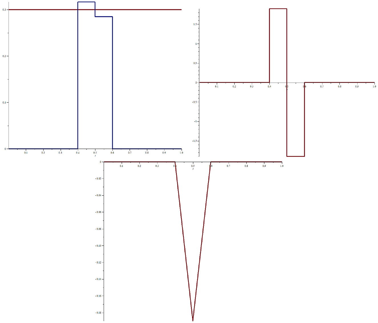
Figure 2. (Upper left) Bubble–antibubble pair as a function of time t = T − τ (blue curve) and the volatility σ (red curve). Note that the positive and negative bubbles are equidistant with respect to σ. (Upper right) Potential v in terms of t. (Lower figure) Arbitrage number in terms of t. Note that after the bubble–antibubble pair has finished acting, the arbitrage number is zero.

Figure 3 shows the effect of a bubble–antibubble pair on a call option with parameters K = 5, r = 0.1, and α = 0.2. The curve at τ = 0 (t = T = 1) is the usual contract function Φ(S) = max{0, S − K}. For 0 < τ ≤ τ₁, the dynamics are given by the free Black–Scholes solution. For τ₁ ≤ τ ≤ τ₂, the bubble acts and changes the dynamics to create an interacting solution. However, due to the fact that the arbitrage number of the bubble–antibubble pair is zero, for τ₂ ≤ τ ≤ T, the interacting dynamics are again given by the free Black–Scholes model. Thus, when the arbitrage number is zero, the bubble has no effect on the option at maturity.

FIGURE 3

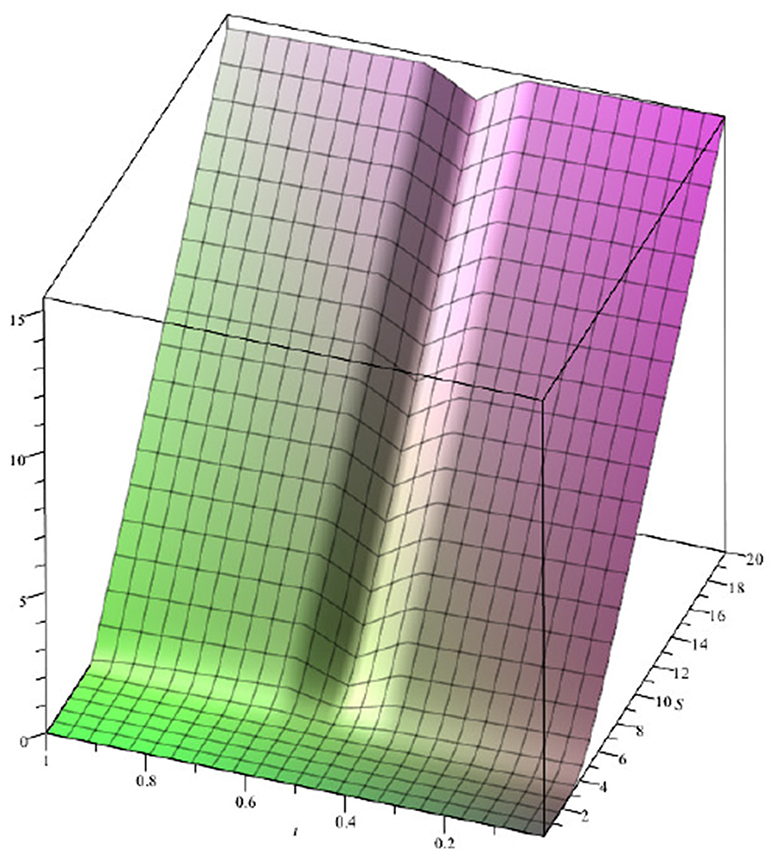
Figure 3. (Left) Effect of a bubble–antibubble pair on a call option. Note that for τ₂ ≤ τ ≤ T, the option recovers its free initial dynamics due to the fact that the bubble arbitrage number is 0.

Example 3: Consider the case of three successive square bubbles of the form,

$\begin{array}{ll}f(\tau )=\{\begin{array}{cc}0& 0\le \tau \le {\tau }_1,\\ f_0& {\tau }_1<\tau <{\tau }_2,\\ f_1& {\tau }_2<\tau <{\tau }_3,\\ f_2& {\tau }_3<\tau <{\tau }_4,\\ 0& {\tau }_4\le \tau \le T.\end{array}& (81)\end{array}$

Figure 4 shows the effect of two negative bubbles and one positive bubble (left figure), as well as that of one positive bubble and two negative bubbles (right figure), on a call option. In all cases, the total arbitrage number is zero. Here, K = 5, r = 0.1, σ = 0.3, T = 1, α = 0.2, τ₁ = 0.2, τ₂ = 0.4, τ₃ = 0.5, and τ₄ = 0.6. For the left figure, f₀ = 0.24, f₁ = 0.276, and f₂ = 0.316, whereas for the right figure, f₀ = 0.33, f₁ = 0.24, and f₂ = 0.28.

FIGURE 4

Figure 4. (Left) Effect of two negative bubbles and one positive bubble, respectively. (Right) Effect of one positive bubble and two negative bubbles. In all cases, the total arbitrage number is zero. Thus, the dynamics of the option at maturity are the usual free Black–Scholes dynamics.

Figure 5 shows the effect on a call option of one positive bubble, one negative bubble, and one positive bubble, respectively (left figure), and one negative bubble, one positive bubble, and one negative bubble, respectively (right figure). In all cases, the total arbitrage number is zero. Here, K = 5, r = 0.1, σ = 0.3, T = 1, α = 0.2, τ₁ = 0.2, τ₂ = 0.3, τ₃ = 0.5, and τ₄ = 0.6. For the left figure, f₀ = 0.345, f₁ = 0.273, and f₂ = 0.326, whereas for the right figure, f₀ = 0.27, f₁ = 0.33, and f₂ = 0.278.

FIGURE 5

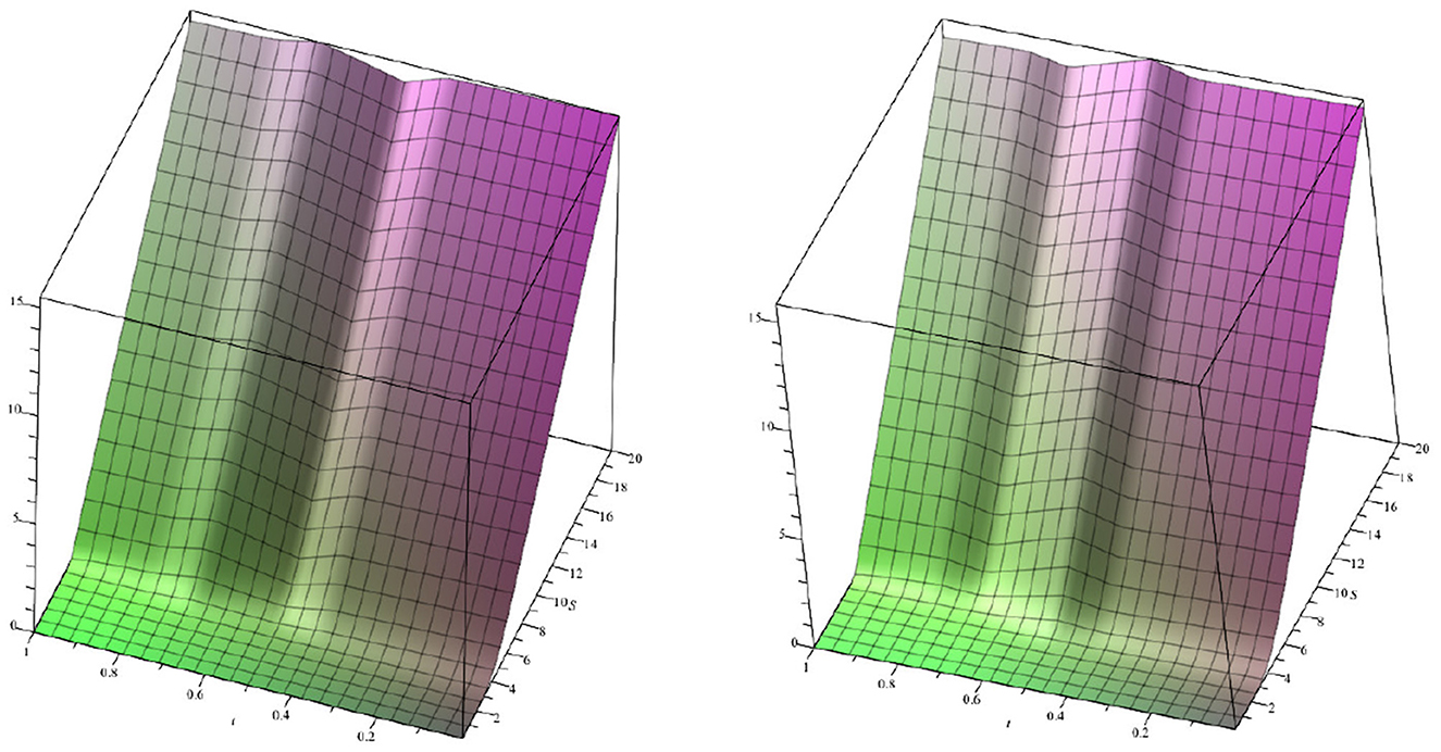
Figure 5. (Left) One positive bubble, one negative bubble, and one positive bubble. (Right) One negative bubble, one positive bubble, and one negative bubble. The total arbitrage number is zero. Note again that the dynamics of the option at maturity are the usual free Black–Scholes dynamics.

Figure 6 shows the effect on a call option of one positive bubble and two negative bubbles (left figure) and two negative bubbles and one positive bubble (right figure), but in this case, the total arbitrage number A_N ≠ 0. The parameters are the same as those used in Figure 5, but for the left figure, f₀ = 0.345, f₁ = 0.273, f₂ = 0.294, and A_N = −0.616, whereas for the right figure, f₀ = 0.273, f₁ = 0.285, f₂ = 0.3015, and A_N = 2.01. In this situation, the option dynamics at maturity are far away from the free dynamics. Thus, the bubble action has a net effect on the option price when A_N ≠ 0.

FIGURE 6

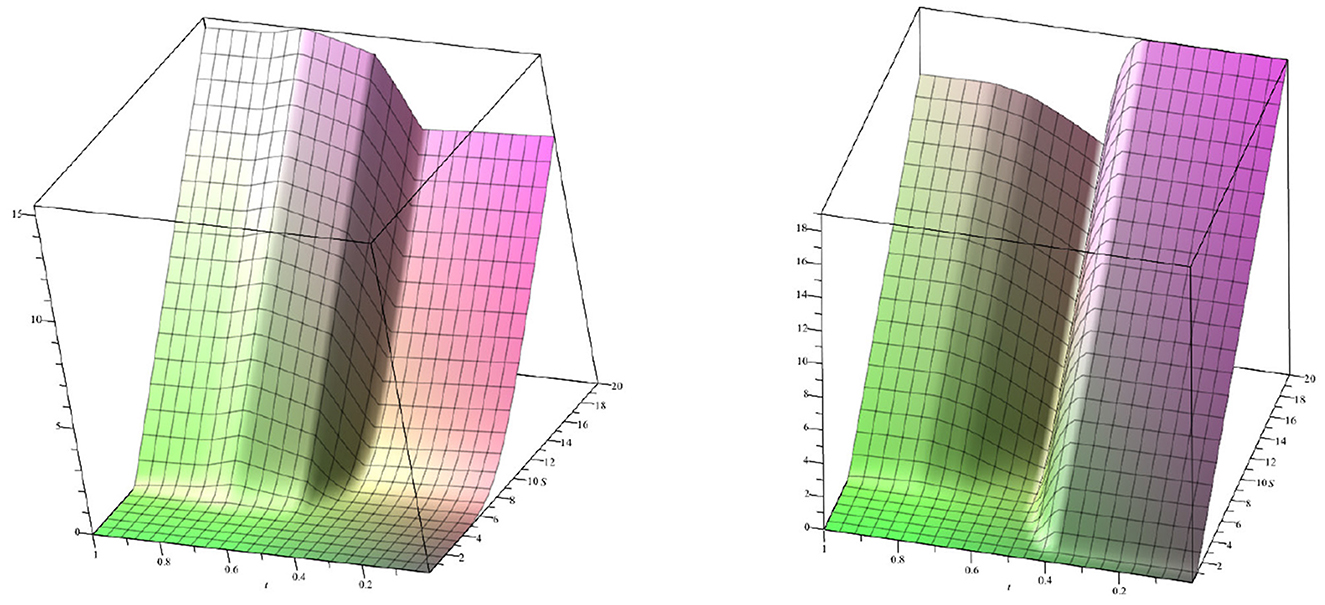
Figure 6. (Left) Effect of one positive bubble and two negative bubbles for a total arbitrage number A_N = −0.616. (Right) Effect of two negative bubbles and one positive bubble but with A_N = 1.529. Note that after the bubble acts, the evolution of the option does not follow the dynamics of the free model; instead, its behavior changes radically.

6. Conclusion

Three theorems about the exact dynamical behavior of the option price when time-dependent arbitrage bubbles are incorporated explicitly in the Black–Scholes equation have been presented. These arbitrage bubbles (which can act at some instant t between 0 and the maturity T) can be characterized by an arbitrage number A_N(τ) that corresponds to the accumulated external potential from time 0 to time τ. If A_N(t = 0) = 0 or A_N(τ = T) = 0, independent of the bubble's dynamic behavior, the option's values at maturity are given by the usual Black–Scholes dynamics with an interest rate r. In some sense, the option does not remember the past arbitrage process. If A_N(t = 0) ≠ 0 or A_N(τ = T) ≠ 0, the option price depends on the bubble and on all the higher derivatives (or Greeks) of the solution of the free Black–Scholes equation with an interest rate r, and it is equal to a solution of the free Black–Scholes equation with an interest rate r + (1/T)A_N(τ = T). In this case, the option remembers the past arbitrage processes.

Thus, arbitrage bubbles with A_N(t = 0) = 0 are innocuous because the system returns to the initial equilibrium state. However, bubbles with A_N(t = 0) ≠ 0 are dangerous from a financial point of view, because these bubbles change the initial equilibrium trajectory of the option price.

We hope that these theorems will make it easier to understand an option's dynamic evolution when arbitrage processes are included. A generalization of these theorems and their consequences, for the case of a price-dependent bubble f = f(S, t), will be studied in future research.

Data availability statement

The original contributions presented in the study are included in the article/Supplementary material, further inquiries can be directed to the corresponding author.

Author contributions

MC and RO: conceptualization, investigation and formal analysis, visualization, writing—original draft, and editing. All authors contributed to the article and approved the submitted version.

Acknowledgments

The authors would like to thank the Industrial Engineering School of Diego Portales University for its economic support of the article published in this journal.

Conflict of interest

The authors declare that the research was conducted in the absence of any commercial or financial relationships that could be construed as a potential conflict of interest.

Publisher's note

All claims expressed in this article are solely those of the authors and do not necessarily represent those of their affiliated organizations, or those of the publisher, the editors and the reviewers. Any product that may be evaluated in this article, or claim that may be made by its manufacturer, is not guaranteed or endorsed by the publisher.

Supplementary material

The Supplementary Material for this article can be found online at: https://www.frontiersin.org/articles/10.3389/fams.2023.1138663/full#supplementary-material

Footnotes

1. ^Using a martingale approach, other authors have investigated the effect of bubbles on the valuation of the underlying asset and derivative assets. See, for example, Jarrow and Kwok [30] and Benth et al. [31].

2. ^Note that C(S, t = 0, r) is the solution of the equilibrium Black–Scholes equation for any derivative asset.

References

1. Black F, Scholes M. The pricing of options and corporate liabilities. In: Galai D, Crouhy M, Wiener Z, editors. World Scientific Reference on Contingent Claims Analysis in Corporate Finance: Volume 1: Foundations of CCA and Equity Valuation. Singapore: World Scientific (2019), p. 3–21. doi: 10.1142/9789814759588_0001

CrossRef Full Text | Google Scholar

2. Merton RC. Theory of rational option pricing. Bell J. Econ. Manage. Sci. (1973) 4:141–83. doi: 10.2307/3003143

CrossRef Full Text | Google Scholar

3. Heston SL. A closed-form solution for options with stochastic volatility with applications to bond and currency options. Rev Financ Stud. (1993) 6:327–43. doi: 10.1093/rfs/6.2.327

CrossRef Full Text | Google Scholar

4. Gatheral J. The Volatility Surface. Hoboken, NJ: Wiley (2006).

Google Scholar

5. Wilmott P. Paul Wilmott on Quantitative Finance. Hoboken, NJ: Wiley (2000).

Google Scholar

6. Dupire B. Pricing with a smile. Risk. (1994) 7:18–20.

Google Scholar

7. Björk T. Arbitrage Theory in Continuous Time. Oxford: Oxford University Press (2009).

Google Scholar

8. Ho TS, Lee SB. Term structure movements and pricing interest rate contingent claims. J Finance. (1986) 41:1011–29. doi: 10.1111/j.1540-6261.1986.tb02528.x

PubMed Abstract | CrossRef Full Text | Google Scholar

9. Tankov P. Financial Modelling with Jump Processes. Boca Raton, FL: Chapman and Hall/CRC (2003). doi: 10.1201/9780203485217

CrossRef Full Text

10. Hull J. Options, Futures, and Other Derivative Securities, 2ed. Hoboken, NJ: Prentice Hall (1993).

11. Sofianos G. Index arbitrage profitability. J Deriv. (1993) 1:6–20. doi: 10.3905/jod.1993.407871

CrossRef Full Text | Google Scholar

12. Lo AW, MacKinlay AC. A Non-Random Walk Down Wall Street. Princeton, NJ: Princeton University Press (1999).

Google Scholar

13. Ilinski K. Physics of Finance: Gauge Modelling in Non-Equilibrium Pricing. Hoboken, NJ: John Wiley & Sons Inc (2001).

Google Scholar

14. Adrian T. Inference, arbitrage, and asset price volatility. J Financ Intermed. (2009) 18:49–64. doi: 10.1016/j.jfi.2008.06.001

CrossRef Full Text | Google Scholar

15. Cornell B, French KR. Taxes and the pricing of stock index futures. J Finance. (1983) 38:675–94. doi: 10.1111/j.1540-6261.1983.tb02496.x

CrossRef Full Text | Google Scholar

16. Figlewski S. Hedging performance and basis risk in stock index futures. J Finance. (1984) 39:657–69. doi: 10.1111/j.1540-6261.1984.tb03654.x

CrossRef Full Text | Google Scholar

17. Stoll HR, Whaley RE. Program trading and expiration-day effects. Financ Anal J. (1987) 43:16–28. doi: 10.2469/faj.v43.n2.16

CrossRef Full Text | Google Scholar

18. Brennan MJ, Schwartz ES. Arbitrage in stock index futures. J Bus. (1990) 63:S7–S31. doi: 10.1086/296491

CrossRef Full Text | Google Scholar

19. Ilinski K. Virtual arbitrage pricing theory. arXiv. (1999) [preprint]. doi: 10.48550/arXiv.cond-mat/9902045

CrossRef Full Text | Google Scholar

20. Ross SA. The arbitrage pricing theory of capital asset pricing. J Econ Theory. (1976) 13:334–60. doi: 10.1016/0022-0531(76)90046-6

PubMed Abstract | CrossRef Full Text | Google Scholar

21. Elton EJ, Gruber MJ. Modern Portfolio Theory and Investment Analysis. Hoboken, NJ: John Wiley & Sons (1995).

22. Ilinski K. Physics of finance. In: Kertesz J, Kondor I, editors. Econophysics: An Emerging Science. Philadelphia, PA: Kluwer (1998).

Google Scholar

23. Callen HB. Thermodynamics. Hoboken, NJ: John Wiley & Sons (1960).

Google Scholar

24. Ilinski K. How to account for virtual arbitrage in the standard derivative pricing. arXiv. (1999) [preprint]. doi: 10.48550/arXiv.cond-mat/9902047

CrossRef Full Text | Google Scholar

25. Ilinski K, Stepanenko A. Derivative pricing with virtual arbitrage. arXiv. (1999) [preprint]. doi: 10.48550/arXiv.cond-mat/9902046

CrossRef Full Text | Google Scholar

26. Panayides S. Arbitrage opportunities and their implications to derivative hedging. Phys A: Stat Mech Appl. (2006) 361:289–96. doi: 10.1016/j.physa.2005.06.077

CrossRef Full Text | Google Scholar

27. Panayides S, Fedotov S. Stochastic arbitrage return and its implication for option pricing. Phys A: Stat Mech Appl. (2005) 345:207–17. doi: 10.1016/S0378-4371(04)00989-6

CrossRef Full Text | Google Scholar

28. Papanicolaou GC, Sircar KR. Stochastic volatility, smiles and asymptotics. Appl Math Finance. (1999) 6:107–45. doi: 10.1080/135048699334573

CrossRef Full Text | Google Scholar

29. Contreras M, Montalva R, Pellicer R, Villena M. Dynamic option pricing with endogenous stochastic arbitrage. Phys A: Stat Mech Appl. (2010) 389:3552–64. doi: 10.1016/j.physa.2010.04.019

CrossRef Full Text | Google Scholar

30. Jarrow RA, Kwok SS. Inferring Financial Bubbles from Option Data. School of Economics, University of Sydney (2020). Available online at: https://ideas.repec.org/p/syd/wpaper/2020-04.html

Google Scholar

31. Benth FE, Crisan D, Guasoni P, Manolarakis K, Muhle-Karbe J, Nee C, et al. A mathematical theory of financial bubbles. In: Henderson V, Sircar R, editors. Paris-Princeton Lectures on Mathematical Finance 2013. New York, NY: Springer (2013), p. 1–108. doi: 10.1007/978-3-319-00413-6

CrossRef Full Text | Google Scholar

32. Heston SL, Loewenstein M, Willard GA. Options and bubbles. Rev Financ Stud. (2007) 20:359–90. doi: 10.1093/rfs/hhl005

CrossRef Full Text | Google Scholar

33. Jarrow RA. Asset price bubbles. Ann Rev Financ Econ. (2015) 7:201–18. doi: 10.1146/annurev-financial-030215-035912

CrossRef Full Text | Google Scholar

34. Contreras M, Pellicer R, Santiagos D, Villena M. Calibration and simulation of arbitrage effects in a non-equilibrium quantum Black-Scholes model by using semiclassical methods. J Math Finance. (2016) 6:541–61. doi: 10.4236/jmf.2016.64042

CrossRef Full Text | Google Scholar

35. Contreras M, Pellicer R, Villena M, Ruiz A. A quantum model of option pricing: when Black-Scholes meets Schrödinger and its semi-classical limit. Phys A: Stat Mech Appl. (2010) 389:5447–59. doi: 10.1016/j.physa.2010.08.018

CrossRef Full Text | Google Scholar

36. Merzbacher E. Quantum Mechanics. Hoboken, NJ: Wiley. (1998).

Google Scholar

37. Sakurai J, Napolitano J. Modern Quantum Mechanics, 2nd ed. San Francisco, CA: Pearson. (2011).

Google Scholar