 Abdulai Kailan Suhuyini
 Baba Seidu
- Department of Mathematics, School of Mathematical Sciences, C. K. Tedam University of Technology and Applied Sciences, Navrongo, Ghana
Typhoid fever is a potentially fatal illness that is caused by the bacteria Salmonella typhi. In this study, a deterministic mathematical model was formulated to look into transmission dynamics of typhoid fever with treatment and booster vaccination. The reproduction number is calculated using the next-generation matrix approach. Then, a stability analysis on the equilibrium points was performed using Routh–Hurwitz criteria. It was revealed that the disease-free equilibrium point is locally asymptotically stable whenever is less than 1 together with other conditions. We also showed that does not guarantee global stability of the typhoid-free equilibrium point and corroborated the result by showing the possible existence of backward bifurcation at . The model parameters in were also subjected to sensitivity analysis, which revealed that the transmission rate, infection through an exposed person, and bacteria are the most influential parameters of the reproduction number . Numerical simulations were run to determine the impact of various parameters on the dynamics of typhoid.
1. Introduction
Typhoid fever, also known as enteric fever, is an enfeebling infectious disease that infects humans. It is normally high in children below the age of 6 years of age and is relatively average in adults. Bacteria, known as Salmonella typhi (S. typhi), are the primary cause of typhoid fever. The disease is usually contracted by infecting humans through the intake of fecal discharges from an infected person, contaminated water or food, and by sharing basic utensils, such as cups, spoons, bowls, and others, with an infected person. Some express it bluntly by saying that a person who has contracted typhoid fever has eaten the feces of a carrier or another infected person. These gram-negative bacteria find their way into the body through the aforementioned ways into the small intestine and then shed into the bloodstream by macrophages in the reticuloendothelial system [1]. The symptoms of typhoid fever include prolonged low to high fever, severe headache, loss of appetite, body pain and weight loss, dry cough, diarrhea or constipation, itching or rashes, and also, to some extent nausea, and abdominal pain. At the chronic stage of typhoid, perforation of the intestine and neurological complications are observed in the patient [2]. Endemic cases of typhoid fever are recorded in both developed and developing countries, thereby making it a public health concern. This disease still remains a concern, even despite the recent improvements in water sanitation [3]. Usually, it takes 7–14 days for the disease to manifest in an infected person. The patient is given antibiotic treatment, after which the person may feel better a few days later. Still, in the worse case, an infected person without a proper treatment could develop complications resulting in death. Vaccines against typhoid fever are only partially effective. The said vaccines are usually manufactured only for those persons who are prone or are exposed to hotspot areas of the disease [4]. Hence, the jabs of typhoid fever vaccines are seen as one of the core factors in curbing the transmission of the disease. The available vaccines in the system now are of two types that are oral and injectable. Among the injectable types, we have: typhoid conjugate vaccine, Tya, and Vi capsular polysaccharide vaccine. They are about 30% to 80% effective within the first 2 years of the specific vaccine in question. When a person takes on the drug-resistant strain of typhoid fever and is not properly managed with effective antibiotics, then there is a high chance of it resulting in complications [5]. It is estimated that typhoid fever cases have risen from 11 million to 21.5 million and five million cases of paratyphoid fever worldwide, with 200,000 deaths occurring each year [6]. It is also estimated that African countries have not been left out with an increasing number of cases between 10 and 100 per 100,000 individuals, with children being the most infected due to poor hygiene and sanitation. As a result of the high rate of infection and the rising spirit of the disease strain, typhoid has become a burden that has turned into a major world health problem. However, vaccination seems to be the essential method for controlling the transmission of the disease [7]. Several mathematical models have been proposed to study the dynamics of infectious diseases. Among the diseases that have gained much attention from mathematical modelers are HIV/AIDS [8–10, and references therein], malaria [11, and references therein], and tuberculosis [12, and references therein]. With the advent of coronavirus disease (COVID-19), several models have been proposed to study the dynamics and control of the disease [13, 14, and references therein]. González-Guzmán [15] appears to be from among the first researchers to have developed a mathematical model to study the spread of typhoid fever. Following González-Guzmán [15], several models have been proposed to help increase the understanding of the spread and control of typhoid fever. Specifically, Wameko et al. [16] proposed a deterministic ODE compartmental model for the dynamics of typhoid fever with a susceptible-carrier-infected-recovered (ESCIR) pattern for the human population and a pathogen compartment B(t). The recent study of Ayoola et al. [17] analyzed a similar compartmental model for the spread of typhoid fever by incorporating optimal education and vaccination control strategies. A six-class compartmental model by Ogunlade et al. [18] describes the application of deterministic and stochastic models to the dynamics of typhoid fever. They first analyzed the deterministic model and then transformed it into a stochastic model where the mean and variance were determined. The stochastic model simulations were done using the Euler–Maruyama numerical scheme. Even though the research indicates that controls, such as vaccination, screening, and treatments, are effective enough to reduce the spread of the disease, hospitalization and personal hygiene could not be considered to help control the disease. Other interesting models of typhoid fever can be seen in Peter et al. [19], Peter et al. [20, 21], and Musa et al. [7].
To the best of our knowledge, no typhoid fever model that incorporates treatment and booster vaccination as control measures has been proposed. Therefore, this research seeks to develop a mathematical fever model that incorporates vaccination, treatment, booster vaccine, and pathogen populations.
The rest of the article is arranged as follows: In Section 2, the model of interest is formulated. In Section 3, basic qualitative properties, including positivity and boundedness of model solutions, stability of equilibrium points of the model, are discussed. In Section 4, the model is numerically simulated to illustrate the analytical results obtained and to study the impact of model parameters on model output behavior. Finally, in Section 5, the main conclusions drawn from the study are presented.
2. Formulation of the mathematical model
Based on the model proposed by Ayoola et al. [17], we incorporate double-dose vaccination with treatment and a compartment to monitor the concentration of the bacteria in the environment. The said model consists of six human compartments and one pathogen compartment. These are: the singly vaccinated population V, the susceptible population, S, the exposed E, infected, I, recovered R, and those who have received the booster vaccine VB. The pathogen concentration is given by B. Therefore, the total human population is given by N = V + S + E + I + R + VB + B. The susceptible represents the people who are uninfected but stand the chance of getting infected with the disease. This compartment increases through the following:
• Recruitment at rate nΛh, where Λh is the recruitment rate into the population and n is the proportion of the recruits who are susceptible,
• Loss of immunity of the single-vaccinated individuals. The rate of loss of immunity by the single-vaccinated individuals is taken to be ν1, The recovered population may lose their temporal immunity and join the susceptible at rate θ.
The susceptible population also reduces due to the following:
• Infection as a result of effective contact with the exposed and infected persons at the rate of (1 − η)βSλ, where λ = β(γ1E + γ2I + γ3B). A proportion η of those susceptible become exposed, while the remainder become infectious right away due to compromised immune system,
• Vaccination at rate ϕ.
• Natural death at rate μ.
The single-dose vaccinated population increases through recruitment at a rate (1 − η)Λh, vaccination of the susceptible and recovered at rates of ν1, and ν2, respectively. The vaccinated population also reduces as a result of: the loss of immunity at rate ϕ, going in for booster vaccine at a rate ρ, and through natural death at a rate μ. The exposed compartment increases through some fraction η of susceptible population following effective contact with infected, exposed persons and the pathogen at a rate ηSλ, and decreases as a result of the natural recovery rate of w, the natural mortality rate of μ, and the development of clinical symptoms at a rate of ψ. The infected compartment grows through infection following the effective contact with exposed, infected persons and the shed pathogen in the environment at rate (1 − η)λS, and progression of exposed individuals into the infected class at rate ψ. The infected population diminishes in the following manner: a successful treatment at rate τ, a disease-induced mortality at rate of δ, and natural mortality rate of μ. The recovered compartment population increases through a successful treatment of infected persons at the rate of τ and natural self-recovery of the exposed at the rate of w. The recovered compartment also reduces as a result of temporal immunity loss at the rate θ, rate of vaccination ν2, and natural mortality rate μ. The booster vaccinated compartment grows through the intake of booster vaccine by the vaccinated compartment at the rate ρ and reduces as a result of the natural mortality rate μ and the Pathogen concentration increases through the shedding of pathogens by exposed and infectious persons at rates ξ1 and ξ2, respectively. The decay rate of pathogens is taken to be μb.
The schematic diagram that represents the model described thus far is presented in Figure 1.
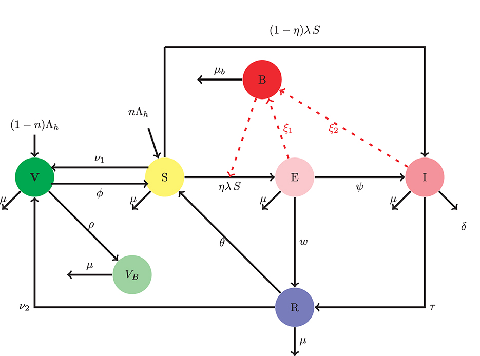
Figure 1. Compartmental diagram of the model.
The following set of differential equations therefore describes the dynamics of typhoid spread with double-dose vaccination scheme:
Where necessary, we use the following conventions in subsequent discussions.
In Table 1, the model parameters and their baseline values are presented.
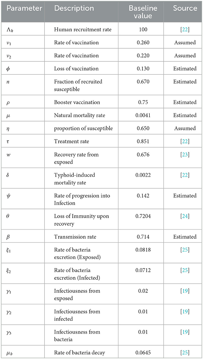
Table 1. Description and values of parameters for model (Equation 1).
3. Qualitative properties
3.1. Positivity of solutions
Theorem 1. Let . If positive conditions and initial conditions are provided for Equation (1), then all its solutions remain positive for t > 1.
Thus, V(t) > 0, S(t) ≥ 0, E(t) ≥ 0, I(t) ≥ 0, R(t) ≥ 0, VB(t) ≥ 0, B(t) ≥ 0 of the system is positive for all t > 1.
Proof. Considering the first of Equation (1), we have
Integrating both sides gives
Where C1 is the integration constant, i.e., V(0) = C1. Therefore, V(0) ≥ 0 ∀ t > 0. □
Similarly, we can show this for {S(0) ≥ 0, E(0) ≥ 0, I(0) ≥ 0, R(0) ≥ 0, VB(0) ≥ 0, B(0) ≥ 0} model variables. As a result, the model's solution is positive.
3.2. Boundedness of solutions
Adding all equations consisting of human compartments from model system (1) gives;
Solving Equation (2) yields
Now,
Thus, N(t) is bounded.
With use of the inequality (Equation 3), we obtained from the seventh equation of system (Equation 1) that,
Solving inequality (Equation 4), we have
Taking the limits will give
Hence, B(t) is bounded as well. Thus, the aforementioned results indicate that the solutions of system (Equation 1) are positive and bounded in the region.
3.3. Equilibrium points of model
3.3.1. Typhoid-free equilibrium point and basic reproduction number
The typhoid-free equilibrium is obtained by equating the dynamic system of Equation (1) to zero together with the conditions E = 0, I = 0, R = 0, and B = 0. Then, we have;
The basic reproduction number, which is often denoted by , is an epidemiological quantity which is used to describe the average number of secondary infections that are recorded as a result of introducing an infected individual into an otherwise completely susceptible population. Several techniques have been developed to determine this threshold for deterministic ODE models. In this article, we employ the method of Driessche et al. [26] to obtain for the typhoid fever model. Following the technique in Driessche et al. [26], the infected sub-system of model system (Equation 1) is given by the following set of equations.
According to Driessche and Watmough [26], the, matrix F represents the component consisting of the infection terms (transmission) and V contains all other terms (transitions). The transmission and transition matrices are then given by
Therefore,
Where ζ1 = μb(γ1k4 + γ2ψ) + γ3(ψξ2 + ξ1k4).
It is easy to determine that the basic reproduction number taken as the spectral radius of [26] is given by
3.3.2. Endemic equilibrium point
At a typical non-trivial equilibrium point , we have the following.
Solving the set of equations above, the endemic equilibrium point can be explicitly expressed in terms of λ* and other model parameters as follows:
Where
Substituting E*, I*, and B* into (10) and simplifying give
Solutions of Equation (11) are λ* = 0, corresponding to the typhoid-free equilibrium, and , corresponding to the typhoid-persistent equilibrium. The following result is easily established.
Lemma 1. The typhoid fever model (Equation 12) has an epidemiologically reasonable disease-free equilibrium point only when .
Proof. It is easy to notice that by substituting the expressions for k1, k2, … k5, and simplifying. This implies that the λ* > 0 if and λ* ≤ 0 if . We note that λ* > 0 is associated with a positive endemic equilibrium. This concludes the proof. □
3.4. Stability of equilibrium points
We investigate the local stability of the typhoid-free equilibrium and the endemic equilibrium of the basic reproduction number, in this section, using the Lyapunov second technique, which states that an equilibrium point is locally asymptotically stable if all eigenvalues of the associated Jacobian have negative real parts and unstable otherwise.
3.4.1. Local stability of equilibrium points
The typhoid-free equilibrium is locally asymptotically stable, if and only if all eigenvalues of the Jacobian matrix of system (Equation 1) at the have negative real parts. Now, let X = (S, E, I, R, V, VB, B). Then, model (Equation 1) can be written in the form , where , where Xi is the ith component of X.
The Jacobian matrix of the model evaluated at typhoid-free equilibrium we have is given by
If Y is a typical eigenvalue, then the characteristic polynomial of is given by
where
Clearly, two of the eigenvalues of , namely, −μ and −k are negative. Two other eigenvalues can be determined as,
which clearly have negative real parts since (k1k2 − ν1ϕ) > 0, and (k1 + k2) > 0. Now, the condition for stability of typhoid-free equilibrium point rests on the zeros of Ψ(Y). These roots have negative real parts if Δ1 > 0, Δ2 > 0, Δ3 > 0, and Δ1Δ2 > Δ3.Clearly, Δ3 > 0 whenever . Therefore, the local stability of is characterized in the following result.
Lemma 2. The typhoid-free equilibrium point is locally asymptotically stable whenever and the conditions Δ1 > 0, Δ2 > 0, and Δ1Δ2 > Δ3 also hold. The equilibrium point is unstable otherwise.
3.5. Global stability of typhoid-free equilibrium points
To study the global stability of the typhoid-free equilibrium point, we define the Lyapunov function
The time derivative of is given by
Upon substituting the expressions for , and into the aforementioned equation and simplifying, we obtain the following.
Now, and hence, if . Therefore, even though is required for local stability, it is not sufficient for global stability. This suggests the existence of backward bifurcation, which will be explored in the next section.
3.6. Sensitivity analysis
Mathematical models have always been proposed and used to make predictions. The reliability of the predictions from these models depends not only on the precision or accuracy of the models, but also on the precision or accuracy of the model inputs, which are mostly in the form of model parameters. Data on these model parameters are often uncertain. Thus, the measurement of model parameters can affect predictions by models. It is therefore important to study the impact of variations in model parameters on the model output. This is done through sensitivity analysis. In this section, we adopt the forward normalized sensitivity index to study the effect of small changes in model parameters on model predictions. This index allows us to determine the parameters with the maximum impact on the model output, so that these models can be targeted for an accurate or precise measurement and also to optimize model predictions. The normalized sensitivity index is defined as follows:
Where z is an output that depends differentiably on the model input p. Using this index, we determined the sensitivity indices of endemic equilibrium and the basic reproduction number and evaluated them using the model parameter values given in Table 1. The sensitivity indices are presented in Table 2.
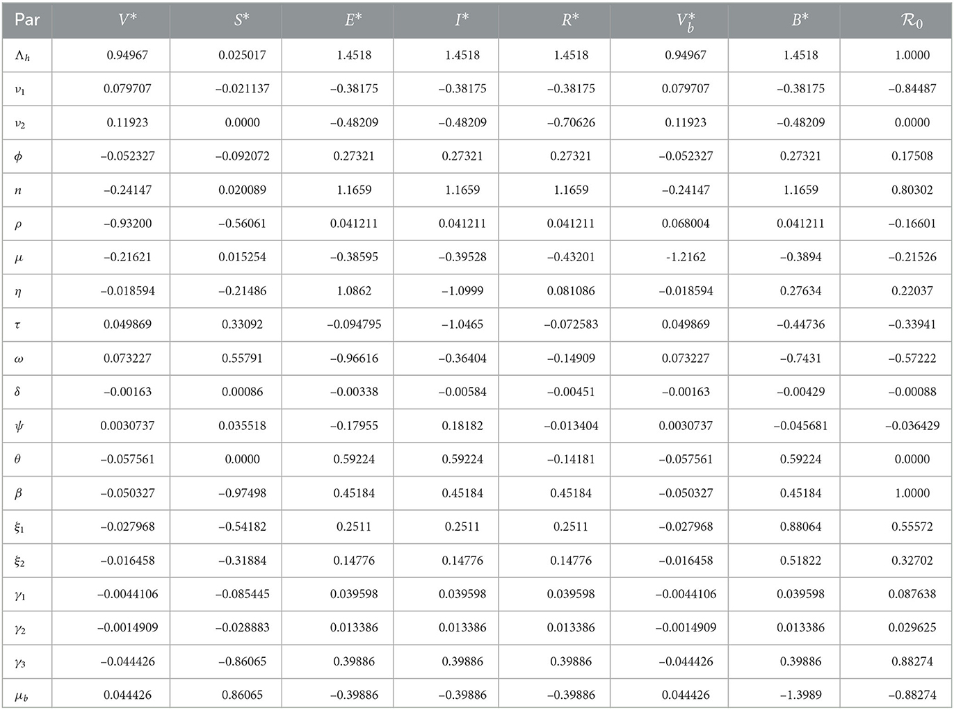
Table 2. Sensitivity indices of endemic equilibrium and .
The sensitivity indices indicate the percentage change in the given model output that follows from a percentage change in the model input. Positive indices indicate that a percentage increase (decrease) in the model input leads to a corresponding decrease (increase) in the model output. The graphs in Figure 2 present the sensitivity indices.
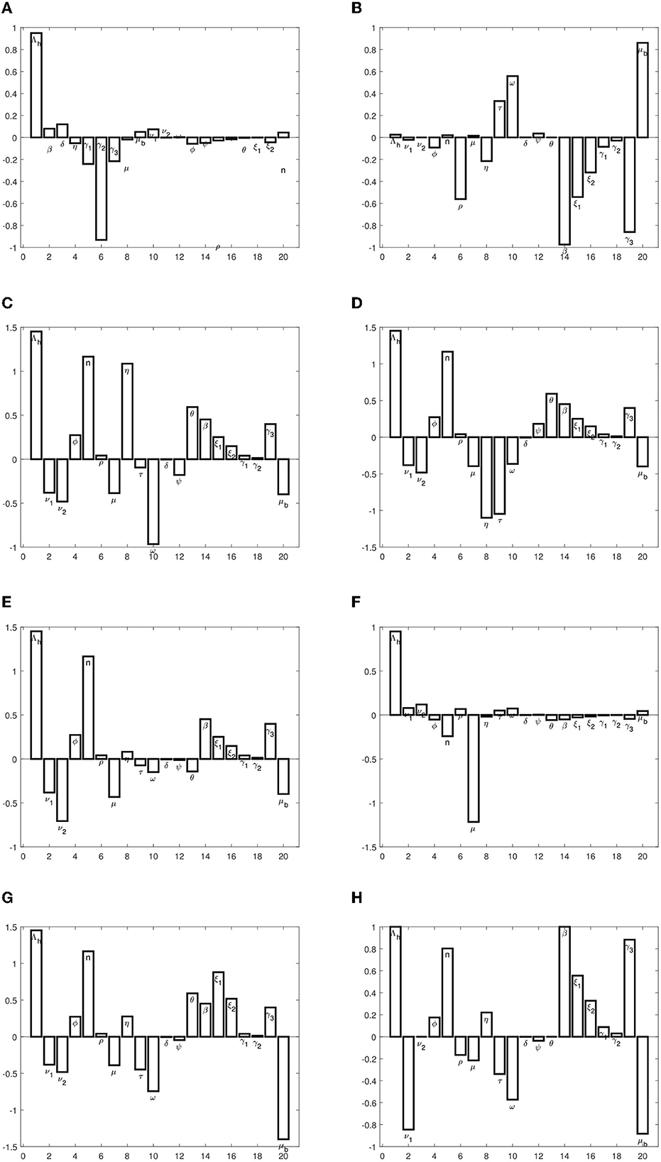
Figure 2. (A–H) Graphs of sensitivity indices of endemic equilibrium point, and .
We observe that the recruitment rate, Λh, has a high impact on all, except the susceptible population at equilibrium. The proportion of immigrants who are susceptible also has a high impact on exposed and infected populations. This implies that the inflow of persons into the population should be checked, so as to ensure that they are all vaccinated against typhoid. The transmission rate, β, also has a high impact on disease progression. We also observe that the rate at which individuals who come into contact with the pathogen sources remain exposed and not become infected has a high impact on disease spread. These parameters should be targeted to ensure that they are reduced or increased (whichever is appropriate) to keep the infections low. Specifically, to reduce or eradicate typhoid, the following measures should be carried out:
• The parameters, Λh,ϕ, n, β, ξ1, ξ2, γ1, γ2, and γ3, should be reduced.
• The parameters, ν1, μ, τ, ω, δ, ψ, and μb, should be increased.
We note however that increasing death rate in humans is not a good option and should hence be ignored.
3.7. Bifurcation analysis
In this section, we study the existence and direction of bifurcation in model (Equation 1). It is easy to show that the Jacobian of the model evaluated at the typhoid-free equilibrium point has a simple eigenvalue (i.e., a zero eigenvalue) when . Therefore, the center manifold theory [27] can be employed to study the nature of the bifurcation of the model.
To do this, we set x1 = V, x2 = S, x3 = E, x4 = I, x5 = R, x6 = VB, and x7 = B, so that the model can be written as follows:
The left and right eigenvectors (v and w, respectively) associated with the simple eigenvalue are given as follows:
Taking
as a bifurcation parameter, the nature and direction of bifurcation are determined by the bifurcation coefficients defined by
Direct computation and simplification yield the following.
where w4 and v4 satisfy
Since the signs of the bifurcation coefficients are not clearly known, the system exhibits backward bifurcation at whenever a > 0 and b > 0 [27].
4. Numerical simulation
In this section, we perform numerical simulations of the proposed model (Equation 1). The dynamic model system is simulated using the ode45 routine in MATLAB. The initial conditions used are given by
The the parameter values listed in Table 1 were used in the simulation. The simulation was performed to demonstrate the impact of each parameter on the transmission of typhoid fever. Contour plots, showing the impact of various parameters on the basic reproduction number , are presented in Figure 3.
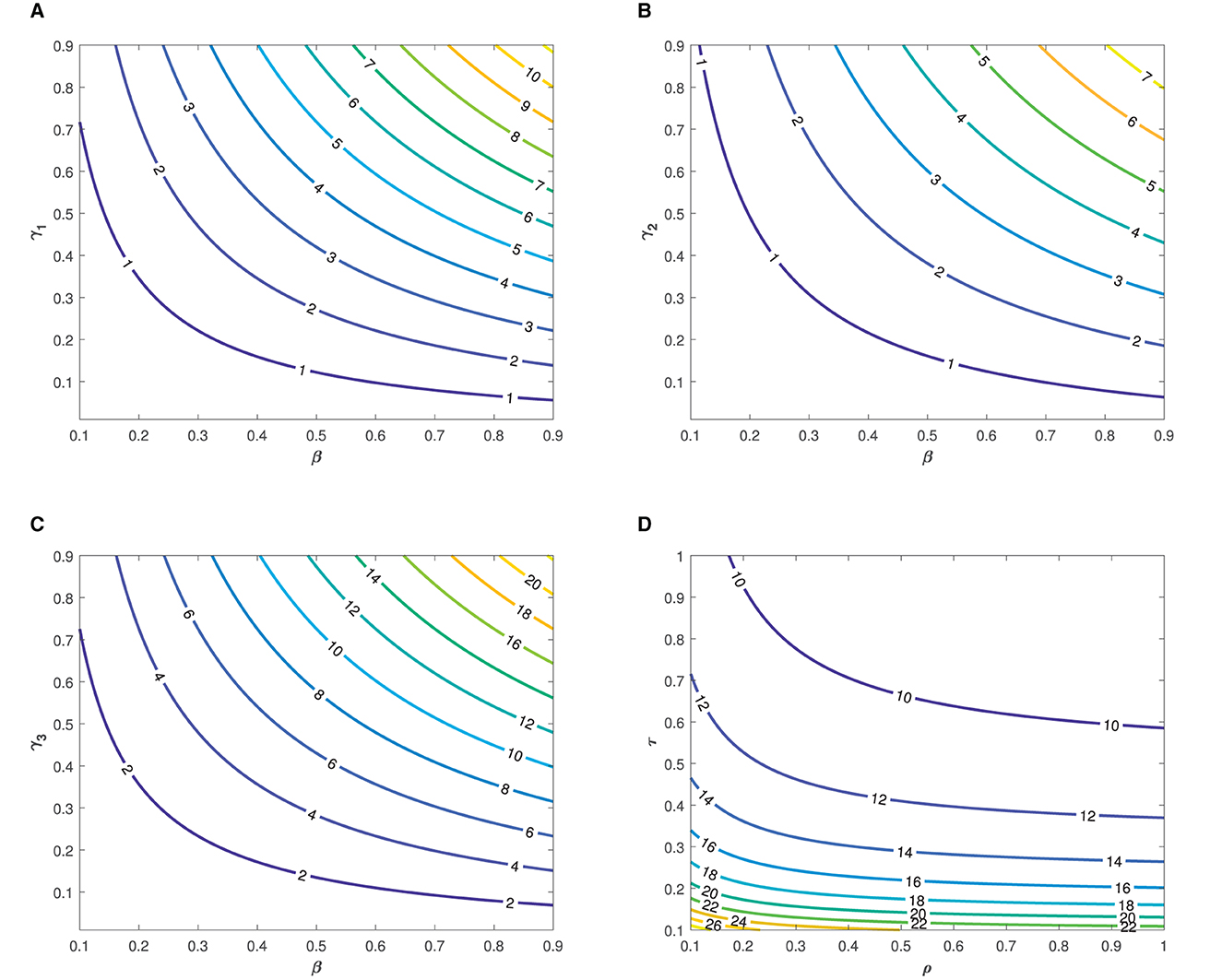
Figure 3. Contour plots showing the impact of various parameters on the basic reproduction number as functions of (A, B), β and γ2, (C) β and γ3, and (D) τ and ρ.
In Figure 4, the time series plots of model variables, showing the impact of varying the rate of administration of the first dose of typhoid vaccine, are presented. It is observed that increasing the rate of vaccine administration has the potential of driving infections downward. A similar effect of booster vaccine administration is observed from Figure the time series plots given in Figure 5. However, the booster vaccine is observed to have a far lesser impact on driving infections than the single dose. In Figure 6, the time series plots of model variables for varying values of the treatment rate are presented. It is observed that increasing the treatment rate has a very significant impact on infections but not so much for the other compartments. In Figure 7, time series plots showing the impact of loss of immunity after the first vaccination are presented. It is observed that an increased loss of immunity leads to an increase in the susceptible population and an increase in the Infected population.
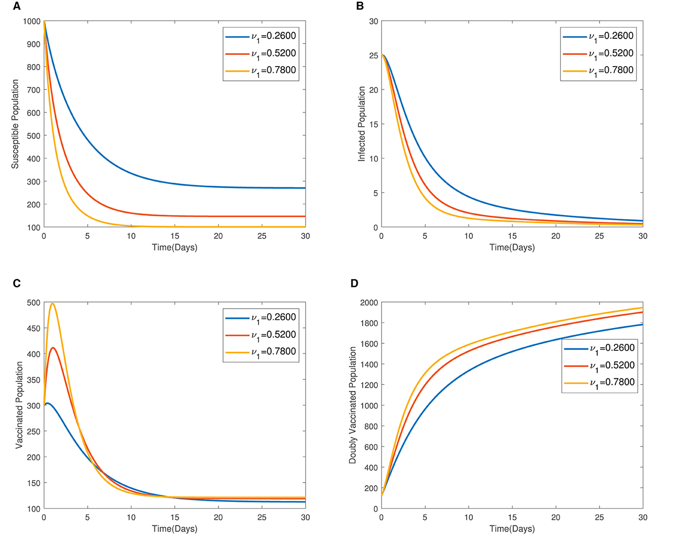
Figure 4. (A–D) Time series plots of model variables showing the impact of varying the rate of administration of the first dose of vaccine.
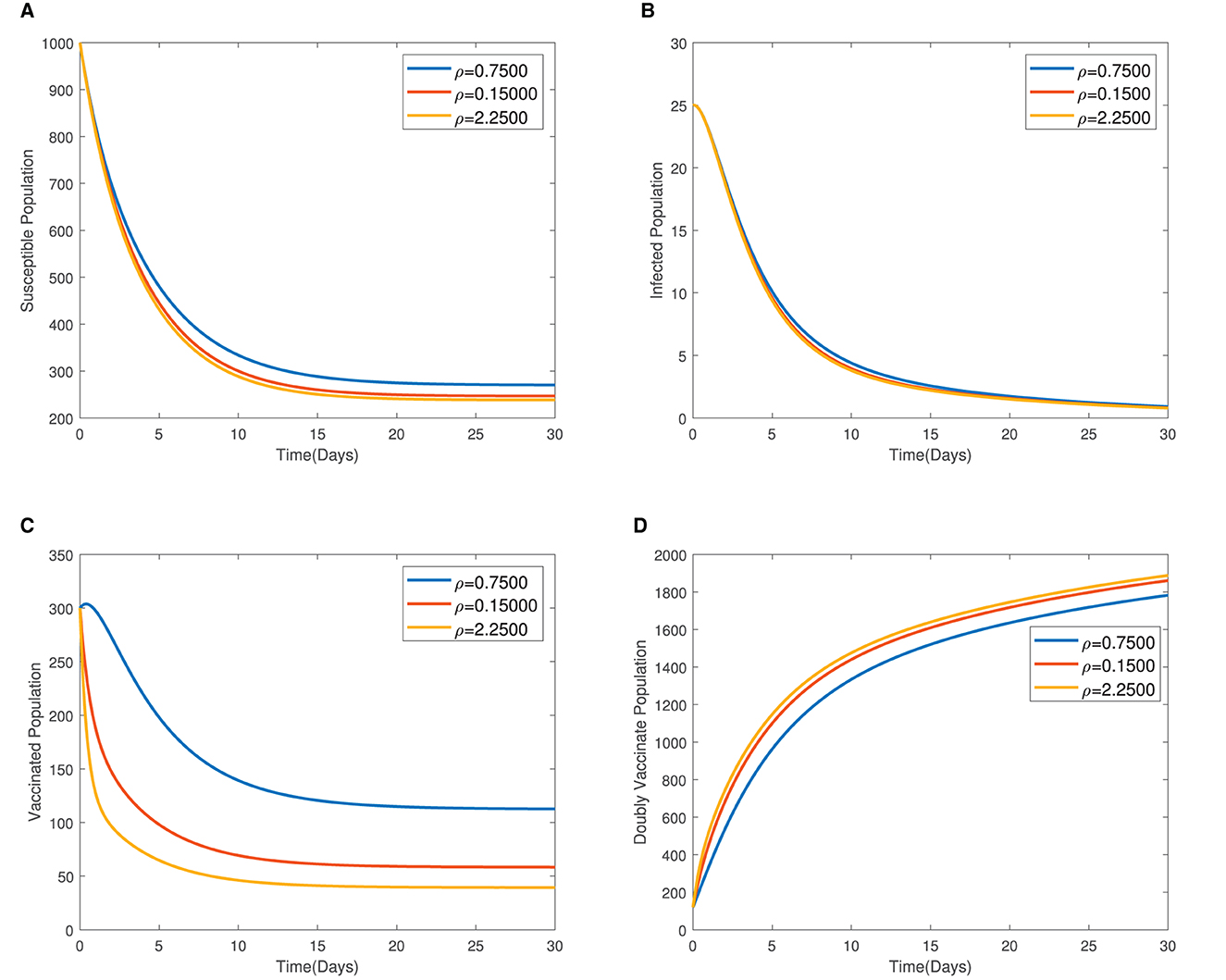
Figure 5. (A–D) Time series plots showing the impact of administration of the booster dose of vaccine.
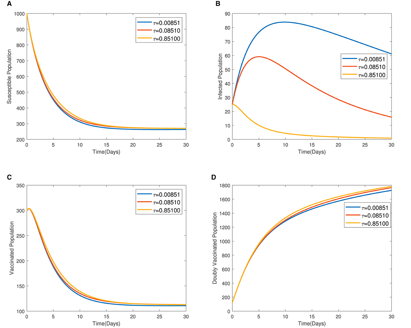
Figure 6. (A–D) Time series plots of model variables for varying values showing the impact of treatment rate.
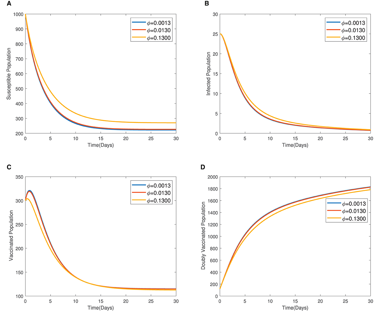
Figure 7. (A–D) Time series plots showing the impact of loss of immunity after the first vaccination.
5. Conclusions
This study formulated and analyzed a mathematical model for the transmission dynamics of typhoid fever disease, taking into account, both the booster vaccination and treatment. The region within which the analysis of the model is reasonable was determined. The typhoid-free and endemic equilibrium points were also determined. The basic reproduction number, , was then calculated using the next-generation matrix method of Driessche and Watmough [26]. The local and global stability conditions for the equilibrium points were investigated. We demonstrated that the model may exhibit backward bifurcation when under some conditions. Therefore, the condition may not be sufficient to eradicate typhoid fever in the community. A sensitivity analysis of the model parameters was conducted to determine the relative impact of changes in those model parameters on endemic equilibrium values and . It was observed that the most influential parameters include the transmission rate, β, recruitment rate, Λh, and the fraction of recruits who are susceptible, n. A numerical simulation was then conducted to illustrate the impact of various model parameters on the state variables. The results largely agree with the sensitivity index results. However, the results show that the booster vaccination may not be very effective in endemic areas.
Data availability statement
The original contributions presented in the study are included in the article/supplementary material, further inquiries can be directed to the corresponding author.
Author contributions
All authors listed have made a substantial, direct, and intellectual contribution to the work and approved it for publication.
Acknowledgments
This article was produced from the M.Phil. thesis of the first author under supervision of the co-author.
Conflict of interest
The authors declare that the research was conducted in the absence of any commercial or financial relationships that could be construed as a potential conflict of interest.
Publisher's note
All claims expressed in this article are solely those of the authors and do not necessarily represent those of their affiliated organizations, or those of the publisher, the editors and the reviewers. Any product that may be evaluated in this article, or claim that may be made by its manufacturer, is not guaranteed or endorsed by the publisher.
References
1. Parry CM, Hien TT, Dougan G, White NJ, Farrar JJ. Typhoid fever. N Engl J Med. (2002) 347:1770–82. doi: 10.1056/NEJMra020201
2. Antillón M, Warren JL, Crawford FW, Weinberger DM, Kürüm E, Pak GD, et al. The burden of typhoid fever in low- and middle-income countries: a meta-regression approach. PLoS Neglect Trop Dis. (2017) 11:e0005376. doi: 10.1371/journal.pntd.0005376
3. Dougan Baker GS. Salmonella enterica serovar typhi and the pathogenesis of typhoid fever. Ann Rev Microbiol. (2014) 68:317–36. doi: 10.1146/annurev-micro-091313-103739
4. Näsström E. Diagnosis of acute and chronic enteric fever using metabolomics (Ph.D. thesis). Umeå Universitet (2017).
5. Nthiiri J, Lawi G, Akinyi C, Oganga D, Muriuki W, Musyoka M, et al. Mathematical modelling of typhoid fever disease incorporating protection against infection. J Adv Math Comput Sci. (2016) 14:1–10. doi: 10.9734/BJMCS/2016/23325
6. CDC-US X. Typhoid and Paratyphoid fever: Information for Healthcare Professionals. Washington, DC: U.S. Department of Health and Human Services (2019).
7. Musa SS, Zhao S, Hussaini N, Usaini S, He D. Dynamics analysis of typhoid fever with public health education programs and final epidemic size relation. Results Appl Math. (2021) 10:100153. doi: 10.1016/j.rinam.2021.100153
8. Daabo MI, Makinde OD, Seidu B. Modeling the combined effects of careless susceptible and infective immigrants on the transmission dynamics of hiv/aids epidemics. J Public Health Epidemiol. (2013) 5:362–9.
9. Daabo MI, Makinde OD, Seidu B. Modelling the spread of HIV/AIDS epidemic in the presence of irresponsible infectives. Afr J Biotechnolo. (2012) 11:11287–95. doi: 10.5897/AJB12.786
10. Ghosh I, Tiwari PK, Samanta S, Elmojtaba IM, Al-Salti N, Chattopadhyay J. A simple si-type model for HIV/AIDS with media and self-imposed psychological fear. Math Biosci. (2018) 306:160–9. doi: 10.1016/j.mbs.2018.09.014
11. Seidu B, Makinde OD, Seini IY. Mathematical analysis of the effects of hiv-malaria co-infection on workplace productivity. Acta Biotheoretica. (2015) 63:151–82. doi: 10.1007/s10441-015-9255-y
12. Gumel AB, Song B. Existence of multiple-stable equilibria for a multi-drug-resistant model of mycobacterium tuberculosis. Math Biosci Eng. (2008) 5:437–55. doi: 10.3934/mbe.2008.5.437
13. Seidu B. Optimal strategies for control of covid-19: a mathematical perspective. Scientifica. (2020) 2020:4676274. doi: 10.1155/2020/4676274
14. Tiwari PK, Rai RK, Khajanchi S, Gupta RK, Misra AK. Dynamics of coronavirus pandemic: effects of community awareness and global information campaigns. Eur Phys J Plus. (2021) 136:994. doi: 10.1140/epjp/s13360-021-01997-6
15. González-Guzmán J. An epidemiological model for direct and indirect transmission of typhoid fever. Math Biosci. (1989) 96:0–46. doi: 10.1016/0025-5564(89)90081-3
16. Wameko M, Koya P, Wodajo A. Mathematical model for transmission dynamics of typhoid fever with optimal control strategies. Int J Ind Math. (2020) 12:283–96.
17. Ayoola TA, Edogbanya HO, Peter OJ, Oguntolu FA, Oshinubi K, Olaosebikan ML. Modelling and optimal control analysis of typhoid fever. J Math Comput Sci. (2021) 11:6666–82. doi: 10.28919/jmcs/6262
18. Ogunlade TO, Ogunmiloro OM, Fatoyinbo GE. On the deterministic and stochastic model applications to typhoid fever disease dynamics. J Phys Conf Ser. (2020) 1734:012048. doi: 10.1088/1742-6596/1734/1/012048
19. Peter O, Afolabi O, Oguntolu F, Ishola C, Victor A. Solution of a deterministic mathematical model of typhoid fever by variational iteration method. Sci World J. (2018) 13:64–8.
20. Peter OJ, Ibrahim MO, Edogbanya HO, Oguntolu FA, Oshinubi K, Ibrahim AA, et al. Direct and indirect transmission of typhoid fever model with optimal control. Results Phys. (2021) 27:104463. doi: 10.1016/j.rinp.2021.104463
21. Peter OJ, Adebisi AF, Ajisope MO, Ajibade FO, Abioye AI, Oguntolu FA. Global stability analysis of typhoid fever model. Adv Syst Sci Appl. (2020) 20:20–31. doi: 10.1016/j.imu.2020.100419
22. Abboubakar Racke HR. Mathematical modeling, forecasting, and optimal control of typhoid fever transmission dynamics. Chaos Solitons Fractals. (2021) 149:111074. doi: 10.1016/j.chaos.2021.111074
23. Bailey NT. The structural simplification of an epidemiological compartment model. J Math Biol. (1982) 14:101–16. doi: 10.1007/BF02154756
24. Adetunde I. Mathematical models for the dynamics of typhoid fever in Kassena-Nankana district of upper east region of Ghana. J Modern Math Stat. (2008) 2:45–9.
25. Mutua JM, Wang FB, Vaidya NK. Modeling malaria and typhoid fever co-infection dynamics. Math Biosci. (2015) 264:128–44. doi: 10.1016/j.mbs.2015.03.014
26. Driessche Watmough VJ. Reproduction numbers and sub-threshold endemic equilibria for compartmental models of disease transmission. Math. Biosci. (2002) 180:29–48. doi: 10.1016/S0025-5564(02)00108-6
Keywords: booster vaccination, bifurcation, mathematical modeling, typhoid fever, vaccination, basic reproduction number
Citation: Kailan Suhuyini A and Seidu B (2023) A mathematical model on the transmission dynamics of typhoid fever with treatment and booster vaccination. Front. Appl. Math. Stat. 9:1151270. doi: 10.3389/fams.2023.1151270
Received: 25 January 2023; Accepted: 07 March 2023;
Published: 03 April 2023.
Edited by:
Md. Kamrujjaman, University of Dhaka, BangladeshReviewed by:
Olumuyiwa James Peter, University of Medical Sciences, Ondo, NigeriaPankaj Tiwari, University of Kalyani, India
Copyright © 2023 Kailan Suhuyini and Seidu. This is an open-access article distributed under the terms of the Creative Commons Attribution License (CC BY). The use, distribution or reproduction in other forums is permitted, provided the original author(s) and the copyright owner(s) are credited and that the original publication in this journal is cited, in accordance with accepted academic practice. No use, distribution or reproduction is permitted which does not comply with these terms.
*Correspondence: Baba Seidu, YnNlaWR1QGNrdHV0YXMuZWR1Lmdo