Mathematical modeling of cerebral oxygen transport from capillaries to tissue

A non-linear model of oxygen transport from a capillary to tissue is considered. The model takes into account the convection of oxygen in the blood, its diffusion transfer through the capillary wall, and the diffusion and consumption of oxygen in tissue. In the current work, a boundary value problem for the oxygen transport model is studied. The existence theorem is proved and a numerical algorithm is constructed and implemented. The numerical experiments studying the effect of low hematocrit and reduced blood flow rate on cerebral hypoxia in preterm infants are conducted.

1 Introduction

Mathematical modeling of the supply of brain tissue with oxygen is very important in the context of analyzing the risks of hypoxia, especially in premature infants, who have additional factors that negatively affect oxygen transport. These factors include low hematocrit [1] and reduced blood flow rate [2, 3], which, as noted in [4], leads to impaired oxygen supply to tissues and possible hypoxia. To simulate the oxygen transport, the brain is considered to consist of two parts: blood and tissue subdomains. The corresponding mathematical model is a system of two differential equations [5–7]: the diffusion equation describing the oxygen transport and its consumption in the tissue and the first order differential equation simulating the oxygen transport in the blood. Both differential equations are non-linear. The partial pressures of oxygen in blood and tissue are related by boundary conditions of conjugation at the vessel walls. A numerical implementation of the oxygen transport model on the base of Green's function method is performed in [5]. This allows one to study the influence of blood flow rate and oxygen consumption rate on the distribution of partial pressure of oxygen in the tissue surrounding a vascular network. A similar numerical approach is utilized in [6] to find and analyze the oxygen levels in skeletal muscle, brain, and tumor tissues. A fast numerical method for the simulation of oxygen supply in tissue with a large-scale complex vessel network is developed and implemented in [7]. Note that the oxygen transport model can be applied to simulations in various parts of the body. Its application to the modeling of oxygen transport in the brain is characterized by the choice of appropriate model parameters.

Another approach to the modeling of oxygen transport in the brain is associated with the so-called continuum models in which, due to spatial homogenization, blood and tissue domains occupy the same region [8, 9]. Theoretical and numerical analysis of the steady-state continuum model is performed in [8], and the non-stationary model is studied in [9], where it is shown that the use of the non-stationary continuum model allows one to evaluate the rate of tissue oxygen saturation after hypoxia.

A series of works are devoted to models of oxygen transport for a simplified domain consisting of a capillary and surrounding tissue [10–13]. In the framework of the simplified model, the inhomogeneous structure of blood flow is taken into account in [10, 11]. This allows one to quantify the impact of blood flow heterogeneity on the partial pressure of oxygen in tissue. Particularly, the authors study the relative influence of capillary hematocrit and RBC velocity on tissue oxygenation [11] and the impact of instantaneous variations of capillary hematocrit on fluctuations of the partial pressure of oxygen in the tissue [10]. On the basis of a simplified 1D model in [13], the ratio of cerebral blood flow and cerebral metabolic rate of oxygen is evaluated. Note that simplified models of oxygen transport in the tissue surrounding a capillary can be applied in the simulation of oxygen transport in the brain on the base of the vascular system proposed in [14], in which capillaries have the parallel topology.

Using the simplified model of oxygen transport allows one to evaluate the influence of various model parameters on tissue oxygenation and to determine risk factors leading to hypoxia. Although there are many numerical approaches to find the partial pressure of oxygen in the tissue by the simplified oxygen transport model, its theoretical analysis has not been yet carried out. To evaluate risk factors of hypoxia in preterm infants, we consider an oxygen transport model consisting of a 1D non-linear differential equation describing the oxygen convection in a capillary and a 3D non-linear reaction-diffusion equation describing the oxygen transport and its consumption in the surrounding tissue. The model can be considered as a boundary value problem for the non-linear reaction-diffusion equation, in which the boundary conditions on the capillary wall also are non-linear because they depend on the solution of a non-linear differential equation describing the oxygen transport in the blood. Due to the specific non-linear boundary conditions, the boundary value problem is not standard. Accordingly, some theoretical aspects such as the existence and uniqueness of a solution are open and have a scientific interest. In the current work, the existence of a weak solution of the boundary value problem is proved and the numerical algorithm based on the finite element method is constructed and implemented. The numerical experiments simulating the influence of different risk factors on cerebral hypoxia in preterm infants are conducted. It has been shown that low levels of hematocrit and cerebral blood flow (CBF) are risk factors for hypoxia.

2 Statement of the problem

The oxygen transport in the tissue surrounding a capillary is simulated in the domain Ω ⊂ ℝ³ such that

$\Omega =\left\{x=(x_1,x_2,z):r^2<x_1^2+x_2^2<R^2,0<z<L\right\}.$

The boundary Γ = ∂Ω consists of two parts Γ₁ and Γ₂,

${\Gamma }_1=\left\{x=(x_1,x_2,z):0<z<L,x_1^2+x_2^2=r^2\right\},{\Gamma }_2=\Gamma \backslash {\Gamma }_1.$

We assume that Γ₁ describes the external capillary wall and the domain Ω fully consists of tissue surrounding the capillary. Thus, r is the radius of the capillary and L is its length. The projection of the domain Ω onto the x₁Ox₂ plane is shown in Figure 1. The figure shows the main phenomena that the model describes: the passage of oxygen through the capillary wall, diffusion, and consumption of oxygen in tissues. Additionally, the oxygen transfer in the capillary is taken into account.

FIGURE 1

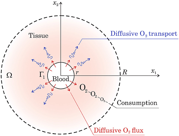
Figure 1. Projection of the model domain Ω onto the x₁Ox₂ plane.

To formalize the oxygen transport model, we introduce the functions M, f : ℝ → ℝ which are odd, increasing, and on the positive semiaxis defined as follows:

$M(t)=\frac{M_{0}t}{t+p_0},f(t)=at+\frac{b{t}^h}{t^h+c},h>1,t\ge 0,$

where M₀, p₀, a, b, and c are positive constants.

Using these notations, in the domain Ω, we consider the following oxygen transport model [6]:

$\begin{array}{ll}-\kappa \Delta p+M(p)=0,x\in \Omega ,& (1)\end{array}$

$\begin{array}{ll}p{|}_{{\Gamma }_1}=p_c(z)-\gamma q(z),z\in (0,L);{\partial }_{n}p{|}_{{\Gamma }_2}=0.& (2)\end{array}$

Here, p and p_c describe the partial pressure of oxygen (PO₂) in the tissue and capillary, respectively. The symbol Δ denotes the Laplace operator and ∂_n denotes the derivative in the direction of the outward normal n to the domain Ω. The function

$\begin{array}{l}q(z)=\kappa r{\displaystyle {\int }_0^{2\pi }}{\partial }_{n}p{|}_{{\Gamma }_1}d\theta \end{array}$

is interpreted as the diffusive oxygen flux entering the domain Ω from the capillary. The function p_c is determined from the equation

$\begin{array}{ll}-df(p_c(z))/dz=q(z)& (3)\end{array}$

and the initial condition

$\begin{array}{ll}{p}_c(0)=p_{+}.& (4)\end{array}$

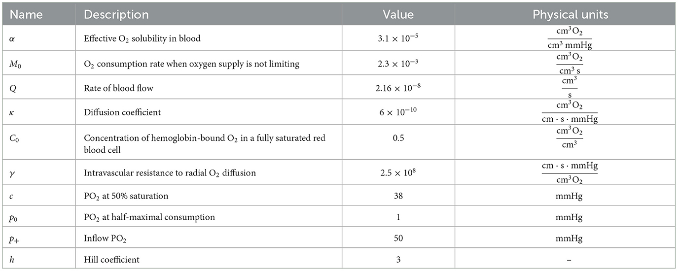
Here, θ is the polar angle on a circle. Positive parameters γ, κ, M₀, p₀, a, b, c, h, and p₊ are given. In more detail, γ is the intravascular resistance to the radial oxygen diffusion; a = αQ, where α is the effective solubility of oxygen in the blood, Q is the rate of blood flow; b = C₀H_DQ, where C₀ is the concentration of hemoglobin-bound oxygen in a fully saturated red blood cell, H_D is the discharge hematocrit; c is the partial oxygen pressure at 50% saturation; p₀ is the partial pressure of oxygen at half-maximal consumption; M₀ is the rate of oxygen consumption when oxygen supply is not limiting, h is the Hill coefficient. Values of the basic parameters of the model and their physical units are presented in Section 5.2 (Table 1).

TABLE 1

Table 1. Problem parameters [5, 6].

The non-linear term M(p) in Equation (1) is the rate of oxygen consumption in tissue presented above by the Michaelis–Menten relationship [6]. The function f(p_c) is the rate of convective oxygen transport along a vessel segment and q is the rate of diffusive oxygen efflux per unit vessel length. Accordingly, conservation of oxygen implies Equation (3) that describes the change in the partial pressure of oxygen in the capillary. The first equality in (2) with (3) and (4) describes the oxygen supply from the capillary.

Remark 1. In the case of a finite number of disjoint vessels, the boundary value problem is formulated in a similar way.

The system (1)–(4) can be considered as a boundary value problem in the domain Ω for the non-linear diffusion Equation (1). At the part of the boundary Γ₂, the Neumann boundary conditions are set, at the part of the boundary Γ₁ coinciding with the capillary wall, the tissue PO₂ depends on a solution of the non-linear Cauchy problem (3), (4) describing the oxygen transport in the blood. Thus, the equalities (2)–(4) represent non-linear boundary conditions for Equation (1).

Due to the specific non-linear boundary conditions (2)–(4), the considered problem is not a standard boundary value problem for an elliptic equation. Accordingly, some theoretical aspects such as the existence and uniqueness of a solution are open and of scientific interest.

3 Formalization of the problem

By L^s, 1 ≤ s ≤ ∞, we denote Lebesgue space of s- integrable functions, by H the Lebesgue space L²(Ω), and by H¹ the Sobolev space $W_2^1$. Let

$\begin{array}{l}W=\{w\in C^{\infty }(\overline{\Omega }):w{|}_{{\Gamma }_1}=w_b(z),\\ \text{i}.\text{e}.\text{ it depends only on }z,z\in (0,L)\},\end{array}$

and V be the closure of W with respect to the norm in H¹(Ω). Here and below, for the boundary values on Γ₁ of functions w from W and V, depending only on z, we use the notation w_b. Following these notations, for example, for p ∈ V, p|_Γ1 = p_b. By (f, v) we denote the inner product in H, by 〈f, v〉 the inner product in L²(0, L), and by ‖v‖ the norm in H, ‖v‖² = (v, v).

Let us define the operator T:L²(0, L) → H¹(0, L) such that ζ = Tη if

$\begin{array}{ll}\gamma \frac{df(\zeta (z))}{dz}+\zeta (z)=\eta (z),z\in (0,L),& (5)\end{array}$

and ζ(0) = p₊.

Lemma 1. The following estimate meaning the continuity of the operator T is valid:

$\begin{array}{ll}||T{\eta }_1-T{\eta }_2|{|}_{C\left[0,L\right]}\le \frac{2L^{1/2}}{\gamma a}||{\eta }_1-{\eta }_2|{|}_{L^2(0,L)}.& (6)\end{array}$

Proof. Let ζ_1,2 = Tη_1,2, y_1,2 = f(ζ_1,2), η = η₁ − η₂, y = y₁ − y₂. Then

$\begin{array}{ll}\gamma y^{\prime }(z)+g(y_1(z))-g(y_2(z))=\eta (z),z\in (0,L),y(0)=0.& (7)\end{array}$

Here, g is the inverse function to f, which is continuously differentiable, odd, and increasing. Taking into account that f′ ≥ a, we have 0 < g′ ≤ 1/a. Also, note that due to the monotonic increase of g, the inequality (g(y₁)−g(y₂))(y₁ − y₂) ≥ 0 holds.

Multiplying the equality (7) by y and integrating over (0, z), we obtain

$\begin{array}{c}{\displaystyle {\int }_0^z}\eta (s)y(s)ds=\gamma {\displaystyle {\int }_0^z}{y}^{\prime }(s)y(s)ds+\\ {\displaystyle {\int }_0^z}(g(y_1(s))-g(y_2(s)))(y_1(s)-y_2(s))ds\ge \frac{\gamma }{2}{y}^2(z).\hfill \end{array}$

On the other hand

${\displaystyle {\int }_0^z}\eta (s)y(s)ds\le ||\eta |{|}_{L^2(0,L)}||y|{|}_{L^2(0,L)}\le L^{1/2}||\eta |{|}_{L^2(0,L)}||y|{|}_{C\left[0,L\right]}.$

Therefore,

$\begin{array}{ll}\frac{\gamma }{2}||y|{|}_{C\left[0,L\right]}\le L^{1/2}||\eta |{|}_{L^2(0,L)}.& (8)\end{array}$

Further,

$\begin{array}{l}||{\zeta }_1-{\zeta }_2|{|}_{C\left[0,L\right]}=||g(y_1)-g(y_2)|{|}_{C\left[0,L\right]}\\ \le max|g^{\prime }|||y_1-y_2|{|}_{C\left[0,L\right]}\le \frac{1}{a}||y|{|}_{C\left[0,L\right]}.& (9)\end{array}$

As a result, the estimate (6) follows from inequalities (8) and (9).

Lemma 2.

$\begin{array}{ll}||T\eta |{|}_{L^2(0,L)}^2\le ||\eta |{|}_{L^2(0,L)}^2+2\gamma p_{+}f(p_{+}).& (10)\end{array}$

Proof. Let ζ = Tη. Multiplying the equality (5) in the sense of the inner product in L²(0, L) by ζ, we obtain

$\gamma \langle df(\zeta )/dz,\zeta \rangle +||\zeta |{|}_{L^2(0,L)}^2=\langle \eta ,\zeta \rangle .$

Note that

$\begin{array}{l}\langle df(\zeta )/dz,\zeta \rangle =\langle f^{\prime }(\zeta )d\zeta /dz,\zeta \rangle ={\displaystyle {\int }_0^L}{f}^{\prime }(\zeta )\frac{d\zeta }{dz}\zeta dz\\ =p_{-}f(p_{-})-p_{+}f(p_{-})-{\displaystyle {\int }_{p_{+}}^{p_{-}}}f(\zeta )d\zeta \ge -p_{+}f(p_{+}).\end{array}$

Here, p₋ = ζ(L). Therefore,

$\begin{array}{l}||\zeta |{|}_{L^2(0,L)}^2\le \langle \eta ,\zeta \rangle +\gamma p_{+}f(p_{+})\\ \le \frac{1}{2}||\zeta |{|}_{L^2(0,L)}^2+\frac{1}{2}||\eta |{|}_{L^2(0,L)}^2+\gamma p_{+}f(p_{+}).\end{array}$

This implies the estimate (10).

To derive a weak formulation of the boundary value problem (1) – (4), we multiply the Equation (1) by a test function v ∈ V and integrate by parts in Ω. As a result

$\begin{array}{ll}\kappa (\nabla p,\nabla v)+(M(p),v)-\kappa {\displaystyle {\int }_{{\Gamma }_1}}{\partial }_{n}p{|}_{{\Gamma }_1}{v}_{b}d\Gamma =0\forall v\in V.& (11)\end{array}$

Using (2), (3), and the definition of the operator T, we obtain the equality

$\begin{array}{l}q(z)=\frac{1}{\gamma }(T{p}_b(z)-p_b(z)).\end{array}$

Further, note that

$\begin{array}{l}\kappa {\displaystyle {\int }_{{\Gamma }_1}}{\partial }_{n}p{|}_{{\Gamma }_1}{v}_{b}d\Gamma =\\ {\displaystyle {\int }_0^L}\kappa r{\displaystyle {\int }_0^{2\pi }}{\partial }_{n}p(r,z,\theta )v_b(z)d\theta dz={\displaystyle {\int }_0^L}q(z)v_b(z)dz\\ =\frac{1}{\gamma }{\displaystyle {\int }_0^L}(T{p}_b(z)-p_b(z))v_b(z)dz=\frac{1}{\gamma }\langle T{p}_b-p_b,v_b\rangle .& (12)\end{array}$

Taking into account (11) and (12), we come to the following weak formulation of the boundary value problem (1)–(4).

Definition 1. Function p ∈ V is a weak solution of the boundary value problem (1)–(4) if

$\begin{array}{ll}\kappa (\nabla p,\nabla v)+(M(p),v)+\frac{1}{\gamma }\langle p_b-T{p}_b,v_b\rangle =0\forall v\in V.& (13)\end{array}$

4 Existence theorem of a weak solution

Let us define the Galerkin approximations p_m of a solution for the boundary value problem (1)–(4) and derive a priori estimates sufficient for the solvability of the problem. In the space V, we introduce a basis consisting of functions of the class W: w₁, w₂, …. Further, consider the following problem:

$\begin{array}{cc}\begin{array}{c}{p}_m={\displaystyle \sum _{j=1}^m}{\xi }_{j,m}{w}_j\in V_m,V_m:=\text{span}\left\{w_1,w_2,...,w_m\right\},\\ \kappa (\nabla p_m,\nabla w)+(M(p_m),w)+\frac{1}{\gamma }\langle p_{mb}-T{p}_{mb},w_b\rangle =0\forall w\in V_m.\end{array}& (14)\end{array}$

The equalities (14) give a system of non-linear equations with respect to the coefficients ξ_1,m, …, ξ_m,m of the Galerkin approximation p_m. To prove its solvability, it is convenient to use the following simple corollary from Brouwer's fixed point theorem [15, Ch. 2, Lemma 1.4].

Lemma 3. Let X be a finite-dimensional Hilbert space with an inner product [·, ·] and a norm [·], and F : X → X be a continuous mapping such that [F(ξ), ξ] > 0 for [ξ] = k. Then there is an element ξ^* ∈ X, [ξ^*] ≤ k, for which F(ξ^*) = 0.

Take as X the space V_m with the inner product

$\left[\phi ,\psi \right]=\left(\nabla \phi ,\nabla \psi \right)+\left({\displaystyle {\int }_{\Omega }}\phi dx\right)\left({\displaystyle {\int }_{\Omega }}\psi dx\right).$

We define a continuous mapping F as follows: ∀φ, ψ ∈ V_m

$\left[F\left(\phi \right),\psi \right]=\kappa \left(\nabla \phi ,\nabla \psi \right)+\left(M\left(\phi \right),\psi \right)+\frac{1}{\gamma }\langle {\phi }_b-T{\phi }_b,{\psi }_b\rangle .$

Then for φ ∈ V_m

$\begin{array}{l}\left[F\left(\phi \right),\phi \right]=\kappa ||\nabla \phi |{|}^2+\left(M\left(\phi \right),\phi \right)+\frac{1}{\gamma }\left(||{\phi }_b|{|}_{L^2\left(0,L\right)}^2-\langle T{\phi }_b,{\phi }_b\rangle \right)\\ \ge \kappa ||\nabla \phi |{|}^2+\left(M\left(\phi \right),\phi \right)+\frac{1}{2\gamma }\left(||{\phi }_b|{|}_{L^2\left(0,L\right)}^2-||T{\phi }_b|{|}_{L^2\left(0,L\right)}^2\right).\end{array}$

Therefore, by Lemma 2,

$\left[F\left(\phi \right),\phi \right]\ge \kappa ||\nabla \phi |{|}^2+\left(M\left(\phi \right),\phi \right)-p_{+}f\left(p_{+}\right).$

Taking into account the oddness of function M, we obtain that

$\begin{array}{l}\left(M\left(\phi \right),\phi \right)=M_0{\displaystyle {\int }_{\Omega }}\left(|\phi |-p_0+p_0^2/\left(|\phi |+p_0\right)\right)dx\\ >M_0{\displaystyle {\int }_{\Omega }}\left(|\phi |-p_0\right)dx\ge M_0\left|{\displaystyle {\int }_{\Omega }}\phi dx\right|-M_0{p}_0|\Omega |.\end{array}$

This allows us to get the following estimate:

$\begin{array}{l}\left[F\left(\phi \right),\phi \right]>\kappa ||\nabla \phi |{|}^2+M_0\left|{\displaystyle {\int }_{\Omega }}\phi dx\right|-C_1,\\ C_1=p_{+}f\left(p_{+}\right)+M_0{p}_0|\Omega |.\end{array}$

From the last inequality, it follows that

$\left[F\left(\phi \right),\phi \right]>0\text{for }||\nabla \phi |{|}^2+|{\displaystyle {\int }_{\Omega }}\phi dx{|}^2=k^2$

if k is large enough, for example, $k^2>2\mathrm{\text{max}}\left\{C_1/\kappa ,C_1^2/M_0^2\right\}.$ Indeed, in the case

$||\nabla \phi |{|}^2+|{\displaystyle {\int }_{\Omega }}\phi dx{|}^2=k^2,$

either ‖∇φ‖² ≥ k²/2 and then $\left[F\left(\phi \right),\phi \right]>\kappa k^2/2-C_1$, or

$|{\displaystyle {\int }_{\Omega }}\phi dx{|}^2\ge k^2/2$

and then $\left[F\left(\phi \right),\phi \right]>M_{0}k/\sqrt{2}-C_1$. Therefore, if $k^2>2max\left\{C_1/\kappa ,C_1^2/M_0^2\right\}$, then [F(φ), φ] > 0.

By virtue of Lemma 3, there exists a solution p_m of the problem (14) such that

$0=\left[F\left(p_m\right),p_m\right]>\kappa ||\nabla p_m|{|}^2+M_0\left|{\displaystyle {\int }_{\Omega }}{p}_{m}dx\right|-C_1.$

Therefore, for the Galerkin approximations, the following estimate is valid:

$\begin{array}{ll}{\left[p_m\right]}^2=||\nabla p_m|{|}^2+|{\displaystyle {\int }_{\Omega }}{p}_{m}dx{|}^2\le C_2,& (15)\end{array}$

where C₂ does not depend on m. As C₂ we can take C₁/min{κ, M₀}. Since the norm [·] in (15) is equivalent to the norm of H¹(Ω) [16, Lemma 7.1], passing to a subsequence, we conclude that there exists p ∈ V such that

$\begin{array}{l}{p}_m\to p\text{ weakly in }V,\text{ strongly in }H,\\ p_m{|}_{{\Gamma }_1}\to p{|}_{{\Gamma }_1}\text{ strongly in }{L}^2({\Gamma }_1).& (16)\end{array}$

Taking into account the boundedness of the derivative of the function M and the continuity of the operator T, the results on the convergence (16) are sufficient to justify the passage to the limit in Equation (14). Indeed,

$|(M(p_m)-M(p),w_j)|\le \frac{M_0}{p_0}max|w_j|{\displaystyle {\int }_{\Omega }}|p_m-p|dx\to 0,$

and taking into account (6),

$||T{p}_{mb}-T{p}_b|{|}_{C\left[0,L\right]}\le \frac{2L^{1/2}}{\gamma a}||p_{mb}-p_b|{|}_{L^2(0,L)}\to 0.$

Moreover, (∇p_m, ∇w_j) → (∇p, ∇w_j). Setting w = w_j, j < m, in Equation (14) and passing to the limit as m → +∞, we conclude that Equation (13) is valid for v = w₁, w₂, …, as well as for any function v that is a linear combination of w₁, w₂, …. Because these combinations are dense in V, then we obtain Equation (13).

Theorem 1. There exists a weak solution p ∈ V of the problem (1)–(4) such that

$\kappa ||\nabla p|{|}^2+M_0\left|{\displaystyle {\int }_{\Omega }}pdx\right|\le p_{+}f\left(p_{+}\right)+M_0{p}_0|\Omega |.$

5 Numerical experiments

5.1 Iterative algorithm

To find a solution to the boundary value problem (1)–(4), we build an iterative algorithm that yields a functional series ${\{p^{(m)}\}}_{m=0}^{\infty }$ such that p^(m) → p as m → ∞. At m + 1 step of the iterative algorithm, we find the approximation p^{(m + 1)} as a solution of the following boundary value problem:

$\begin{array}{ll}-\kappa \Delta p^{(m+1)}+\frac{M_0{p}^{(m+1)}}{p^{(m)}+p_0}=0,x\in \Omega ,& (17)\end{array}$

$\begin{array}{ll}{p}^{(m+1)}{|}_{{\Gamma }_1}=p_c^{(m)}(z)-\gamma q^{(m)}(z),z\in (0,L);{\partial }_n{p}^{(m+1)}{|}_{{\Gamma }_2}=0,& (18)\end{array}$

where

$\begin{array}{ll}{q}^{(m)}(z)=\kappa r{\displaystyle {\int }_0^{2\pi }}{\partial }_n{p}^{(m)}{|}_{{\Gamma }_1}d\theta ,z\in (0,L),& (19)\end{array}$

$\begin{array}{ll}-df(p_c^{(m)}(z))/dz=q^{(m)}(z),z\in (0,L);p_c^{(m)}(0)=p_{+}.& (20)\end{array}$

Here, p^(m) is an approximation obtained at the previous step of the iterative algorithm.

Computational domain in cylindrical coordinates, taking into account axial symmetry, is shown in Figure 2. To implement each step of the iterative algorithm, the FreeFEM++ software is utilized [17]. In more detail, the description of the iterative algorithm is below (see Algorithm 1).

FIGURE 2

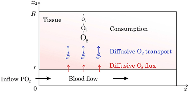
Figure 2. Computational domain in cylindrical coordinates, taking into account the axial symmetry.

ALGORITHM 1

Algorithm 1. Iterative algorithm.

5.2 Risk factors of hypoxia in preterm infants

The problem parameters used in [5, 6] to simulate the oxygen transport in the brain are set to conduct numerical experiments (see Table 1). Additionally, we set r = 3μm, R = 30μm, and L = 60μm.

Consider risk factors for hypoxia in preterm infants. The first is a low hematocrit. An analytical approximation presented in [1] gives the systemic hematocrit value of 0.46 for term infants of 40 gestational weeks (GW) on the 7th day after birth and 0.36 for preterm infants of 25 gestational weeks on the 7th day after birth. Further, on the basis of data from different sources analyzed in [18], the tube hematocrit in capillaries is 26–42% of the systemic hematocrit. By setting the reduction factor for the systematic hematocrit as 0.34, we get the capillary hematocrit equal to 0.16 for term (40 GW) and 0.12 for preterm (25 GW) infants. To obtain the discharge hematocrit in capillaries with a given diameter, an analytical approximation presented in [19] can be applied. As a result, the discharge hematocrit in capillaries with a diameter of 6 μm is evaluated as 0.22 for term (40 GW) and 0.17 for preterm (25 GW) infants.

For the discharge hematocrit equal to 0.22, the distribution of the tissue PO₂ in the plane zOx₂ is shown in Figure 3. Here, the bottom side of the computational domain corresponds to the capillary wall. The drop in the discharge hematocrit from 0.22 to 0.17, i.e., by 23%, leads to a decrease in the tissue PO₂. The corresponding relative reduction of the tissue PO₂ is shown in Figure 4. Due to the decrease in the discharge hematocrit, the tissue PO₂ drops up to 13%.

FIGURE 3

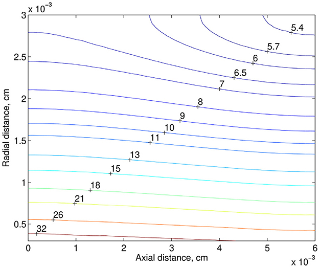
Figure 3. PO₂ distribution in the tissue (mmHg). The bottom side of the computational domain corresponds to the capillary wall.

FIGURE 4

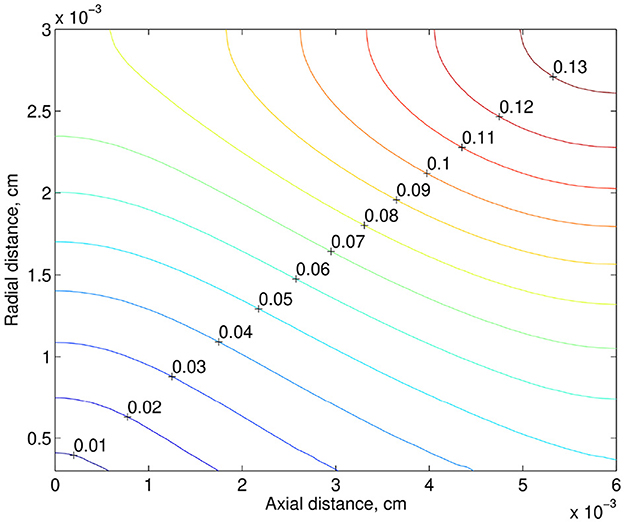
Figure 4. Relative reducing the tissue PO₂, when the discharge hematocrit drops from 0.22 to 0.17.

Another risk factor of hypoxia is a low rate of blood flow. Note that some medical data show that preterm infants have a lower rate of CBF compared to measurements in term infants [2, 3]. For example, on the base of data reported in [2], the mean CBF in preterm infants was 4.9–23 ml / l00g / min. At the same time the range of mean CBF in term infants was 9.0–73 ml/100 g/min. Also, note that for ventilated preterm infants 30% decrease in CBF is observed compared to healthy preterm infants [20]. Thus, the reduction in the blood flow rate in preterm infants can be quite significant. In the numerical simulation, we consider the case of its 40% drop. In the next numerical experiment in addition to the drop in the discharge hematocrit (from 0.22 to 0.17), the rate of blood flow decreased by 40%. The relative reduction of the tissue PO₂, when the discharge hematocrit drops from 0.22 to 0.17 and the rate of blood flow drops from 2.16 × 10⁻⁸ to 1.30 × 10⁻⁸cm³/s, is shown in Figure 5. Due to the decrease in the discharge hematocrit and the rate of blood flow, the tissue PO₂ drops up to 43%.

FIGURE 5

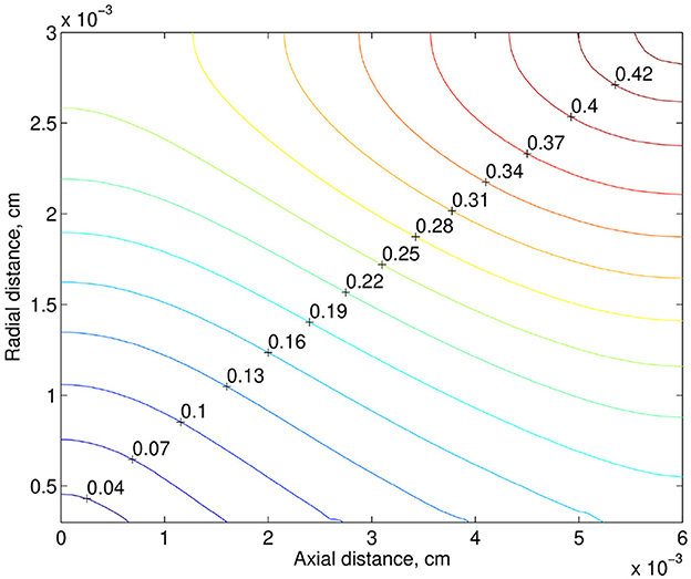
Figure 5. Relative reducing the tissue PO₂, when the discharge hematocrit drops by 23% from 0.22 to 0.17 and the rate of blood flow drops by 40% from 2.16 × 10⁻⁸ to 1.30 × 10⁻⁸cm³/s.

Note that the results obtained are consistent with numerical simulations based on a similar model proposed in [10] and developed in subsequent work [11], but unlike the present work, intravascular oxygen transport is modeled there in more detail and requires taking into account the spatial distribution of red blood cells. In [11], the authors showed that a decrease in the linear density of RBCs and their velocity leads to a decrease in the tissue PO₂. This is in agreement with the results presented in the current article since a decrease in the linear density of RBCs and their velocity means a decrease in hematocrit level and blood flow rate.

6 Conclusion

The numerical modeling of oxygen transport in the simplified domain makes it possible to quantify the influence of various factors on the partial pressure of oxygen at different distances from the capillary. Low levels of hematocrit and cerebral blood flow, often observed in preterm infants, are risk factors for cerebral tissue hypoxia. In the numerical simulation performed, with a typical decrease in hematocrit and cerebral blood flow rate in premature infants by 23 and 40%, respectively, the decrease in the tissue PO₂ is about 43% or more in some areas of the model domain. As further calculations showed, with a decrease in the blood flow rate by 50 and 60%, which is possible according to the medical data presented in [2], the tissue PO₂ drops up to 53 and 66%, respectively.

Based on the numerical simulations carried out, it can be concluded that levels of the hematocrit and cerebral blood flow rate have an important effect on the tissue PO₂ in the brain, their critical decrease leading to hypoxia can be estimated on the basis of the simplified model of oxygen transport and medical data. This will allow, in the event of a critical decrease in the hematocrit and rate of blood flow, to carry out therapeutic measures in advance to avoid possible irreversible consequences in the brain tissue.

Data availability statement

The original contributions presented in the study are included in the article/supplementary material, further inquiries can be directed to the corresponding author.

Author contributions

AK: Conceptualization, Formal analysis, Investigation, Methodology, Software, Validation, Visualization, Writing—original draft, Writing—review & editing. AC: Conceptualization, Formal analysis, Investigation, Methodology, Validation, Writing—original draft, Writing—review & editing. RL: Conceptualization, Funding acquisition, Project administration, Supervision, Writing—original draft, Writing—review & editing.

Funding

The author(s) declare financial support was received for the research, authorship, and/or publication of this article. This research was funded by the Klaus Tschira Foundation (grant number 00.302.2016), Buhl-Strohmaier Foundation, and Würth Foundation.

Acknowledgments

The authors kindly thank the TUM Open Access Publishing Fund, Klaus Tschira Foundation, Buhl-Strohmaier Foundation, and Würth Foundation.

Conflict of interest

The authors declare that the research was conducted in the absence of any commercial or financial relationships that could be construed as a potential conflict of interest.

Publisher's note

All claims expressed in this article are solely those of the authors and do not necessarily represent those of their affiliated organizations, or those of the publisher, the editors and the reviewers. Any product that may be evaluated in this article, or claim that may be made by its manufacturer, is not guaranteed or endorsed by the publisher.

References

1. Scholkmann F, Ostojic D, Isler H, Bassler D, Wolf M, Karen T. Reference ranges for hemoglobin and hematocrit levels in neonates as a function of gestational age (22–42 weeks) and postnatal age (0–29 days): mathematical modeling. Children. (2019) 6:38. doi: 10.3390/children6030038

PubMed Abstract | CrossRef Full Text | Google Scholar

2. Altman DI, Powers WJ, Perlman JM, Herscovitch P, Volpe SL, Volpe JJ. Cerebral blood flow requirement for brain viability in newborn infants is lower than in adults. Ann Neurol. (1988) 24:218–26. doi: 10.1002/ana.410240208

PubMed Abstract | CrossRef Full Text | Google Scholar

3. Brew N, Walker D, Wong FY. Cerebral vascular regulation and brain injury in preterm infants. Am J Physiol Regul Integr Comp Physiol. (2014) 306:R773–86. doi: 10.1152/ajpregu.00487.2013

PubMed Abstract | CrossRef Full Text | Google Scholar

4. Pittman RN. Regulation of Tissue Oxygenation. San Rafael, CA: Morgan and Claypool Life Sciences (2011).

Google Scholar

5. Secomb TW, Hsu R, Beamer NB, Coull BM. Theoretical simulation of oxygen transport to brain by networks of microvessels: effects of oxygen supply and demand on tissue hypoxia. Microcirculation. (2000) 7:237–47. doi: 10.1111/j.1549-8719.2000.tb00124.x

PubMed Abstract | CrossRef Full Text | Google Scholar

6. Secomb TW, Hsu R, Park EYH, Dewhirst MW. Green's function methods for analysis of oxygen delivery to tissue by microvascular networks. Ann Biomed Eng. (2004) 32:1519–29. doi: 10.1114/B:ABME.0000049036.08817.44

PubMed Abstract | CrossRef Full Text | Google Scholar

7. Lu Y, Hu D, Ying W. A fast numerical method for oxygen supply in tissue with complex blood vessel network. PLoS ONE. (2021) 16:1–25. doi: 10.1371/journal.pone.0247641

PubMed Abstract | CrossRef Full Text | Google Scholar

8. Kovtanyuk AE, Chebotarev AY, Botkin ND, Turova VL, Sidorenko IN, Lampe R. Continuum model of oxygen transport in brain. J Math Anal Appl. (2019) 474:1352–63. doi: 10.1016/j.jmaa.2019.02.020

CrossRef Full Text | Google Scholar

9. Kovtanyuk AE, Chebotarev AY, Botkin ND, Turova VL, Sidorenko IN, Lampe R. Nonstationary model of oxygen transport in brain tissue. Comput Math Methods Med. (2020) 2020:4861654. doi: 10.1155/2020/4861654

PubMed Abstract | CrossRef Full Text | Google Scholar

10. Lücker A, Weber B, Jenny P. A dynamic model of oxygen transport from capillaries to tissue with moving red blood cells. Am J Physiol Heart Circ Physiol. (2015) 308:H206–16. doi: 10.1152/ajpheart.00447.2014

PubMed Abstract | CrossRef Full Text | Google Scholar

11. Lücker A, Secomb TW, Weber B, Jenny P. The relative influence of hematocrit and red blood cell velocity on oxygen transport from capillaries to tissue. Microcirculation. (2017) 24:e12337. doi: 10.1111/micc.12337

PubMed Abstract | CrossRef Full Text | Google Scholar

12. Lücker A, Secomb TW, Weber B, Jenny P. The relation between capillary transit times and hemoglobin saturation heterogeneity. part 1: theoretical models. Front Physiol. (2018) 9:420. doi: 10.3389/fphys.2018.00420

PubMed Abstract | CrossRef Full Text | Google Scholar

13. Valabrègue R, Aubert A, Burger J, Bittoun J, Costalat R. Relation between cerebral blood flow and metabolism explained by a model of oxygen exchange. J Cerebr Blood Flow Metab. (2003) 23:536–45. doi: 10.1097/01.WCB.0000055178.31872.38

PubMed Abstract | CrossRef Full Text | Google Scholar

14. Piechnik SK, Chiarelli PA, Jezzard P. Modelling vascular reactivity to investigate the basis of the relationship between cerebral blood volume and flow under CO2 manipulation. Neuroimage. (2008) 39:107–18. doi: 10.1016/j.neuroimage.2007.08.022

PubMed Abstract | CrossRef Full Text | Google Scholar

15. Temam R. Navier-Stokes Equations: Theory and Numerical Analysis. Providence, RI: AMS Chelsea Publishing (1984).

Google Scholar

16. Duvant G, Lions JL. Inequalities in Mechanics and Physics. Berlin; Heidelberg; New York, NY: Springer Science and Business Media (2012).

Google Scholar

17. Hecht F. New development in freefem++. J Numer Math. (2012) 20:251–65. doi: 10.1515/jnum-2012-0013

CrossRef Full Text | Google Scholar

18. Goldsmith HL, Cokelet GR, Gaehtgens P. Robin Fahraeus: evolution of his concepts in cardiovascular physiology. Am J Physiol Heart Circ Physiol. (1989) 257:H1005–15. doi: 10.1152/ajpheart.1989.257.3.H1005

PubMed Abstract | CrossRef Full Text | Google Scholar

19. Pries AR, Neuhaus D, Gaehtgens P. Blood viscosity in tube flow: dependence on diameter and hematocrit. Am J Physiol Heart Circ Physiol. (1992) 263:H1770–8. doi: 10.1152/ajpheart.1992.263.6.H1770

PubMed Abstract | CrossRef Full Text | Google Scholar

20. Eiby YA, Lingwood BE, Wright IMR. Plasma leak from the circulation contributes to poor outcomes for preterm infants: a working hypothesis. Front Neurol. (2021) 12:636740. doi: 10.3389/fneur.2021.636740

PubMed Abstract | CrossRef Full Text | Google Scholar