Geometry of deviation measures for triangular distributions

Triangular distributions are widely used in many applications with limited sample data, business simulations, and project management. As with other distributions, a standard way to measure deviations is to compute the standard deviation. However, the standard deviation is sensitive to outliers. In this paper, we consider and compare other deviation metrics, namely the mean absolute deviation from the mean, the median, and the quantile-based deviation. We show the simple geometric interpretations for these deviation measures and how to construct them using a compass and a straightedge. The explicit formula of mean absolute deviation from the median for triangular distribution is derived in this paper for the first time. It has a simple geometric interpretation. It is the least volatile and is always better than the standard or mean absolute deviation from the mean. Although greater than the quantile deviation, it is easier to compute with limited sample data. We present a new procedure to estimate the parameters of this distribution in terms of this deviation. This procedure is computationally simple and may be superior to other methods when dealing with limited sample data, as is often the case with triangle distributions.

1 Introduction

Triangular distributions Tr(a, b, c) are a three-parameter distribution with a minimum value a, a maximum value b, and a most likely (mode) value c [1]. Unlike the uniform distribution, triangle distributions include the most likely value c in addition to the minimum and maximum values and allow for incorporating skewness and asymmetry. These distributions are widely used in business simulations, risk and project management, Monte-Carlo simulations, and other areas, especially when dealing with limited sample data [2–4] (for a historical review, see [1]).

As noted in [5], several authors [1, 6] have suggested using this distribution instead of the beta distribution since for beta distribution, there are difficulties in the maximum likelihood estimation of parameters and their interpretation. Johnson [6] and Johnson and Kotz [7] dealt with neglected applications of this distribution as an alternative to the beta distribution, which suffers from difficulties in its maximum likelihood parameter estimation. Triangular distributions are recommended when the underlying distribution is unknown, but a minimal value, some maximal value, and a most likely value are available [1].

This paper focuses on computing and comparing the deviation measures for such distributions, both geometrically and algebraically. Historically, the most widely used deviation measure has been the standard deviation [8]. In computing this metric, we square the distances from the mean. This usage of the L₂ norm is convenient in differentiation, optimization, and estimation [9]. However, this metric has some disadvantages, such as sensitivity to outliers. An alternative is to use the mean absolute deviation (the L₁-norm) and measure deviations (MAD) from a central point such as mean μ [denoted by H(μ)] or median M [denoted in this paper by H(M)]. On the other hand, using L₁ metric allows one to introduce performance metrics that do not require the computation of higher-order moments (e.g. [10]).

One of the contributions of this paper is an explicit formula for H(M), the mean absolute deviation about the median. The formula has a simple, intuitive, and geometric interpretation. To our knowledge, this is the first paper deriving an explicit formula for H(M) for the triangular distribution. For this distribution, deviation measures such as standard deviation, mean absolute deviation (about median), and quartile deviation have simple geometric interpretations and can all be constructed by a ruler and compass. The mean absolute deviation about the median H(M) is the least volatile and is always lower than the standard deviation or the MAD deviation about the mean. Although it is higher than the quartile deviation, it is more practical. We often have very limited data for triangular distributions, and accurate quartile estimates are problematic. Using H(M), we present a new non-iterative procedure to estimate the parameters of this distribution. This procedure is very simple computationally and is more robust than direct estimation based on the sample mean.

This paper is organized as follows. In Section 2, we introduce triangular distributions, compare mean and median, and present geometric interpretations for mean, median, and standard deviation. In Section 3 we derive a general expression for computing mean absolute deviations for triangular distributions. From this expression, we compute the mean absolute deviations H(μ) and H(M) about mean and median and provide a simple geometric interpretation for these measures. In Section 4, we introduce a new estimation procedure based on mean absolute deviation H(M) and illustrate it with a numerical example. In Section 5, we compare the exact values of tail probabilities with some estimates using deviations. In Section 6, we derive the formula for the quartile deviation. Finally, in Section 7 we present a detailed comparison of deviation measures.

2 Triangular distributions

We start with definitions and notations. Suppose X is distributed according to triangular distribution on the range [a, b] and mode parameter c ∈ [a, b]. We will write this as X ~ Tr(a, b, c). The density function f(x) and the cumulative distribution function F(x) is given given by

$\begin{array}{ll}f(x)=\{\begin{array}{l}\frac{2(x-a)}{(b-a)(c-a)}\hfill \\ \frac{2(b-x)}{(b-a)(b-c)}\hfill \end{array}F(x)=\{\begin{array}{ll}\frac{{(x-a)}^2}{(b-a)(c-a)}\hfill & \text{for }a\le x\le c,\hfill \\ 1-\frac{{(b-x)}^2}{(b-a)(b-c)}\hfill & \text{for }c<x\le b\hfill \end{array}& (1)\end{array}$

The mean μ and standard deviation σ are:

$\begin{array}{ll}\mu =(a+b+c)/3\text{ and }\sigma =\sqrt{a^2+b^2+c^2-ab-ac-bc}/3\sqrt{2}& (2)\end{array}$

Let F⁻¹(·) be the quantile function defined by F⁻¹(t) = inf{x:F(x) ≥ t} with t ∈ [0, 1]. From the definition of the cumulative distribution function, we find

$\begin{array}{ll}x=F^{-1}(t)=\{\begin{array}{ll}a+\sqrt{t(b-a)(c-a)}\hfill & a\le x\le c\hfill \\ b-\sqrt{(1-t)(b-a)(b-c)}\hfill & c<x\le b\hfill \end{array}& (3)\end{array}$

Therefore, for the median M = F⁻¹(1/2) we have

$\begin{array}{ll}\{\begin{array}{ll}(b-M)=\frac{\sqrt{2}}{2}\sqrt{(b-a)(b-c)}\hfill & c\le (a+b)/2\hfill \\ (M-a)=\frac{\sqrt{2}}{2}\sqrt{(b-a)(c-a)}\hfill & c\ge (a+b)/2\hfill \end{array}\hfill & (4)\end{array}$

We will find it convenient to consider a standard (“normalized”) variable under min-max transformation X ↦ (X − a)/(b − a). Then, X has a triangular distribution with a = 0, b = 1 and a ≤ c ≤ b. For this standard X, the mean μ = (1 + c)/3, standard deviation $\sqrt{1+c^2-c}/3\sqrt{2}$ whereas the median $M=1-\sqrt{2(1-c)}/2$ for c ≤ 1/2 and $M=\sqrt{c/2}\text{ for }1/2\le c\le 1$.

In Table 1, we compute mean, median and standard deviation for standard triangle distribution (a = 0, b = 1) for c = 0, c = 1/4, c = 1/2, c = 3/4, and c = 1.

TABLE 1

Table 1. Mean, median, and standard deviation.

The case c = 0 corresponds to the distribution X = |U₁−U₂| of the absolute difference between two independent random variables U₁ and U₂ with standard uniform distribution. By contrast, the symmetric case c = 1/2 corresponds to the distribution X = (U₁ + U₂)/2 of the mean of the sum of two standard uniform variables U₁ and U₂.

The mean μ, the median M, the standard deviation σ, and other deviation measures discussed in this paper have simple geometric interpretations and can be constructed using a straightedge and compass. For their constructions, we will assume that we know how to do the following:

1. construct a segment of unit length

2. copy segments and angles

3. construct (l₁ + l₂) and (l₁ − l₂) from segments of lengths l₁ and l₂

4. divide length l into 2 (bisection) equal or 3 equal parts (trisection)

5. construct 30°/60° and 45°/45° right triangles with a side (e.g., hypotenuse) of length l. This allows computing $l\sqrt{2}$, $l/\sqrt{2}$, $l\sqrt{3}$, and $l/\sqrt{3}$

6. construct a right triangle with sides l₁ and l₂

7. compute the geometric mean $\sqrt{l_1{l}_2}$ of two segments with lengths l₁ and l₂. This construction is illustrated in Figure 1.

FIGURE 1

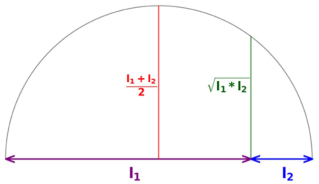
Figure 1. Geometric interpretation for geometric mean.

We can now discuss the geometric construction and interpretation of some measures for this distribution.

2.1 Geometric construction and interpretation of the mean

To construct μ, it will be sufficient to construct (μ − a). From Equation (2) we have (μ − a) = (c − a)/3 + (b − a)/3. This gives us the following construction for (μ − a):

1. trisect (b − a) to compute l₁ = (b − a)/3

2. trisect (c − a) to compute l₂ = (c − a)/3

3. compute (μ − a) = l₁+l₂

The mean μ has the following interesting interpretation: Consider a triangle with vertices (x₁, y₁), (x₂, y₂), and (x₃, y₃). Consider the centroid K of such a triangle: the point at which the three medians of the triangle intersect as shown in Figure 2. This centroid is the point with coordinates (x₁ + x₂ + x₃)/3, (y₁ + y₂ + y₃)/3. To construct this point, we bisect the sides of the triangle and draw lines from vertices to the midpoints of the opposite sides. These three lines meet at the single point K. By the centroid theorem, the point K is 2/3 of the distance from the vertex to the midpoint of the sides. If we use the geometric interpretation of the density as a triangle with vertices (a, 0), (b, 0), and (c, 2/(b − a)), then the x-coordinate of its centroid is the mean μ.

FIGURE 2

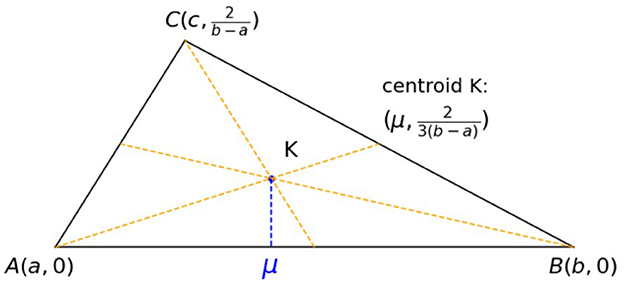
Figure 2. Mean and the triangle centroid.

Next, we establish the relationship between the mean μ and the midpoint (a + b)/2. If c ≤ (a + b)/2, then 3c ≤ (a + b + c) or c ≤ μ. On the other hand, μ = (a + b + c)/3 ≤ ((a + b) + (a + b)/2)/3 = (a + b)/2 and thus, c ≤ μ ≤ (a + b)/2. Therefore,

$\begin{array}{ll}0\le c\le (a+b)/2\Rightarrow \mu \ge c\text{\hspace{1em}and\hspace{1em}}(a+b)/2\le c\le b\Rightarrow \mu \le c& (5)\end{array}$

2.2 Geometric construction and interpretation of the median

The median M has a different geometric interpretation. We consider the case c ≤ (a + b)/2. To construct M, it will be sufficient to construct (M − a). We proceed as follows:

1. compute the geometric mean $l_1=\sqrt{(b-a)(b-c)}$

2. (any other) side of this triangle has the length $(M-a)=l_1\sqrt{2}/2$

This is illustrated in Figure 3.

FIGURE 3

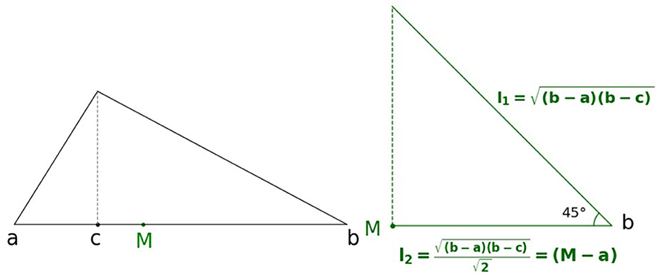
Figure 3. Geometric interpretation of median when c ≤ (a + b)/2.

For the case c ≥ (a + b)/2, we construct (b − M) by similar steps:

1. compute the geometric mean $l_1=\sqrt{(b-a)(c-a)}$

2. (any other) side of this triangle has a length $(b-M)=l_1\sqrt{2}/2$

Next, we establish the relationship between the median M and the midpoint (a + b)/2. There are two cases to consider:

• Case 1: c ≤ (a + b)/2. In this case (b − a) ≤ 2(b − c) and from Equation (4) and we have

$\begin{array}{l}M=b-\sqrt{(b-a)(b-c)}/\sqrt{2}\ge b-(b-c)=c\end{array}$

• Case 2: c ≥ (a + b)/2. In this case, (b − a) ≤ 2(c − a) and we have

$\begin{array}{l}M=a+\sqrt{(b-a)(c-a)}/\sqrt{2}\le a+(c-a)=c\end{array}$

Therefore, we obtain the following relationship:

$\begin{array}{ll}a\le c\le (a+b)/2\Rightarrow M\ge c\text{\hspace{1em}and\hspace{1em}}(a+b)/2\le c\le b\Rightarrow M\le c& (6)\end{array}$

The case c ≤ (a + b)/2 is illustrated in Figure 4.

FIGURE 4

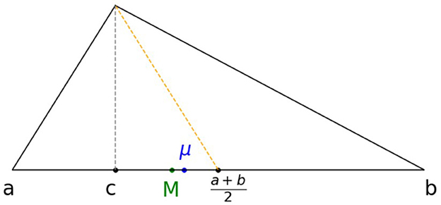
Figure 4. Mean and median for c ≤ (a + b)/2.

2.3 Relationship of mean and median

We show that for a ≤ c ≤ (a + b)/2 we have c ≤ M ≤ μ and for (a + b)/2 ≤ c ≤ b we have μ ≤ M ≤ c. There are two cases to consider:

• Case 1: a ≤ c ≤ (a + b)/2. In this case, (b − a)(b − c) ≥ (b − a)²/2 and from the Equation (4)

$\begin{array}{c}M=\frac{b^2-\frac{1}{2}(b-a)(b-c)}{b+\frac{\sqrt{2}}{2}\sqrt{(b-a)(b-c)}}\le \frac{1}{2}·\frac{(b^2+ab+bc-ac)}{b+\frac{1}{2}(b-a)}\\ \le \frac{(a+b+c)}{3}=\mu & (7)\end{array}$

• Case 2: (a + b)/2 ≤ c ≤ b. If we consider the distribution Y = (a + b)−X then by symmetry from the above Equation (7) we have μ ≤ M ≤ c.

Combining these results with Equation (6) we obtain the following relationship between the mean μ, the median M and the mode c:

$\begin{array}{ll}\begin{array}{cc}a\le c\le (a+b)/2& \Rightarrow a\le M\le \mu \le c\\ (a+b)/2\le c\le b& \Rightarrow c\le \mu \le M\le b\end{array}& (8)\end{array}$

2.4 Geometric construction and interpretation of the standard deviation

To derive a geometric interpretation for σ, we can re-write the expression for σ in Equation (2) as follows

$\begin{array}{ll}\sigma =\frac{1}{3}·\frac{1}{\sqrt{2}}\sqrt{{(b-a)}^2-(c-a)(b-c)}& (9)\end{array}$

From this equation, we immediately obtain $\sigma \le \sqrt{2}(b-a)/6$. For the case c = a or c = b, we have the equality $\sigma =\sqrt{2}(b-a)/6$.

The above Equation (9) suggests the following geometric construction and interpretation for the standard deviation σ are shown in Figure 5.

1. compute the geometric mean $l_2=\sqrt{(c-a)(b-c)}$

2. construct the right triangle T with hypotenuse (b − a) as side l₁.

3. compute the length $l_3=\sqrt{{(b-a)}^2-l_1^2}$ of the other side of T

4. compute the length $l_4=l_3/\sqrt{2}$

5. trisect l₃ to compute σ = l₄/3

FIGURE 5

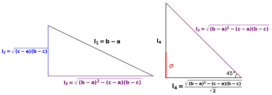
Figure 5. Geometric interpretation for standard deviation.

3 Mean absolute deviation

We start with preliminary definitions. Consider a real-valued random variable X with density f(x), finite mean and cumulative distribution function F(x). We use M, μ = E(X) and σ to denote median, mean and standard deviation of X respectively. For any p, we define the mean absolute deviation of X from p as

$\begin{array}{ll}H(p)=E(|X-p|)={\displaystyle {\int }_X}|x-p|f(x)dx& (10)\end{array}$

It can be interpreted as the average distance of values of X to the point p. If p = μ, then H(μ) is the mean absolute deviation from the mean μ. If we take p = M, then H(M) is the mean absolute deviation from the median. Both are denoted as MAD (mean absolute deviation) in the statistical literature, leading to some confusion [9].

It can be shown (details are presented in the Appendix) that for any distribution σ ≥ H(μ) ≥ H(M). Of the three metrics to measure deviations, namely H(M), H(μ), and σ, the MAD metric H(M) has the lowest value. In the computation of σ, we square distances (from the mean), and this inflates the impact of outliers. By contrast, we use these distances directly to compute mean absolute deviations. In addition, it is often easier to interpret mean absolute deviations than the standard deviation.

We illustrate this with a simple example. Suppose X is distributed according to a uniform distribution in [a, b]. Its density f(x) = 1/(b − a) and its cumulative distribution function F(x) = (x − a)/(b − a). For this distribution, μ = M = (a + b)/2, and $\sigma =\sqrt{3}(b-a)/6$. Since this distribution is symmetric, the MAD deviations H(M) = H(μ) and are easily computed H(M) = (b − a)/4 (e.g. [10]). The MAD value H(M) = (b − a)/4 is easy to interpret: it represents the average distance of X from its median M = (a + b)/2. However, it is more difficult to find an easy interpretation for standard deviation $\sigma =\sqrt{3}(b-a)/6$.

In the Appendix, we provide computational details on computing H(μ) and H(M). These are summarized below:

For triangular distribution, the mean absolute deviation from the mean H(μ) is

$\begin{array}{ll}H(\mu )=\{\begin{array}{ll}\frac{2{(a+c-2b)}^3}{81(a-b)(b-c)}\hfill & a\le c\le (a+b)/2\hfill \\ \frac{2{(b+c-2a)}^3}{81(a-b)(a-c)}\hfill & (a+b)/2\le c\le b\hfill \end{array}& (11)\end{array}$

For the standard triangular distribution with a = 0, b = 1 this simplifies to:

$\begin{array}{ll}H(\mu )=\{\begin{array}{ll}\frac{2}{3(1-c)}{\left(\frac{2-c}{3}\right)}^3\hfill & 0\le c\le 1/2\hfill \\ \frac{2}{3c}{\left(\frac{1+c}{3}\right)}^3\hfill & 1/2\le c\le 1\hfill \end{array}& (12)\end{array}$

For the mean absolute deviation H(M) from the median we obtain

$\begin{array}{ll}H(M)=\{\begin{array}{ll}\frac{(b-a)+(b-c)-\sqrt{2(b-a)(b-c)}}{3}\hfill & a\le c\le (a+b)/2\hfill \\ \frac{(b-a)+(c-a)-\sqrt{2(b-a)(c-a)}}{3}\hfill & (a+b)/2\le c\le b\hfill \end{array}& (13)\end{array}$

For the standard triangular distribution with a = 0, b = 1, this simplifies to

$\begin{array}{ll}H(M)=\{\begin{array}{ll}\frac{1}{3}(2-c-\sqrt{2(1-c)})\hfill & 0\le c\le 1/2\hfill \\ \frac{1}{3}(1+c-\sqrt{2c})\hfill & 1/2\le c\le 1\hfill \end{array}& (14)\end{array}$

3.1 Geometric construction and interpretation of MAD

The Equation (13) gives us the following procedure for the geometric construction of H(M). We consider two cases:

• Case 1: a ≤ c ≤ (a + b)/2. We construct H(M) as follows:

1. construct the geometric mean $l_1=\sqrt{(b-a)(b-c)}$

2. compute length $l_2=l_1\sqrt{2}$.

3. compute l₃ = (b − a) + (b − c) + l₂

4. trisect l₃ to compute H(M) = l₃/3

• Case 2: c ≥ (a + b)/2. We construct H(M) by similar steps:

1. construct the geometric mean $l_1=\sqrt{(b-a)(c-a)}$

2. compute its hypotenuse $l_2=l_1\sqrt{2}$.

3. compute l₃ = (b − a) + (c − a) + l₂

4. trisect l₃ to compute H(M) = l₃/3

The mean absolute deviation H(M) can be interpreted as follows. For c ≤ (a + b)/2 from Case 1 above, we can write H(M) = M − (a + c + M)/3. The term (a + M + c)/3 is the mean of the triangular distribution Y ~ Tr(a, M, c) with parameters a, M, and c. Therefore, H(M) can be interpreted as the distance between the median M and the mean of the triangular distribution Tr(a, M, c).

Similarly, for c ≥ (a + b)/2 from Case 2 above, we can write H(M) = (b + c + M)/3 − M. The term (a + M + c)/3 is the mean of the triangular distribution Z ~ Tr(M, c, b) with parameters M, c, and b. Therefore, H(M) can be interpreted as the distance between the median M and the mean of the triangular distribution Tr(M, c, b). This is illustrated in the Figure 6.

FIGURE 6

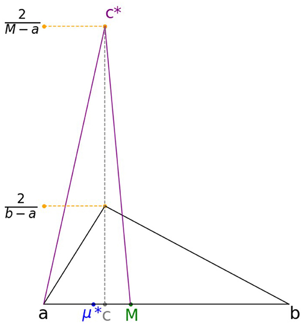
Figure 6. Geometric interpretation for H(M).

In Table 2, we present additional results for comparing standard and mean absolute deviations for normalized triangular distributions for c = {0, 0.25, 0.5, 0.75, 1}. These comparisons are further illustrated in Figure 7.

TABLE 2

Table 2. A comparison of standard and mean absolute deviations.

FIGURE 7

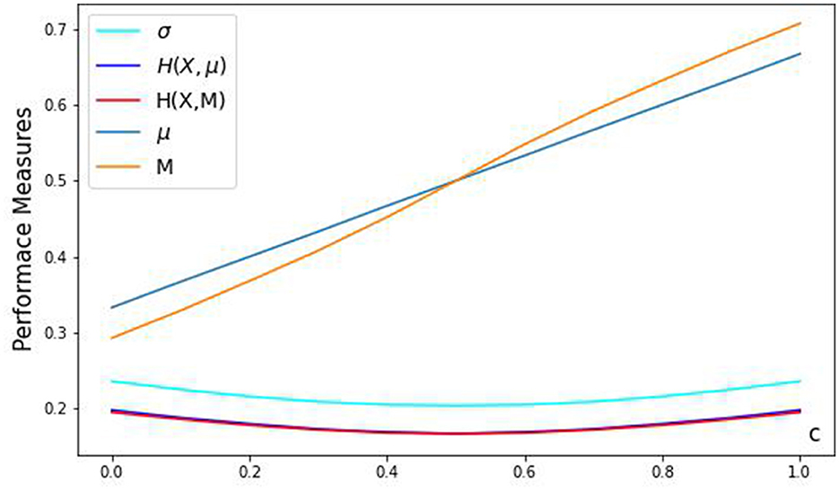
Figure 7. Comparison of performance measures.

As a specific example, consider the symmetric triangular distribution with a = 0, b = 1 and c = 1/2. For this distribution, μ = M = 1/2. The standard deviation $\sigma =\sqrt{2}/6$. The mean absolute deviations H(μ) = H(M) = 1/6. The case c = 1/2 corresponds to the distribution X = (U₁ + U₂)/2 of the mean of the sum of two independent standard uniform variables U₁ and U₂. For these uniform variables, the mean is μ(U₁) = μ(U₂) = 1/2, standard deviation $\sigma (U_1)=\sigma (U_2)=1/(2\sqrt{3})$ and MAD deviation H(U₁, 1/2) = H(U₂, 1/2) = 1/4. We note that ${\sigma }^2(X)={\sigma }^2(U_1/2)+{\sigma }^2(U_2/2)$ but H(1/2) ≠ H(U₂/2, 1/2) + H(U₂/2). From this, we see that, unlike variances, the mean absolute deviation is not additive for the sum of independent random variables. We also note that for the triangular distribution, its standard deviation $\sigma (\text{triangle})=\sqrt{2}/6$ is much larger than the standard deviation of a (normalized) uniform $\sigma (\text{uniform})=\sqrt{3}/6$.

4 Estimation of parameters with mean absolute deviation

In this section, we address the issue of estimating the parameters of this distribution. We could consider several methods to estimate parameters a, b, and c such as maximum likelihood estimation [5, 11], quantiles [4, 12], method of moments or other widely used methods in statistics.

However, we must remember that we assume limited sample data for these distributions. Therefore, the computations based on quantiles may not be very accurate or practical. There are difficulties in using maximum likelihood estimation for triangular distributions as well [13, 14]. One difficulty is that the original density function f(x) in Equation (1) has a “sharp” corner at point c where it does not have a derivative.

4.1 Mean-based and midrange-based estimation of parameters

The simple relationship μ = (a + b + c)/3 in Equation (2) for the mean μ suggests the following simple procedure to estimate the parameters. If we have a set of n data points x₁, …, x_n then we have the following:

1. compute $a^{*}=min\left\{x_i\right\}$ and $b^{*}=max\left\{x_i\right\}$

2. compute the sample mean ${\mu }^{*}=(x_1+\cdots +x_n)/n$

3. compute the mode c^* = 3μ^*−(a^* + b^*)

An even simpler procedure would be to use the mid-range estimator for μ (i.e., assume a symmetric triangle distribution), and proceed as follows:

1. compute $a^{*}=min\left\{x_i\right\}$ and $b^{*}=max\left\{x_i\right\}$

2. estimate the sample mean by mid-range μ^* = (a^* + b^*)/2

3. compute the mode c^* = 3μ^*−(a^* + b^*)

However, the mean μ^* is sensitive to outlier values. However, the mean is more sensitive to outlier values than the median. We, therefore, suggest an alternative method based on the sample median M^* and H(M^*).

4.2 MAD (around median)-based estimation of parameters

Recall that for the median M, we have shown c ≤ (a + b)/2 ⇔ M ≤ c. Combining this with expressions for H(M) in Equation (13), we obtain

$\begin{array}{ll}H(M)=\{\begin{array}{ll}(2M-a-c)/3\hfill & M\le (a+b)/2\hfill \\ (b+c-2M)/3\hfill & M\ge (a+b)/2\hfill \end{array}& (15)\end{array}$

The above results suggest the following estimation procedure:

1. compute $a^{*}=max\left\{x_i\right\}$ and $b^{*}=max\left\{x_i\right\}$

2. compute the sample median M^*

3. compute the mean absolute deviation H(M^*) from the (estimated sample) median M^*

$\begin{array}{ll}H(M^{*})=\frac{1}{n}{\displaystyle \sum _{i=1}^n}|x_i-M^{*}|& (16)\end{array}$

4. from Equation (15) compute the mode c^* as follows

$\begin{array}{ll}{c}^{*}=\{\begin{array}{ll}2M^{*}-3H(M^{*})-a^{*}\hfill & M^{*}\le (a^{*}+b^{*})/2\hfill \\ 2M^{*}+3H(M^{*})-b^{*}\hfill & M^{*}\ge (a^{*}+b^{*})/2\hfill \end{array}\hfill & (17)\end{array}$

This procedure is more stable and less sensitive to outliers than the simple procedure based on the means. This is illustrated by a numerical example below.

4.3 A numerical example for parameter estimation

We present a numerical example of civil engineering data of 85 hauling times presented in [11]. The data is as follows:

$\begin{array}{l}\text{X = {4.79, 4.75, 5.40, 4.70, 6.50, 5.30, 6.00, 5.90, 4.80, 6.70, 6.00, 4.95, 7.90, }\\ \text{ 5.40, 3.50, 4.54, 6.90, 5.80, 5.40, 5.70, 8.00, 5.40, 5.60, 7.50, 7.00, 4.60,}\\ \text{ 3.20, 3.90, 5.90, 3.40, 5.20, 5.90, 4.40, 5.20, 7.40, 5.70, 6.00, 3.60, 6.20,}\\ \text{ 5.70, 5.80, 5.90,6.00, 5.15, 6.00, 4.82, 5.90, 6.00, 7.30, 7.10, 4.73, 5.90,}\\ \text{ 3.60, 6.30, 7.00, 5.10,6.00, 6.60, 4.40, 6.80, 5.60, 5.90, 5.90, 8.60,}\\ \text{ 6.00, 5.80,5.40, 6.50, 4.80, 6.40, 4.15, 4.90, 6.50, 8.20, 7.00, 8.50,}\\ \text{ 5.90, 4.40, 5.80, 4.30, 5.10, 5.90, 4.70, 3.50, 6.80}\}\end{array}$

The mean of this data is μ^* = 5.69, and the standard deviation is σ^* = 1.16. The Gaussian estimation is then c^* = 5.69.

The maximum likelihood estimation of parameters presented in Dorp and Kotz [5] gives the following results:

$\begin{array}{ll}{a}^{*}=2.87,b^{*}=8.80,c^{*}=5.80& (18)\end{array}$

Let us estimate the parameters using the mean-based and MAD-based algorithm.

We start with the mean-based algorithm.

1. compute $a^{*}=min\left\{x_i\right\}=3.2$ and $b^{*}=max\left\{x_i\right\}=8.60$

2. compute the sample mean μ^* = 5.69

3. compute the mode c^* = 3μ^* − (a^* + b^*) = 5.27

Therefore, the mean-based algorithm gives the following:

$\begin{array}{ll}{a}^{*}=3.2,b^{*}=8.6,c^{*}=5.27& (19)\end{array}$

If we consider using the mid-range estimation, then we proceed as follows:

1. compute $a^{*}=min\left\{x_i\right\}=3.2$ and $b^{*}=max\left\{x_i\right\}=8.60$

2. estimate the mean by mid-range μ^* = (a + b)/2 = 5.9

3. compute the mode c^* = 3μ^*−(a^* + b^*) = 5.9

Therefore, the mid-range estimation gives the following:

$\begin{array}{ll}{a}^{*}=3.2,b^{*}=8.6,c^{*}=5.9& (20)\end{array}$

Next, we consider the MAD-based approach

1. compute $a^{*}=max\left\{x_i\right\}=3.2$ and $b^{*}=max\left\{x_i\right\}=8.60$

2. compute the sample median M^* = 5.80

3. compute the mean absolute deviation H(M^*) = 0.88 (from the median)

4. the midpoint (a^* + b^*)/2 = 5.9 is greater than M^*. Therefore, from Equation (17) we compute the mode c^* = (2M^* − 3H(M^*)) − a^* = 5.75

Therefore, the MAD-based algorithm gives the following:

$\begin{array}{ll}{a}^{*}=3.2,b^{*}=8.6,c^{*}=5.75& (21)\end{array}$

We summarize our results from Equations (18–21) in Table 3 where we also added the estimated standard deviation σ^* [computed from Equation (2)]

TABLE 3

Table 3. Comparison of estimation for the numerical example.

Examining Table 3, we see that both mean-based, symmetric PDF and MAD-based procedures give the same estimates for a^* and b^*. These are within about 10% relative errors when compared to the values computed by maximum likelihood in Equation (18). However, the estimate for mode c^* using mean-absolute deviation is much closer to the estimate obtained by maximum likelihood estimation (5.75 vs. 5.80 or about 1% relative error) than the other methods. The estimated standard deviation by MAD-based method is much lower than the the one obtained by the maximum likelihood estimation (1.10 vs. 1.21). At the same time, the MAD-based procedure is computationally much simpler than fitting parameters using the maximum likelihood estimation.

We may consider other methods, based on quantiles. One such method presented in [12] assumes that the most likely value is given and solves for parameters a^* and b^* by numerically solving two quadratic equations corresponding to 5 and 95% quantiles. We could consider another approach: if we have the empirical quartiles $Q_1^{*}$, $Q_3^{*}$, we can compute the interquartile range $I=(Q_3^{*}-Q_1^{*})$. One can then use the Friedman-Diaconis rule [15] to compute the bin width as 2I/n^3/2, construct the empirical histogram and estimate c^* by the midpoint of the most frequent bin. From this, we can solve for a^* and b^* using $Q_1^{*}$, $Q_3^{*}$, and c^*.

However, these methods are pretty complex and require good estimates of the quantiles. In practice, the triangle distributions are often used when there is limited sample data available. For these reasons, the triangle distribution has been called a “lack of knowledge” distribution. Therefore, with small sample sizes, it is not feasible to consider many such methods. By contrast, the suggested MAD-based method for parameter estimation is much simpler computationally.

Let us now illustrate outlier detection using the above example. The simple classical approach is to use mean μ^* and standard deviation σ^* and look for outliers as values below the low bound L = (μ^*− 2σ^*) and above the upper bound U = (μ^* + 2σ^*). The MAD approach would be to use the estimated median M^* and MAD (around median) H^* and look for outlier values outside the low bound L = (M^* − 2H^*) and above the upper bound U = (M^* + 2H^*). We can also consider the simple non-parametric method of Tukey using quartiles [16]. In Tukey's method we compute the quartiles Q₁ and Q₃, compute the interquartile range I = (Q₃ − Q₁) and look for outlier values outside the low bound L = Q₁− 1.5I and above the upper bound U = Q₃ + 1.5I. We present a comparison of outlier detection for the above numerical example in Table 4.

TABLE 4

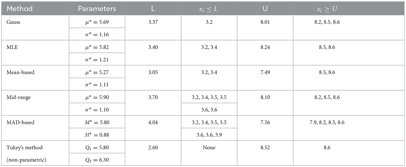
Table 4. Comparison of outlier detection methods.

We note that the lower and upper bounds for the above outlier detection methods can be constructed using a compass and straightedge. One may consider other methods for outlier detection such as Grubbs tests of Gauss pdfs [17] for one-sided and two-sided detection of outliers. This work is only the first step to using the described estimators of triangle distributions. In the future, we aim to address other issues such as the description of errors and uncertainties in measurements, estimation with small numbers of samples, and other rules for detecting and rejecting the outliers.

We conclude this section with a small Monte Carlo simulation study. We considered n = 10, 20, 30, 40, 50. For each n, we ran 100 simulations where we chose c at random in (0, 1) and generated n numbers according to standard triangular distribution (using the Scientific Python library). We then estimated c by maximum likelihood and by the suggested method using H(μ) and H(M). We computed the mean of the relative error for each n and summarized the results in the Table 5. As we can see, for large n the accuracy of the median-based method is always better than using the maximum Likelihood estimation. The proposed method is much simpler computationally.

TABLE 5

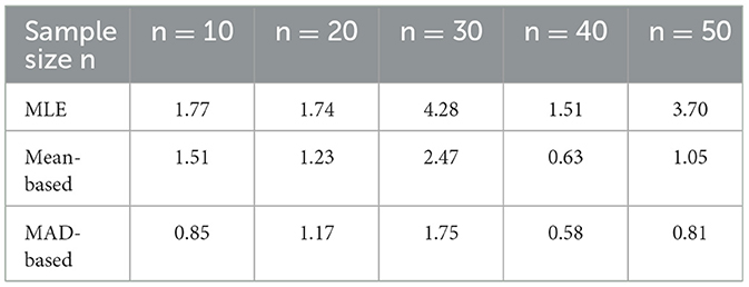
Table 5. Relative errors in estimating mode c by Monte Carlo.

5 Estimation of tail probabilities with deviations

We now turn to compute some tail probabilities. The quadratic form of the CDF F(x) for the triangular distribution (Equation 1) results in a simple quadratic form of tail probabilities. For example, for any ϵ < min{c − a, b − c} we have

$\begin{array}{l}P(|X-c|\ge ϵ)=P(X\le c-ϵ)+P(X\ge c+ϵ)=F(c-ϵ)\\ +(1-F(c+ϵ))=\frac{{((c-a)-ϵ)}^2}{(b-a)(c-a)}+\frac{{((b-c)-ϵ)}^2}{(b-a)(b-c)}& (22)\end{array}$

The above probability can be constructed geometrically. Recall that one of our assumptions is having a segment of unit length. This allows us to compute both the products and ratios of segments.

Let us examine how the MAD deviations can be used to estimate tail probabilities. The most general bound for any distribution (with finite variance) is the Chebyshev's inequality [18]:

$\begin{array}{ll}P(|X-\mu |\ge k\sigma )\le \frac{1}{k^2}& (23)\end{array}$

This inequality is useful for k ≥ 1. This inequality follows from the so-called Pearson inequality [19] with r = 2

$\begin{array}{ll}P(|X-\mu |\ge k{V}_r^{1/r})\le \frac{1}{k^2},\text{ where }{V}_r=\text{E}(|X-\mu {|}^r)& (24)\end{array}$

For r = 1, a much less-known inequality exists for bounds in terms of mean absolute deviation H(μ) from the mean, namely

$\begin{array}{ll}P(|X-\mu |\ge kH(\mu ))\le \frac{1}{k}& (25)\end{array}$

Similarly, there is an inequality in terms of the mean absolute deviation from the median H(M) given by [9]

$\begin{array}{ll}P(|X-M|\ge kH(M))\le \frac{1}{k}& (26)\end{array}$

Let us compute bounds based on the MAD deviation. First, define δ = H(μ)/σ. Note that for all distributions we have H(μ) ≤ σ and therefore δ ≤ 1. We can re-write the MAD-based inequality for H(μ) in Equation (25) in terms of σ as follows

$\begin{array}{ll}P(|X-\mu |\ge k\sigma )=P(|X-\mu |\ge \frac{k\sigma }{H(\mu )}·H(\mu ))\le \frac{\delta }{k}& (27)\end{array}$

Also, we can consider the Peek inequality [20]

$\begin{array}{ll}P(|X-\mu |\ge k\sigma )\le \frac{1-{\delta }^2}{k^2-2k\delta +1}& (28)\end{array}$

Comparing Equations (23) and (27) we find that MAD-based upper bound for H(μ) is lower than Chebyshev's upper bound for 1 ≤ k ≤ 1/δ. Comparing Equations (27) and (28) we find that Peek inequality is lower than both MAD and Chebyshev for k > 1/δ.

We can now apply these bounds to triangular distribution. Since σ, H(M), and H(μ) are shift-invariant and multiplicative, we can consider only the standard triangular distribution with a = 0 and b = 1. Consider again the symmetric case c = 1/2. From Table 2, we have μ = 1/2, $\sigma =\sqrt{6}/12$, H(μ) = 1/6, and $\delta =\sqrt{6}/3$. The tail probability from Equation (1) is

$\begin{array}{ll}P(|X-\mu |\ge k\sigma )=1+\frac{k^2}{6}-\frac{k\sqrt{6}}{3}& (29)\end{array}$

Let us now consider bounds using deviations. Therefore, from Equation (27), the MAD-based bound for the tail probability in standard symmetric triangular distribution is

$\begin{array}{ll}P(|X-\mu |\ge k\sigma )\le \frac{\sqrt{6}}{3k}& (30)\end{array}$

Comparing this with Chebyshev's inequality (23) we find that the MAD-based bound is sharper for $k\le 1/\delta =\sqrt{6}/2\approx 1.22$. The Peek inequality in Equation (28) (with $\delta =\sqrt{6}/3$) gives the following:

$\begin{array}{ll}P(|X-\mu |\ge k\sigma )\le =\frac{1}{3k^2-2k\sqrt{6}+3}& (31)\end{array}$

This gives us a sharper bound than MAD for the same value $k=\sqrt{6}/2$.

In Figure 8 we compare the exact value of tail probabilities (Equation 29), the Chebyshev bound (Equation 23), the MAD bound (Equation 27), and the Peek bound (Equation 28). For $k<\sqrt{6}/2$ the MAD bound in Equation (27) gives a lower bound than either Chebyshev or Peek inequalitiy. For $k>\sqrt{6}/2$, both Chebyshev and Peek give lower values with the Peek inequality being the sharper bound. We note that none of these bounds give good approximations, especially for larger k. For example, at point $k=\sqrt{6}/2$ the Chebyshev, MAD, and Peek bounds are 2/3 whereas the exact value from Equation (29) is 0.25. We will consider other Chebyshev's type inequalities [21] and the inequalities based on the median in future work.

FIGURE 8

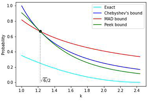
Figure 8. Comparison of tail probabilities for the standard symmetric case.

6 Geometry of quartile deviations

In quantile statistics, one often uses half of the interquartile range (IQR) as a measure of deviation [1]. If the first and third quartiles are given by $Q_1=F^{-1}(1/4)$ and $Q_3=F^{-1}(3/4)$ respectively then the interquartile range I = (Q₃ − Q₁). The quartile deviation G is then G = (Q₃ − Q₁)/2. This has a very simple interpretation. Since G = ((Q₃ − M) + (M − Q₁))/2, we can interpret G as the average distance from the median to the other two quartiles.

To compute the quartiles and to derive the expression for G for triangular distribution, it will be enough to consider the case a ≤ c ≤ (b − a)/2. If X ~ Tr(a, b, c) consider the random variable Y = (a + b) − X. This random variable has a triangular distribution Y ~ Tr(a, b, (b + a) − c). Its quartiles and median are related to the quartiles and median of X by simple relationships

$\begin{array}{c}{Q}_1(X)-a=b-Q_3(Y),M(X)-a=b-M(Y),Q_3(X)-a\\ =b-Q_1(Y)& (32)\end{array}$

For a geometric interpretation of the quartiles, we will find it convenient to find their distances from a or b. We compute the general expression for these distances by considering the following cases:

• Case 1 (c = a): For this case, the cumulative distribution function F(x) = 1 − (b − x)²/(b − a)². The first quartile Q₁, the median M and the third quartile are found from solving F(x) = q for q = 1/4, q = 1/2 and q = 3/4 respectively. Since x > c we use the second equation in Equation (3) and obtain:

$\begin{array}{r}(b-Q_1)=\frac{\sqrt{3}}{2}(b-a),(b-M)=\frac{\sqrt{2}}{2}(b-a),(b-Q_3)\\ =\frac{(b-a)}{2}\end{array}$

This suggests the following geometric construction for quartiles:

1. construct 60°/30° right triangle T with hypotenuse (b − a)

2. compute the other two sides of T: $l_1=(b-a)\sqrt{3}/2$ and l₂ = (b − a)/2

3. l₁ = (Q₁ − b) and l₂ = (b − Q₃) are distances of quartiles from b

4. the difference (l₁ − l₂) is the interquartile range I = (Q₃ − Q₁)

• Case 2 (0 < c ≤ (a + b)/2): from Equation (2.2) in Section 2 we have M ≥ c. And since Q₃ > M we obtain the following for the median M and the third quartile Q₃:

$\begin{array}{l}(b-M)=\frac{\sqrt{2}}{2}\sqrt{(b-a)(b-c)},(b-Q_3)=\frac{1}{2}\sqrt{(b-a)(b-c)}\end{array}$

What about the first quartile Q₁? If Q₁ ≤ c then from Equation (3) we have

$\begin{array}{l}a+\frac{1}{2}\sqrt{(b-a)(c-a)}\le c\Rightarrow c\ge a+\frac{(b-a)}{4}\end{array}$

Similarly, for c < a + (b − a)/4 we have Q₁ > c. Therefore, from Equation (3) we obtain for Q₁:

$\begin{array}{l}\{\begin{array}{ll}(b-Q_1)=\frac{\sqrt{3}}{2}\sqrt{(b-a)(b-c)}\hfill & a<c<a+\frac{(b-a)}{4}\hfill \\ (Q_1-a)=\frac{1}{2}\sqrt{(b-a)(c-a)}\hfill & a+\frac{(b-a)}{4}\le c<\frac{(a+b)}{2}\hfill \end{array}\hfill \end{array}$

This suggests the following geometrical construction for quartiles.

For the case a < c < a + (b − a)/4 we do the following:

1. compute the geometric mean $l_1=\sqrt{(b-a)(b-c)}$

2. construct a 60°/30° right triangle T with hypotenuse l₁

3. compute the other two sides of this triangle: $l_2=l_1\sqrt{3}/2$ and l₃ = l₁/2

4. l₂ = (b − Q₁) and l₃ = (b − Q₃) are distances from quartiles from b

5. the difference of sides (l₁ − l₂) is the interquartile range I = (Q₃ − Q₁)

For the case a + (b − a)/4 ≤ c < (a + b)/2 the construction is similar except that we use an additional 45°/45° triangle as follows:

1. compute the geometric mean $\sqrt{(b-a)(c-a)}$

2. bisect this geometric mean to obtain l₁

3. compute the geometric mean $\sqrt{(b-a)(b-c)}$

4. bisect this geometric mean to obtain l₂

5. l₁ = (Q₁ − a) and l₂ = (b − Q₃) are distances from quartiles from a and b respectively

6. the difference (b − a) − (l₁ + l₂) is the interquartile range I = (Q₃ − Q₁)

• Case 3 ((a + b)/2 ≤ c < b): In this case, from Equation (32) we obtain

$\begin{array}{l}(Q_1-a)=\frac{1}{2}\sqrt{(b-a)(c-a)},(M-a)=\frac{\sqrt{2}}{2}\sqrt{(b-a)(c-a)}\end{array}$

And for Q₃, we can show (similar to the previous case)

$\{\begin{array}{ll}(b-Q_3)=\frac{1}{2}\sqrt{(b-a)(b-c)}\hfill & \frac{(a+b)}{2}<c<a+\frac{3(b-a)}{4}\hfill \\ (Q_3-a)=\frac{\sqrt{3}}{2}\sqrt{(b-a)(c-a)}\hfill & a+\frac{3(b-a)}{4}\le c<b\hfill \end{array}$

The geometric construction for this case is similar to Case 2.

• Case 4 (c = b): From Case c = a and Equation (32) we obtain

$\begin{array}{l}(Q_1-a)=\frac{1}{2}(b-a),(M-a)=\frac{\sqrt{2}}{2}(b-a),(Q_3-a)=\frac{\sqrt{3}}{2}(b-a)\end{array}$

The geometric construction for this case is similar to Case 1.

Combining the expressions for the quartiles from the above cases, we can write a general expression for the quartile deviation:

$\begin{array}{ll}G=\{\begin{array}{ll}\frac{(\sqrt{3}-1)(b-a)}{4}\hfill & c=a\text{ or }c=b\hfill \\ \frac{(\sqrt{3}-1)\sqrt{(b-a)(c-a)}}{4}\hfill & a<c<a+\frac{(b-a)}{4}\hfill \\ \hfill & \text{ or }a\hfill \\ \hfill & +\frac{3(b-a)}{4}\le c<b\hfill \\ \frac{(b-a)}{2}-\frac{\sqrt{b-a}}{4}\left(\sqrt{b-c}+\sqrt{c-a}\right)\hfill & a+\frac{(b-a)}{4}\hfill \\ \hfill & \le c<a+\frac{3(b-a)}{4}\hfill \end{array}& (33)\end{array}$

From the above, we have the following geometrical interpretation: the distances of the quartiles Q₁ and Q₃ can be computed as sides of right triangles. The difference in these distances is the interquartile range I. The quartile deviation G is one-half of this difference. The geometric interpretation of G can be demonstrated in Figure 9.

FIGURE 9

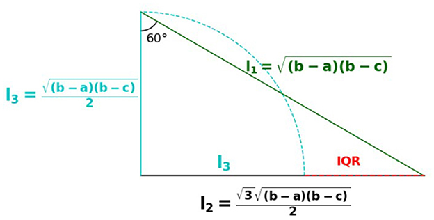
Figure 9. Geometric interpretation for quartile deviation.

For the standard triangular distribution with a = 0 and b = 1, we can re-write the above as

$\begin{array}{ll}G=\{\begin{array}{ll}(\sqrt{3}-1)/4\hfill & c=0\text{\hspace{1em}or\hspace{1em}}c=1\hfill \\ (\sqrt{3}-1)\sqrt{c}/4\hfill & 0<c<1/4\text{\hspace{1em}or\hspace{1em}}3/4\le c<1\hfill \\ 1/2-\left(\sqrt{1-c}+\sqrt{c}\right)/4\hfill & 1/4\le c<3/4\hfill \end{array}& (34)\end{array}$

In Table 6 we compute the quartiles and the quartile deviation for the normalized triangular distribution with a = 0 and b = 1 for c = 0, c = 1/4, c = 1/2, c = 3/4 and c = 1.

TABLE 6

Table 6. Quartiles, quartile deviations and comparison of deviation measures for normalized triangular distributions.

7 Comparison of deviation measures

In this section, we present some results in comparison of the four deviation measures

1. standard deviation σ

2. mean absolute deviation (about mean) H(μ)

3. mean absolute deviation (about median) H(M)

4. quartile deviation G

All these measures are shift-invariant. it is easy to show that scaling the data by any constant k, changes these deviation measures by |k|. Therefore, without loss of generality, it would be sufficient to compare these measures for the standard triangular distribution with a = 0 and b = 1.

In Table 7, we present a comparison for different values of c.

TABLE 7

Table 7. A comparison of deviation measures.

From our discussion in Section 7 we know that H(M) ≤ H(μ) ≤ σ. We will first prove that G < H(M). By symmetry, we will only need to prove G < H(M) for 0 ≤ c ≤ 1/2. We need to consider the following cases:

• Case 1: c = 0 or c = 1: From Equations (14) and (34) we have

$\begin{array}{l}H(M)-G=\frac{(2-\sqrt{2})}{3}-\frac{(\sqrt{3}-1)}{4}>0\end{array}$

• Case 2: 0 < c ≤ 1/4: For this case, (2 − c) ≥ 7/4, $\sqrt{c}\le 1/2$, and $\sqrt{2(1-c)}\le \sqrt{2}$. Therefore, from Equations (14) and (34) we have

$\begin{array}{l}\begin{array}{cc}H(M)-G& >\frac{(7/4-\sqrt{2})}{3}-\frac{(\sqrt{3}-1)}{8}>0\end{array}\end{array}$

• Case 3: 1/4 ≤ c ≤ 1/2: In this case, (2 − c) ≥ 3/2, $\sqrt{c}\ge 1/2$, $\sqrt{1-c}\ge \sqrt{3}/2$, and $\sqrt{2(1-c)}\le \sqrt{2}/2$. Therefore, from Equations (14) and (34) we have

$\begin{array}{r}\begin{array}{r}H(M)-G\ge \frac{(3/2-\sqrt{2}/2)}{3}-\frac{1}{2}\\ +\frac{(\sqrt{3}/2+1/2)}{4}=\frac{(1+\sqrt{3})}{8}-\frac{\sqrt{2}}{6}>0\end{array}\end{array}$

Therefore, we have the following relationship between these deviation measures:

$\begin{array}{ll}G<H(M)\le H(\mu )\le \sigma & (35)\end{array}$

In Figure 10, we show the comparison between these four deviation measures for the standard triangular distribution. We note that across this range, both H(μ) and H(M) are practically identical. At midpoint c = 1/2 they achieve their minimum value and are equal: H(M) = H(μ) = 1/6, whereas at c = 0 or c = 1, they are within 2% of each other by relative value: H(μ) = (2/3)⁴ ≈ 0.198 vs. $H(M)=(2-\sqrt{2})/3\approx 0.195$. The standard deviation varies from $\sigma =\sqrt{2}/6\approx 0.236$ for c = 0 or c = 1. It achieves its minimum value $\sigma =\sqrt{6}/12\approx 0.204$ at midpoint c = 1/2. Therefore, compared to mean absolute deviations H(μ) and H(M), the standard deviation is σ is about 20% higher than the mean absolute deviation H(M). If we consider the quantile deviation G, it has the maximum value $G=(\sqrt{3}-1)/4\approx 0.183$ for c = 0 and c = 1. For these values of c, H(M) ≈ 0.195, and therefore, the quartile deviation is about 6% lower than H(M) It decreases as c increases from c = 0 to c = 1/2 and achieves its minimum value at the midpoint: $G=(2-\sqrt{2})/4\approx 0.146$. Compared with the mean absolute deviation H(M) ≈ 0.167 at the midpoint, the quartile deviation is about 13% lower. We can conclude that, on average, the quartile deviation is about 10% lower than the mean absolute deviation (about median) H(M). In contrast, the standard deviation is about 20% higher than H(M). At the same time, the quartile deviation has higher volatility. We can compare these measures' volatilities V(·) by examining their range relative to their minimum value (at point c = 1/2). In percentage terms for the four deviation measures, we obtain:

$\begin{array}{l}V(\sigma )=15.5\%,V(H(\mu ))=18.5\%,V(H)=17.2\%,V(G)=25.0\%\end{array}$

FIGURE 10

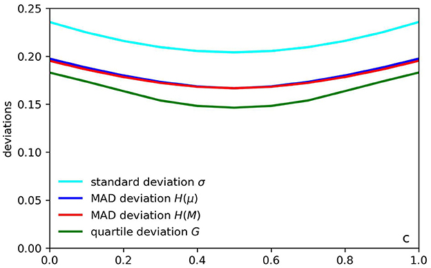
Figure 10. A comparison of deviations for standard triangular distribution (a = 0, b = 1).

The volatilities of standard and mean absolute deviations are close to each other by value and are around 15–18%. In contrast, the volatility of the quartile deviation is much higher at about 25%.

We should emphasize that, in practice, we have a limited number of points. As a result, it may be difficult to get accurate estimates for the quartiles to compute the quartile deviation. Therefore, from a practical standpoint, it is better to compute the mean absolute deviation and use it to compute the parameters of the distributions, as we have suggested.

8 Conclusion

In this paper, we presented a detailed comparison of deviation metrics for the the triangular distribution. We derived a novel formula for the mean absolute deviation from the median H(M) and suggested a new estimation procedure of parameters. Most performance measures have simple geometric interpretation and can be constructed by compass and straightedge. Future work will consider applying these ideas to extensions of triangular distributions such as PERT and two-sided power distributions widely used in risk analysis.

Data availability statement

The original contributions presented in the study are included in the article/supplementary material, further inquiries can be directed to the corresponding author.

Author contributions

EP: Writing—original draft, Writing—review & editing. YW: Writing—original draft, Writing—review & editing.

Funding

The author(s) declare that no financial support was received for the research, authorship, and/or publication of this article.

Acknowledgments

The authors thank metropolitan College of Boston University for their support.

Conflict of interest

The authors declare that the research was conducted in the absence of any commercial or financial relationships that could be construed as a potential conflict of interest.

Publisher's note

All claims expressed in this article are solely those of the authors and do not necessarily represent those of their affiliated organizations, or those of the publisher, the editors and the reviewers. Any product that may be evaluated in this article, or claim that may be made by its manufacturer, is not guaranteed or endorsed by the publisher.

References

1. Johnson NL, Kotz S. Distributions in Statistics. New York: J Wiley. (1970).

Google Scholar

2. Fairchild KW, Misra L, Shi Y. Using triangular distribution for business and finance simulations in excel. J Financ Applic. (2016) 42:313–36.

Google Scholar

3. Hopkinson M. Three point estimates: a brief guide, practical risk management series. PM World J. (2022) 6:1–3.

Google Scholar

4. Johnson D. Triangular approximations for continuous random variables in risk analysis. J Oper Res Soc. (2002) 53:457–67. doi: 10.1057/palgrave.jors.2601330

CrossRef Full Text | Google Scholar

5. Dorp JR, Kotz S. A novel extension of the triangular distribution and its parameter estimation. Statistician. (2002) 51:63–79. doi: 10.1111/1467-9884.00299

CrossRef Full Text | Google Scholar

6. Johnson D. The triangular distribution as a proxy for the beta distribution in risk analysis. Statistician. (1997) 46:387–98. doi: 10.1111/1467-9884.00091

CrossRef Full Text | Google Scholar

7. Johnson NL, Kotz S. Non-smooth sailing or triangular distributions revisited after some 50 years. Statistician. (1999) 48:179–87. doi: 10.1111/1467-9884.00180

CrossRef Full Text | Google Scholar

8. Gorard S. Revisiting a 90-year-old debate: the advantages of the mean deviation. Br J Educ Stud. (2005) 53:417–30. doi: 10.1111/j.1467-8527.2005.00304.x

CrossRef Full Text | Google Scholar

9. Pham-Gia T, Hung TL. The mean and median absolute deviations. J Mathem Comput Model. (2001) 34:921–36. doi: 10.1016/S0895-7177(01)00109-1

CrossRef Full Text | Google Scholar

10. Pinsky E, Klawansky S. MAD (about Median) vs. quantile-based alternatives for classical standard deviation, skew, and kurtosis. Front Appl Mathem Statist. (2023) 9:1206537. doi: 10.3389/fams.2023.1206537

CrossRef Full Text | Google Scholar

11. AbouRizk SM. Input Modeling for Construction Simulation. PhD Thesis, Purdue University Ann Arbor, MI: UMI Dissertation Services. (1990).

Google Scholar

12. Keefer DL, Bodily SE. Three-point approximations for continuous random variables. Manage Sci. (1983) 29:595–609. doi: 10.1287/mnsc.29.5.595

CrossRef Full Text | Google Scholar

13. Kotz S, Dorp JR. Beyond Beta: Other Continuous Families of Distributions with Bounded Support and Applications. New Jersey: World Scientific Publishing. (2004). doi: 10.1142/5720

CrossRef Full Text | Google Scholar

14. Oliver EH. A maximum likelihood oddity. Am Stat. (1972) 26:43–4. doi: 10.1080/00031305.1972.10478930

CrossRef Full Text | Google Scholar

15. Friedman D, Diaconis P. On the histogram as a density estimator L₂ theory. Probab Theory Relat Fields. (1981) 57:453–76. doi: 10.1007/BF01025868

CrossRef Full Text | Google Scholar

16. Tukey J. Exploratory Data Analysis. London, UK: Pearson Publishing. (1977).

Google Scholar

17. Grubbs FE. Procedures for detecting outlying observations in samples. Technometrics. (1969) 11:1–21. doi: 10.1080/00401706.1969.10490657

CrossRef Full Text | Google Scholar

18. Feller JJ. Probability Theory and Applications. New York: J Wiley. (1956).

Google Scholar

19. Stuart A, Ord JK. Kendalls Advanced Theory of Statistics. vol 1 New York: Oxford University Press. (1987).

Google Scholar

20. Peek RL. Some new theorems on limits of variation. Bull Am Mathem Soc. (1933) 39:953–9. doi: 10.1090/S0002-9904-1933-05780-4

CrossRef Full Text | Google Scholar

21. Savage IR. Probability inequalities of the tchebycheff type. J Res Nat Bureau Stand B Mathem Phys. (1961) 65B:211–226. doi: 10.6028/jres.065B.020

CrossRef Full Text | Google Scholar

22. Bloomfield P, Steiger WL. Least Absolute Deviations: Theory, Applications and Algorithms. Boston: Birkhauser. (1983). doi: 10.1007/978-1-4684-8574-5

CrossRef Full Text | Google Scholar

23. Shad SM. On the minimum property of the first absolute moment. Am Stat. (1969) 23:27. doi: 10.2307/2682577

CrossRef Full Text | Google Scholar

24. Schwertman NC, Gilks AJ, Cameron J. A Simple noncalculus proof that the median minimizes the sum of the absolute deviations. Am Stat. (1990) 44:38–41. doi: 10.2307/2684955

CrossRef Full Text | Google Scholar

Appendix

Appendix A: Details on computation of mean absolute deviations

We start by establishing a lower and upper bound for mean absolute deviations. Since f(x) ≥ 0, is integrable and E(X) < ∞ we have −|x − p|f(x) ≤ (x − p)f(x) ≤ |x − p|f(x) and, therefore, we obtain

$\begin{array}{ll}H(p)={\displaystyle {\int }_X}|x-p|f(x)dx\ge |{\displaystyle {\int }_X}(x-p)f(x)dx|=|p-\mu |& (36)\end{array}$

To establish an upper bound, we use the well-known fact that H(M) ≤ H(p) for any value of p [22–24]. In particular, if p = μ then H(M) ≤ H(μ).

If we apply Jensen's inequality E(g(X)) ≥ g(μ) to the convex function g(t) = t² (corresponding to σ²) we obtain an upper bound for H(M):

$\begin{array}{ll}{\sigma }^2=\text{E}(g(|X-\mu |))\ge g(\text{E}(|X-\mu |))=[\text{E}(|X-\mu |){]}^2\ge H^2(M)& (37)\end{array}$

It follows from Equation (37) that σ ≥ H(μ) ≥ H(M).

We now deriving a formula for H(p). We will find it convenient to define and evaluate the following auxiliary integrals I₁(t) and I₂(t). For a ≤ t ≤ c define

$\begin{array}{r}{I}_1(t)={\displaystyle {\int }_t^c}xf(x)dx={\displaystyle {\int }_t^c}\frac{2x(x-a)}{(b-a)(c-a)}dx\\ =\frac{2c^3-2t^3-3a{c}^2+3a{t}^2}{3(b-a)(c-a)}& (38)\end{array}$

and for c ≤ t ≤ b define

$\begin{array}{r}{I}_2(t)={\displaystyle {\int }_c^t}xf(x)dx={\displaystyle {\int }_c^t}\frac{2x(b-x)}{(b-a)(b-c)}dx\\ =\frac{3b{t}^2-3b{c}^2-2t^3+2c^3}{3(b-a)(b-c)}& (39)\end{array}$

To derive a general expression for H(p), we need to consider two cases: p ≥ c and p ≤ c

Case 1: p ≥ c. For this case, we have

$\begin{array}{l}\begin{array}{l}H(p)={\displaystyle {\int }_a^c}(p-x)f(x)dx+{\displaystyle {\int }_c^p}(p-x)f(x)dx+{\displaystyle {\int }_p^b}(x-p)f(x)dx\\ =p\left[{\displaystyle {\int }_a^c}f(x)dx-I_1(a)\right]+\\ p\left[{\displaystyle {\int }_c^p}f(x)dx-I_2(p)\right]+\left[I_2(b)-I_2(p)-p{\displaystyle {\int }_p^b}f(x)dx\right]\\ =I_2(b)-I_1(a)-2I_2(p)+p(2F(p)-1)\end{array}\end{array}$

Case 2: p ≤ c. For this case, we have

$\begin{array}{l}\begin{array}{l}H(p)={\displaystyle {\int }_a^p}(p-x)f(x)dx+{\displaystyle {\int }_p^c}(x-p)f(x)dx+{\displaystyle {\int }_c^b}(x-p)f(x)dx\\ =\left[p{\displaystyle {\int }_a^p}f(x)dx-(I_1(a)-I_1(p))\right]\\ +\left[I_1(p)-p{\displaystyle {\int }_p^c}f(x)dx\right]\\ +\left[I_2(b)-p{\displaystyle {\int }_c^b}f(x)dx\right]\\ =I_2(b)-I_1(a)+2I_1(p)+p(2F(p)-1)\end{array}\end{array}$

From these cases and noting that I₁(a) + I₂(b) = μ, we obtain the following general formula for H(p):

$\begin{array}{ll}H(p)=\{\begin{array}{ll}2I_2(b)-\mu -2I_2(p)+p\left(2F(p)-1\right)\hfill & p\ge c\hfill \\ \mu -2I_1(a)+2I_1(p)+p\left(2F(p)-1\right)\hfill & p\le c\hfill \end{array}\hfill & (40)\end{array}$

We can now compute the median absolute deviations H(μ) and H(M)

1. Computation of H(μ):

There are two cases to consider:

• Case 1: a ≤ c ≤ (a + b)/2 ⇒ μ ≥ c

• Case 2: (a + b)/2 ≤ c ≤ b ⇒ μ ≤ c

From this and Equation (40), we obtain the following general expression for the mean absolute deviation H(μ):

$\begin{array}{ll}H(\mu )=\{\begin{array}{ll}\frac{2{(a+c-2b)}^3}{81(a-b)(b-c)}\hfill & a\le c\le (a+b)/2\hfill \\ \frac{2{(b+c-2a)}^3}{81(a-b)(a-c)}\hfill & (a+b)/2\le c\le b\hfill \end{array}& (41)\end{array}$

2. Computation of H(M): There are two cases to consider:

• Case 1: a ≤ c ≤ (a + b)/2 ⇒ M > c

• Case 2: (a + b)/2 ≤ c ≤ b ⇒ M ≤ c

From this and Equations (4) and (40) we obtain the following general expression for H(M):

$\begin{array}{ll}H(M)=\{\begin{array}{ll}\frac{(b-a)+(b-c)-\sqrt{2(b-a)(b-c)}}{3}\hfill & a\le c\le (a+b)/2\hfill \\ \frac{(b-a)+(c-a)-\sqrt{2(b-a)(c-a)}}{3}\hfill & (a+b)/2\le c\le b\hfill \end{array}& (42)\end{array}$