Solving a fractional diffusion PDE using some standard and nonstandard finite difference methods with conformable and Caputo operators

Introduction: Fractional diffusion equations offer an effective means of describing transport phenomena exhibiting abnormal diffusion pat-terns, often eluding traditional diffusion models.

Methods: We construct four finite difference methods where fractional derivatives are approximated using either conformable or Caputo operators.

Results: Stability of the proposed schemes is analyzed using von Neumann stability analysis, and conditions are established to preserve positivity. Consistency analysis is performed for all methods, and numerical results with fractional parameters (α) set to 0.75, 0.90, 0.95, and 1.0 are presented.

Discussion: The rate of convergence in time for the four methods is computed.

1 Introduction

Fractional partial differential equations (FPDEs) are a generalization of classical partial differential equations (PDEs) by incorporating fractional derivatives of arbitrary order, providing a versatile framework for describing a broad range of phenomena in physical, chemical, biological, and financial processes with anomalous transport mechanisms [1]. These equations capture non-local and non-linear aspects that are not captured by classical PDEs [2]. Real-world physical models often entail substantial uncertainty arising from numerous variables [3].

Solving FPDEs numerically poses challenges due to their inherently non-local and non-linear nature [2, 4, 5].

A fractional diffusion equation can be expressed in the form [1]

$\begin{array}{ll}{}_0{D}_t^{\alpha }u(x,t)=\frac{{\partial }^{2}u(x,t)}{\partial x^2}+f(x,t),& (1)\end{array}$

where t>0, L ≤ x ≤ R, and 0 < α ≤ 1, with initial condition given by Equation 2:

$\begin{array}{ll}u(x,0)=\psi (x),& (2)\end{array}$

and boundary conditions: u(L, t) = f(t), and u(R, t) = g(t), where ${}_0{D}_t^{\alpha }u(x,t)$ in Equation 1 is the Caputo fractional derivative of order α, and is given by Equation 3 as follows:

$\begin{array}{ll}\begin{array}{l}{}_a{D}_t^{\alpha }u(x,t)=\frac{1}{\text{Γ}(m-\alpha )}{\displaystyle {\int }_a^t{(t-\xi )}^{m-\alpha -1}\frac{{\partial }^{m}u(x,\xi )}{\partial {\xi }^m}d\xi ,}\hfill \end{array}& (3)\end{array}$

where m−1 < α < m, m∈ℕ [6].

In the realm of FPDEs, diffusion equation via the Caputo operator can be used in modeling transport of diffusion processes, by offering a profound mechanism for describing memory and hereditary properties of materials and processes. This aspect is crucial for our work with a fractional diffusion experiment, where the traditional integer-order models fall short in capturing the complex dynamics of anomalous diffusion prevalent in many natural and engineering systems. Incorporating the Caputo operator allows for a more accurate representation of the non-local and history-dependent behavior of diffusion processes, enhancing the model's ability to predict and analyze real-world scenarios effectively [7, 8]. Furthermore, the insights from Awadalla et al. [9] and Shaikh and Qureshi [10] shed some light on contributions of the Caputo operator toward modeling complex dynamical systems, including its application in fractional optimal control models and bifurcation analysis of human syncytial respiratory virus transmission dynamics. Awadalla et al. [9] showed the operator's efficacy in applications ranging from fractional optimal control models to the bifurcation analysis of human respiratory virus transmission dynamics, reinforcing the Caputo operator's indispensability in capturing some dynamics of such systems.

Mathematical modeling of pattern formation in coral reefs using fractional differential equations shows an elegant approach to capturing the complex dynamics of ecological systems [11]. Fractional models are particularly adept at describing phenomena with memory effects and spatial heterogeneity, characteristics inherent to ecological patterns observed in coral reefs. A fractional partial differential equation modeling coral reef growth and interaction can be expressed as [12]:

$\begin{array}{l}{\mathcal{D}}_t^{\alpha }N(x,t)=D_N{\nabla }^{2\beta }N(x,t)+R(N,C)-M(N),\end{array}$

where N(x, t) represents the coral population density at location x and time t, D_N is the diffusion coefficient capturing the spread of coral larvae, α and 2β denote the fractional orders of time and space derivatives reflecting memory and spatial dispersal effects, R(N, C) is the growth rate dependent on coral and nutrient concentration C, and M(N) represents natural mortality. Such models allow for understanding of how local interactions and environmental conditions influence large-scale pattern formation, offering insights into conservation strategies and reef resilience [13, 14].

Recent advancements in numerical methods for solving non-linear partial differential equations (PDEs) encompass notable techniques such as the optimal homotopy continuation method [15], variational homotopy method [16], and a hybrid iterative approach [17]. Qureshi et al. [18] used a three-step numerical scheme showing ninth-order convergence in solving non-linear equations. Comparative analyses revealed its superior efficiency when compared to established schemes in computational science. In addition, the authors, in [19], investigated a novel optimal iterative algorithm with fourth-order accuracy tailored for root-finding in real functions.

Analytic solutions of most FPDEs cannot be obtained explicitly. In fact, the closed form solutions for many time-fractional differential equations are not available [1, 20]. Some nonstandard finite difference (NSFD) schemes were first devised by Mickens [21].

The primary merit of the NSFD schemes lies in their ability to overcome the inherent numerical instabilities associated with classical finite difference methods [21]. The development of NSFD methods adheres to some fundamental rules for its practical implementation [22–26]:

(i) The order of discrete derivatives should match the order of the corresponding derivatives in the given differential equation.

(ii) Discrete representations for derivatives typically involve non-trivial denominator functions. For instance:

$\frac{\partial u}{\partial t}\approx \frac{U_{j+1}^n-U_j^n}{\varphi (k,\lambda )},$

where $\varphi (k,\lambda )=k+\mathcal{O}(k^2)$.

Recently, NSFD methods have been constructed by many researchers for solving differential equations. Agarwal and El-Sayed proposed a nonstandard finite difference method and a Chebyshev collocation method to solve a fractional order diffusion equation [27]. Momani et al. [25] constructed a nonstandard implicit Euler method for solving a class of fractional partial differential equations. Tijani and Appadu [28] constructed an unconditionally positive nonstandard finite difference scheme for a mathematical model of biofilm formation on a medical implant. The model employed uses the bistable Allen-Cahn partial differential equation, which is a generalization of Fisher's equation. Appadu and Tijani [29] obtained the numerical solution of a 1-D generalized Burgers-Huxley equation under specified initial and boundary conditions, and they used Forward Time Central Space (FTCS) and a nonstandard finite difference scheme. Agbavon and Appadu [26] constructed a nonstandard finite difference schemes to solve the FitzHugh-Nagumo equation with specified initial and boundary conditions under three different regimes. Kehinde et al. [30] obtained solution to a two-dimensional semilinear singularly perturbed semilinear convection-diffusion problem by constructing a nonstandard finite difference method. Jejeniwa et al. [31] used three methods: the Kowalic-Murty scheme, Lax-Wendroff scheme, and nonstandard finite difference (NSFD) scheme, to solve 1D and 2D convective diffusion equations. They looked at the cases when the advection velocity was much greater than of the diffusion coefficient and when the coefficient of diffusion was much greater than the advection velocity. They also analyzed the dispersion properties of the three methods.

Fractional subdiffusion and superdiffusion are described by the parameter α, which determines the anomalous nature of diffusion. In subdiffusion, α ranges from 0 to 1 (0 < α < 1), indicating that the mean squared displacement (MSD) increases slower than in classical diffusion. This behavior is modeled by the time-fractional diffusion equation:

$\frac{{\partial }^{\alpha }u}{\partial t^{\alpha }}=D{\nabla }^{2}u,$

where D is the diffusion coefficient and ∂^α/∂t^α represents a Caputo derivative, which is used to incorporate memory effects into the system [5]. This model is particularly relevant in biological and environmental contexts where diffusion is hindered by physical barriers and complex internal structures [32].

Conversely, for superdiffusion, the α values lie between 1 and 2 (1 < α < 2), where the MSD grows faster than it does in normal diffusion, suggestive of long jumps and persistent directional movement [33]. This dynamic is modeled by

$\frac{\partial u}{\partial t}=D{\nabla }^{\alpha }u,$

where ∇^α represents the fractional Laplacian of order α. This equation is commonly applied in modeling dynamics driven by long-range interactions, such as in environmental science for the rapid spread of pollutants and in financial markets for capturing the large fluctuations typical of stock prices and market indices [34]. These applications are detailed in Anomalous Diffusion by Metzler and Klafter, which explores the relevance of these models in turbulent flows and financial markets [34]. See also [35] for fractional Kinetic equations and [36] for some physical applications of fractal operators.

This study is novel in many ways, and the study we carried out is quite different from that by Stynes et al. [37]. Stynes et al. [37] investigated the regularity of solutions for a general equation of the form

$\begin{array}{l}{\mathcal{D}}_t^{\alpha }u-\frac{{\partial }^{2}u}{\partial x^2}+c(x)u=f(x,t),\end{array}$

and obtained bounds for the L_∞ error. They then constructed an implicit classical finite difference scheme to solve three problems described by the following equations:

(i) ${\mathcal{D}}_t^{\alpha }u-\frac{{\partial }^{2}u}{\partial x^2}=0,$

(ii) ${\mathcal{D}}_t^{\alpha }u-\frac{{\partial }^{2}u}{\partial x^2}+(1+x)u=t^3\sin (x)+\frac{\text{Γ}(4)}{\text{Γ}(4-\alpha )}{t}^{3-\alpha }\sin (x),$

(iii) ${\mathcal{D}}_t^{\alpha }u-\frac{{\partial }^{2}u}{\partial x^2}+(1+x)u=x\left(\pi -x\right)\left(1+t^4\right)+t^2.$

There is only one figure shown in the numerical profile for problem 3 which they considered. They calculated the numerical order of convergence using the implicit classical finite difference scheme for α = 0.4, 0.6, and 0.8 and showed that $r=\frac{2-\alpha }{\alpha }$ gives the optimal rate of convergence and that other values of α cause some deviation between the theoretical and numerical rates of convergence.

In this study, we have constructed four explicit finite difference methods to solve one of the three problems considered by Stynes et al. [37]. The first novelty is that such methods were not used before to solve that problem. Second, we compared standard and nonstandard finite difference methods using conformable and Caputo operators with regard to the study of stability and conditions for the following:

(i) Positivity,

(ii) Consistency analysis,

(iii) Numerical profiles at some different values of temporal step sizes with spatial step size $\frac{\pi }{64}$,

(iv) CPU times,

(v) Numerical rate of convergence.

There are many concluding remarks on this study, as described below. We find that FTCSCO and NSFDCO give issues with the numerical rate of convergence. FTCSCA and NSFDCA are quite reliable methods to solve the problem we considered.

We show that the range of values of the time step size (at a given spatial step size of $\frac{\pi }{64}$) for preservation of positivity is almost similar to that for stability for the NSFDCA scheme. The stability analyses of FTCSCA and NSFDCA are not very straightforward as the expressions for the amplification factors are quite complicated.

The organization of this study is briefly explained. In Section 2, the problem chosen is elaborated upon. Section 3 provides background information on conformable and Caputo fractional order derivatives. In Section 4, we derive the FTCSCO scheme, a finite difference scheme employing the conformable derivative. A comprehensive investigation into the stability and consistency analyses of the FTCSCO scheme is conducted. Section 5 introduces the NSFDCO scheme; a nonstandard finite difference scheme utilizing the conformable approximation. A thorough study on the positivity condition and consistency of the NSFDCO scheme is presented. Sections 6, 7 focus on construction of two novel finite difference schemes, incorporating FTCS and Caputo approximations (referred to as FTCSCA), and NSFD combined with Caputo approximations to derive a scheme known to be NSFDCA. In Section 8, we present results and tabulate the numerical rate of convergence in time. Conclusion is provided in Section 9.

2 Considered problem

The homogeneous time-fractional diffusion equation [5] is given by Equation 4 below:

$\begin{array}{ll}\frac{{\partial }^{\alpha }u}{\partial t^{\alpha }}=\mathcal{K}\frac{{\partial }^{2}u}{\partial x^2},& (4)\end{array}$

where 0 < α ≤ 1, 0 ≤ x ≤ L, with boundary conditions given by Equation 5:

$\begin{array}{ll}u(0,t)=u(L,t)=0,\text{where }t>0.& (5)\end{array}$

We note that $\mathcal{K}$ is the diffusion coefficient, L is the length of the domain, and α is the fractional order derivative.

In this study, we solve the non-homogeneous time-fractional diffusion equation [37] given by Equation 6:

$\begin{array}{ll}{\mathcal{D}}_t^{\alpha }u-\frac{{\partial }^{2}u}{\partial x^2}+(1+x)u=x(\pi -x)(1+t^4)+t^2,& (6)\end{array}$

where x∈[0, π], t∈(0, 1], with the initial condition and boundary conditions given by Equations 7 and 8 respectively:

$\begin{array}{ll}u(x,0)=sin(x)& (7)\end{array}$

$\begin{array}{ll}u(0,t)=0,u(\pi ,t)=0.& (8)\end{array}$

We chose the spatial step size as $\Delta x=\frac{\pi }{64}$. The spatial and temporal step sizes are denoted by h and k, respectively.

We note there is no known exact solution for this problem.

The numerical rate of convergence R_T is calculated as [28, 38, 39]

$R_T=\frac{\ln (\frac{{\epsilon }_k}{{\epsilon }_{\frac{k}{2}}})}{\ln (2)},$

and the discrete maximum norm errors given by Equation 9:

$\begin{array}{ll}{\epsilon }_k=\parallel U_k-U_{2k}\parallel ,\text{and }{\epsilon }_{\frac{k}{2}}=\parallel U_k-U_{2k}\parallel & (9)\end{array}$

Luchko [40] has proved the existence and uniqueness of a classical solution to the PDE

$\begin{array}{l}{\mathcal{D}}_t^{\alpha }u-p\frac{{\partial }^{2}u}{\partial x^2}+c(x)u=f(x,t).\end{array}$

Stynes et al. [37] considered the problem in Equation 6, where the Caputo derivative is approximated by L₁ scheme and a classical finite difference operator is used to discretize $\frac{{\partial }^{2}u}{\partial x^2}$. They derived bounds on the L_∞ error and obtained the L_∞ errors when α = 0.2, 0.4, 0.6, and 0.8.

We should point out here that our numerical simulations were conducted using a Dell computer equipped with a Windows 11 operating system. The system specifications include an Intel Core i5 processor and 256 GB of RAM, with 8 GB of memory.

3 Fractional derivatives

There exist several definitions of fractional derivatives of order α>0, with the most widely used being the Riemann-Liouville (RL), Caputo, and conformable fractional derivatives [cf. [5, 41–44]].

Definition 1. The Riemann-Liouville fractional integral is defined as follows by Equation 10:

$\begin{array}{ll}{J}_t^{\alpha }f(t)=\frac{1}{\text{Γ}(\alpha )}{\displaystyle {\int }_0^t}{(t-\tau )}^{\alpha -1}f(\tau )\text{ d}\tau ,& (10)\end{array}$

where α>0 and $\text{Γ}(\alpha )={\int }_0^{\infty }{x}^{\alpha -1}{e}^{-x}\text{ d}x$ is the Euler Gamma function [cf. [1]].

Definition 2. The Caputo time-fractional derivative operator of order α>0 (m−1 < α ≤ m, m∈ℕ) for a real-valued function u(x, t) is defined as follows [6] by Equation 11:

$\begin{array}{l}{}_0{D}_t^{\alpha }u(x,t)=J_t^{m-\alpha }[\frac{{\partial }^{m}u(x,t)}{\partial t^m}],\\ =\{\begin{array}{cc}\frac{1}{\text{Γ}(m-\alpha )}{\displaystyle {\int }_0^t{(t-y)}^{m-\alpha -1}}\frac{{\partial }^{m}u(x,y)}{\partial y^m}\text{d}y,& m-1<\alpha \le m,\\ \frac{{\partial }^{m}u(x,t)}{\partial t^m},& \alpha =m.\end{array}& (11)\end{array}$

Similarly, the Caputo space-fractional derivative operator ${}_a{D}_x^{\alpha }u(x,t)$ of order α>0 (m−1 < α ≤ m), m∈ℕ can be defined [43, 45]. It is worth noting that if u is sufficiently smooth [46], the fractional derivative ${\mathcal{D}}_t^{\alpha }u$ recovers the typical first-order derivative u′(t) as α → 1⁻ [45].

Definition 3. [41] For a function g:[0, ∞] → ℝ, the conformable fractional derivative of g of order α is defined by

$\begin{array}{ll}{\mathcal{D}}^{\alpha }\left\{g(z)\right\}={\displaystyle \underset{\eta \to 0}{lim}}\left(\frac{g(z+\eta z^{1-\alpha })-g(z)}{\eta }\right).& (12)\end{array}$

Fundamental concepts and properties of conformable calculus are detailed in [41], and it is noteworthy that the conformable derivative is chosen to preserve some classical properties of standard calculus [42]. Given that other popular fractional derivatives such as Caputo and Riemann-Liouville lack certain natural properties of derivatives, including product rule, quotient rule, and chain rule, some authors, such as Khalil et al. [41] and Abdelwajad [42], motivate the study of the conformable derivative to fill these gaps and maintain some natural properties of derivatives [cf. [1, 45]].

Abdelwajad [42] approximated the time-fractional derivative using conformable approximation:

$\begin{array}{ll}\frac{{\partial }^{\alpha }u(x,t)}{\partial t^{\alpha }}\simeq k^{1-\alpha }\frac{\partial u}{\partial t}.& (13)\end{array}$

We next prove Equation 13. Using Equation 12, we have Equation 14.

$\begin{array}{ll}\frac{{\partial }^{\alpha }u(t)}{\partial t^{\alpha }}={\displaystyle \underset{\eta \to 0}{lim}}\left(\frac{U(t+\eta t^{1-\alpha })-U(t)}{\eta }\right).& (14)\end{array}$

Let k = η t^1−α. This gives Equation 15 and the steps involved are shown:

$\begin{array}{l}\frac{{\partial }^{\alpha }u(t)}{\partial t^{\alpha }}=\underset{k\to 0}{\lim }{t}^{1-\alpha }\left(\frac{U(t+k)-U(t)}{k}\right)\\ =t^{1-\alpha }\underset{k\to 0}{\lim }\left(\frac{U(t+k)-U(t)}{k}\right)\\ =t^{1-\alpha }\frac{\partial U(t)}{\partial t}.& (15)\end{array}$

Hence, we can approximate $\frac{{\partial }^{\alpha }u(x,t)}{\partial t^{\alpha }}$ by $k^{1-\alpha }\left[\frac{U_i^{n+1}-U_i^n}{k}\right]$, if we choose to use a forward difference approximation for $\frac{\partial u}{\partial t}$ in Equation 13.

For further study on conformable fractional derivatives, interested readers are referred to the following studies: [41, 42, 47, 48].

4 Forward time central space scheme using conformable operator (FTCSCO)

4.1 Derivation of FTCSCO

We consider Equation 6. We first approximate $\frac{{\partial }^{\alpha }u(x,t)}{\partial t^{\alpha }}$ using conformable operator and then use central difference approximations to discretize $\frac{{\partial }^{2}u}{\partial x^2}$. This gives the following scheme which we term as “Forward in Time Central in Space finite difference method using conformable operator” abbreviated as FTCSCO and described by Equation 16:

$\begin{array}{l}{k}^{1-\alpha }\left(\frac{U_i^{n+1}-U_i^n}{k}\right)-\frac{U_{i+1}^n-2U_i^n+U_{i-1}^n}{h^2}+(1+x_i)U_i^n\\ =x_i\left(\pi -x_i\right)\left(1+{(t_n)}^4\right)+(t_n{)}^2.& (16)\end{array}$

This gives

$\begin{array}{l}{U}_i^{n+1}-U_i^n-\frac{k^{\alpha }}{h^2}\left(U_{i+1}^n-2U_i^n+U_{i-1}^n\right)+(1+x_i)U_i^n{k}^{\alpha }\\ =k^{\alpha }·x_i\left(\pi -x_i\right)\left(1+{(t_n)}^4\right)+k^{\alpha }(t_n{)}^2.& (17)\end{array}$

Equation 17 is rewritten as

$\begin{array}{l}{U}_i^{n+1}=U_i^n+\frac{k^{\alpha }}{h^2}\left(U_{i+1}^n-2U_i^n+U_{i-1}^n\right)-(1+x_i)U_i^n{k}^{\alpha }\\ +k^{\alpha }·x_i\left(\pi -x_i\right)\left(1+{(t_n)}^4\right)+k^{\alpha }(t_n{)}^2.& (18)\end{array}$

4.2 Stability of the FTCSCO scheme

To study the stability of the FTCSCO scheme, we consider Equation 6 with source term being 0. The scheme we consider is given by Equation 19:

$\begin{array}{ll}{U}_i^{n+1}=U_i^n+\frac{k^{\alpha }}{h^2}(U_{i+1}^n-2U_i^n+U_{i-1}^n)-(1+x_i)k^{\alpha }{U}_i^n.& (19)\end{array}$

We use the ansatz $U_i^n={\xi }^n{e}^{Ii\theta h}={\xi }^n{e}^{Ii\omega }$ where ξ is the amplification factor, θ is the wave number, ω = θh, and $I=\sqrt{-1}$ [49]. This gives Equation 20

$\begin{array}{ll}\xi =1+\frac{2k^{\alpha }}{h^2}(cos(\omega )-1)-(1+x_i)k^{\alpha }.& (20)\end{array}$

We obtain 3D plots of |ξ| vs. ω∈[−π, π] vs. x∈[0, π] for the 4 cases: α = 0.75, 0.90, 0.95, and 1.0 in Figure 1 with $h=\frac{\pi }{64}$.

Figure 1

Figure 1. 3D plot of |ξ| vs. ω∈[−π, π] vs. x∈[0, π] to find range of values of k for stability when $h=\frac{\pi }{64}$. (A) α = 0.75, k = 1.0 × 10⁻⁸. (B) α = 0.75, k = 1.0 × 10⁻⁴. (C) α = 0.90, k = 1.0 × 10⁻⁸. (D) α = 0.90, k = 2.0 × 10⁻⁵. (E) α = 0.95, k = 1.0 × 10⁻⁸. (F) α = 0.95, k = 8.0 × 10⁻⁵. (G) α = 1.0, k = 1.0 × 10⁻⁸. (H) α = 1.0, k = 1.0 × 10⁻⁴.

We start with a very small value of k, say 10⁻⁸ and increase gradually until |ξ| is no longer less or equal to 1.0. We find the maximum value of k for stability. The results are shown in Table 1. One can also use the approach of Hindmarsh et al. [50] to obtain range of k for stability of the FTCSCO scheme to solve Equation 6.

Table 1

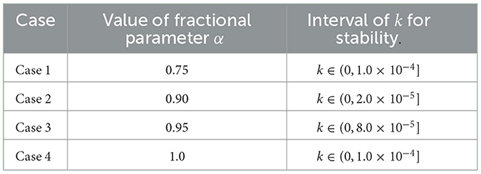
Table 1. Range of values of k for stability when $h=\frac{\pi }{64}$ at four different values of α using FTCSCO scheme.

We present the results using FTCSCO using k close to maximum k for stability and a lower value of k when $h=\frac{\pi }{64}$ in Figure 2.

Figure 2

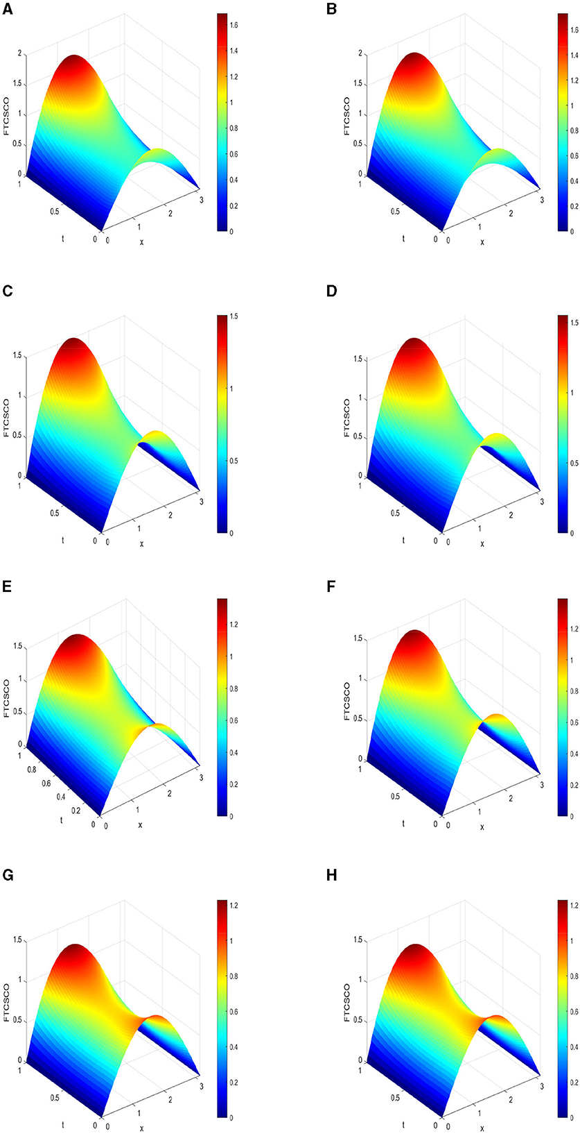
Figure 2. 3D plots of numerical solution vs. x∈[0, π] vs. t∈[0, 1] using FTCSCO scheme at $h=\frac{\pi }{64}$. (A) α = 0.75, k = 1.0 × 10⁻⁴. (B) α = 0.75, k = 1.0 × 10⁻⁵. (C) α = 0.90, k = 2.0 × 10⁻⁵. (D) α = 0.90, k = 2.0 × 10⁻⁶. (E) α = 0.95, k = 5.0 × 10⁻⁵. (F) α = 0.95, k = 5.0 × 10⁻⁶. (G) α = 1.0, k = 1.0 × 10⁻⁴. (H) α = 1.0, k = 1.0 × 10⁻⁵.

Figure 3

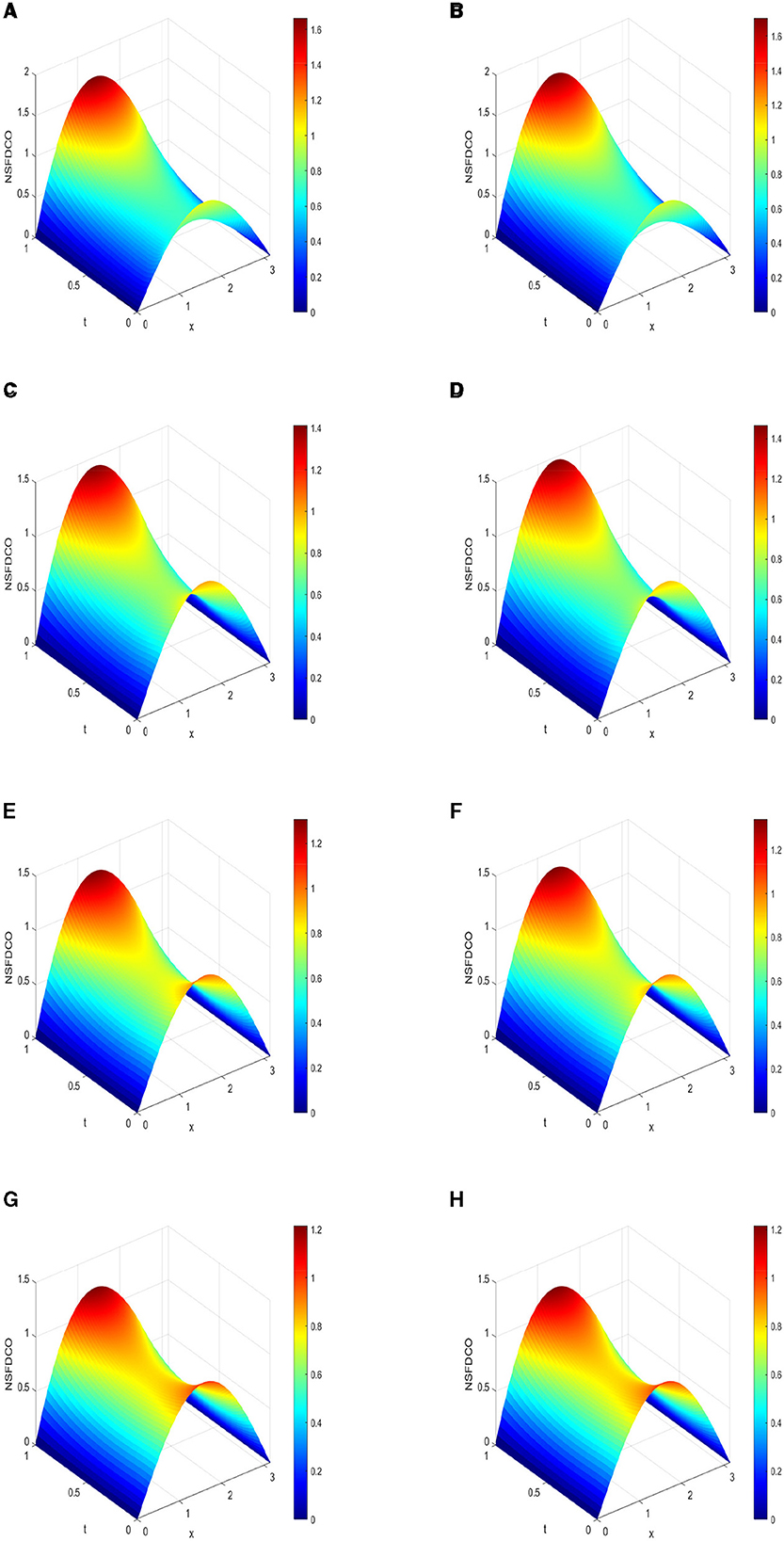
Figure 3. 3D plots of numerical solution vs. x∈[0, π] vs. t∈[0, 1] using NSFDCO scheme. (A) α = 0.75, k = 1.0 × 10⁻⁴. (B) α = 0.75, k = 1.0 × 10⁻⁵. (C) α = 0.90, k = 5.0 × 10⁻⁴. (D) α = 0.90, k = 5.0 × 10⁻⁵. (E) α = 0.95, k = 8.0 × 10⁻⁴. (F) α = 0.95, k = 8.0 × 10⁻⁵. (G) α = 1.0, k = 1.0 × 10⁻³. (H) α = 1.0, k = 1.0 × 10⁻⁴.

4.3 Consistency of the FTCSCO scheme

We consider Equation 18 and obtain Taylor's series expansion about (t_n, x_i). This gives

$\begin{array}{l}U+k{U}_t+\frac{k^2}{2}{U}_{tt}+\frac{k^3}{6}{U}_{ttt}+\mathcal{O}(k^4)+(1+x_i)U{k}^{\alpha }\\ =U+\frac{k^{\alpha }}{h^2}[(U+h{U}_x+\frac{h^2}{2!}{U}_{xx}+\frac{h^3}{3!}{U}_{xxx}+\frac{h^4}{4!}{U}_{xxxx}+\mathcal{O}(h^5))\\ -2U+(U-h{U}_x+\frac{h^2}{2!}{U}_{xx}-\frac{h^3}{3!}{U}_{xxx}+\frac{h^4}{4!}{U}_{xxxx}+\mathcal{O}(h^5))]\\ +k^{\alpha }·[x_i\left(\pi -x_i\right)\left(1+t_n^4\right)+t_n^2],\end{array}$

which gives

$\begin{array}{l}k{U}_t+\frac{k^2}{2}{U}_{tt}+\mathcal{O}(k^3)=\frac{k^{\alpha }}{h^2}[h^2{U}_{xx}+\frac{2h^4}{4!}{U}_{xxxx}+\mathcal{O}(h^6)]\\ +k^{\alpha }·[x_i\left(\pi -x_i\right)\left(1+t_n^4\right)+t_n^2]-(1+x_i)·U·k^{\alpha }.& (21)\end{array}$

If we multiply both sides of Equation 21 by k^−α, we obtain Equation 22

$\begin{array}{l}{k}^{1-\alpha }{U}_t+\frac{k^{2-\alpha }}{2}{U}_{tt}+\mathcal{O}\left(k^{3-\alpha }\right)=\frac{1}{h^2}[h^2{U}_{xx}+\frac{h^4}{12}{U}_{xxx}+\mathcal{O}\left(h^6\right)]\\ +[x_i\left(\pi -x_i\right)\left(1+t_n^4\right)+t_n^2]-(1+x_i)·U.& (22)\end{array}$

Since $\frac{{\partial }^{\alpha }U(x,t)}{\partial t^{\alpha }}\simeq k^{1-\alpha }\frac{\partial U}{\partial t}$, we therefore rewrite Equation 22 as Equation 23:

$\begin{array}{l}\frac{{\partial }^{\alpha }U}{\partial t^{\alpha }}=\frac{{\partial }^{2}U}{\partial x^2}-(1+x)U+\left(x\left(\pi -x\right)\left(1+t^4\right)+t^2\right)\\ +\mathcal{O}\left(h^2\right)+\mathcal{O}\left(k^{2-\alpha }\right).& (23)\end{array}$

Thus, FTCSCO scheme is consistent with the PDE given by Equation 6 and is accurate of order (2−α) in time and of order 2 in space, respectively.. For α = 0.75, 0.90, 0.95, and 1.0, the theoretical rates of convergence in time of FTCSCO scheme are 1.25, 1.1, 1.05, and 1, respectively.

4.4 Numerical results using FTCSCO

Figure 2 illustrates 3D plots of the numerical solution vs. x for t∈[0, 1.0] at two values of time step sizes when $h=\frac{\pi }{64}$.

As we increase α, the peak of the numerical solution decreases. The profiles are different when α changes.

In the following section, we present a nonstandard finite difference scheme employing conformable derivatives. We tabulate the numerical rate of convergence in Tables 2–5. To ensure stability, we varied the value of k around the maximum for stability and opted for a lower value of k when $h=\frac{\pi }{64}$.

Table 2

Table 2. Numerical rate of convergence in time for the four schemes using α = 0.75 at time 1.0.

Table 3

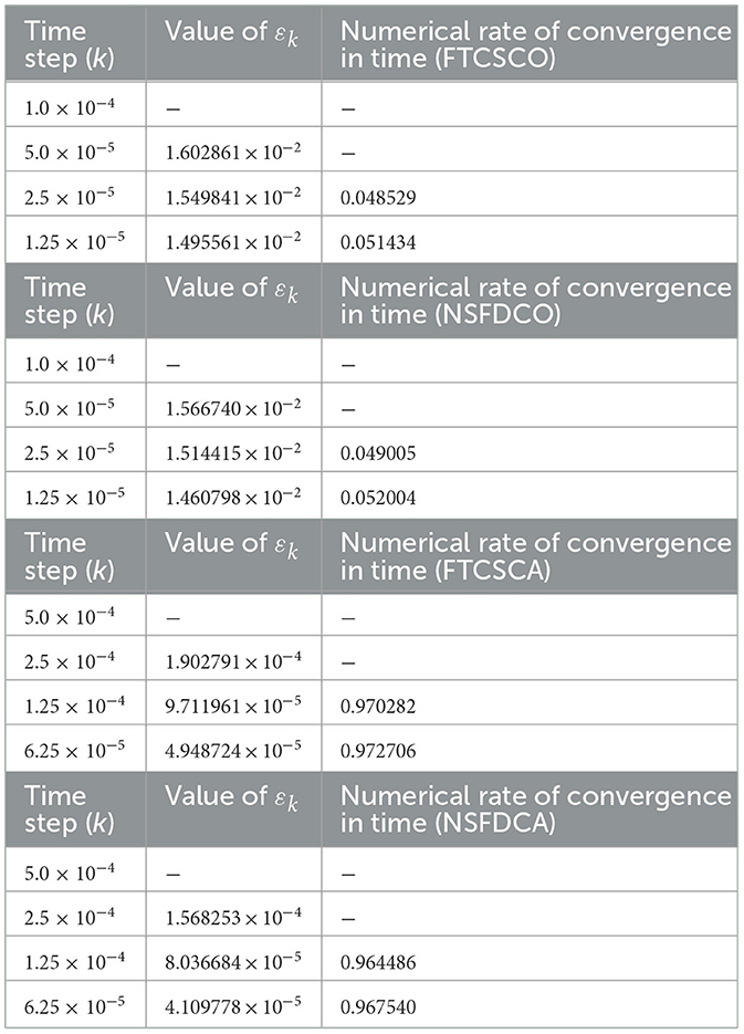
Table 3. Numerical rate of convergence in time for the four schemes using α = 0.90 at time 1.0.

Table 4

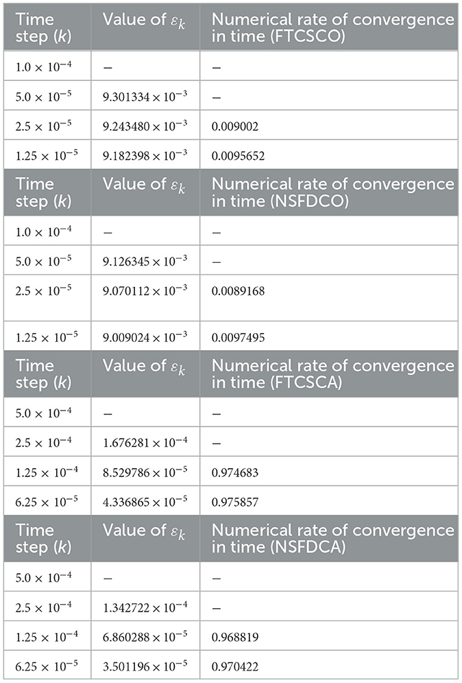
Table 4. Numerical rate of convergence in time for the four schemes using α = 0.95 at time 1.0.

Table 5

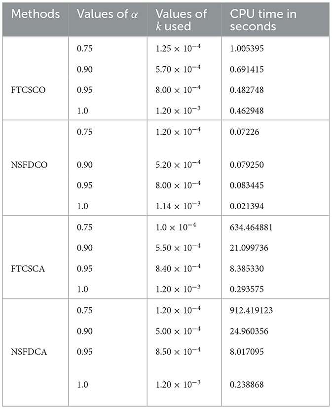
Table 5. Tabulation comparing the numerical schemes' CPU time at maximum possible value of k with $h=\frac{\pi }{64}$.

5 Nonstandard finite difference scheme using conformable operator (NSFDCO)

Mickens is the architect of nonstandard finite difference methods, and the rules for the construction of these methods are given in [21]. We construct a new scheme denoted as NSFDCO scheme. We first approximate the fractional derivative using conformable operators, and then, nonstandard finite difference approximations are used to approximate the derivatives. The NSFDCO scheme is given by

$\begin{array}{l}{k}^{1-\alpha }\left(\frac{U_i^{n+1}-U_i^n}{\varphi (k)}\right)-\frac{U_{i+1}^n-2U_i^n+U_{i-1}^n}{{\left(\psi (h)\right)}^2}\\ =(t_n{)}^2+x_i\left(\pi -x_i\right)\left(1+{(t_n)}^4\right)-(1+x_i)U_i^n,& (24)\end{array}$

where ϕ(k) = e^k−1 and ψ(h) = 1−e^−h.

By multiplying Equation 24 by ϕ(k)·k^α−1, we obtain Equation 25 and Equation 26

$\begin{array}{l}{U}_i^{n+1}=U_i^n-\left(\frac{\varphi (k)·k^{\alpha -1}}{{\left(1-e^{-h}\right)}^2}\right)(U_{i+1}^n-2U_i^n+U_{i-1}^n)\\ +(t_n{)}^2\varphi (k)·k^{\alpha -1}+\varphi (k)x_i\left(\pi -x_i\right)\left(1+{(t_n)}^4\right)·k^{\alpha -1}\\ -(1+x_i)·\varphi (k)·k^{\alpha -1}{U}_i^n.& (25)\end{array}$

$\begin{array}{l}{U}_i^{n+1}=[1-\frac{2\varphi (k)·k^{\alpha -1}}{{\left(1-e^{-h}\right)}^2}-(1+x_i)\varphi (k)·k^{\alpha -1}]U_i^n\\ +\left(\frac{\varphi (k)·{(k)}^{\alpha -1}}{{\left(1-e^{-h}\right)}^2}\right)(U_{i+1}^n+U_{i-1}^n)\\ +(t_n{)}^2\varphi (k)·(k{)}^{\alpha -1}+\varphi (k)x_i\left(\pi -x_i\right)\left(1+{(t_n)}^4\right)·(k{)}^{\alpha -1}.& (26)\end{array}$

5.1 Positivity condition of the NSFDCO scheme

We choose $h=\frac{\pi }{64}$. The range of k for NSFDCO to preserve positivity of solution of the continuous model must satisfy the inequality given by Equation 27:

$\begin{array}{ll}1-\frac{2\varphi (k)·{(k)}^{\alpha -1}}{{(1-e^{-h})}^2}-(1+x_i)\varphi (k)·k^{\alpha -1}\ge 0,& (27)\end{array}$

where ϕ(k) = e^k−1 and x_i∈[0, π].

Table 6 gives the range of values of k for which NSFDCO preserves positivity of solution of the continuous model when h is chosen as $\frac{\pi }{64}$.

Table 6

Table 6. Range of values of k for NSFDCO to be positivity preserving.

We note that for NSFD-based methods, the condition(s) for positivity is/are, in general, similar to condition(s) for stability [24].

5.2 Numerical results using NSFDCO

Since the numerical rate of convergence using FTCSCO and NSFDCO is not close to the theoretical rate of convergence for α = 0.75, 0.90, and 0.95 as depicted in Tables 2–4, we propose to construct other methods where fractional derivative are approximated by Caputo operators. We propose to construct FTCSCA and NSFDCA. FTCSCA is obtained by approximating fractional derivative using Caputo operators, and then, forward difference approximation is used for approximating $\frac{\partial u}{\partial t}$ and a central difference approximation is used for $\frac{{\partial }^{2}u}{\partial x^2}$.

6 Forward time central space scheme using caputo operator (FTCSCA)

6.1 Derivation of FTCSCA

To numerically solve Equation 6, we use an explicit forward in time and central in space finite difference scheme. We first approximate the time-fractional derivative using Caputo operators and then use forward difference approximations for $\frac{\partial u}{\partial t}$ and second-order central difference approximations for $\frac{{\partial }^{2}u}{\partial x^2}$.

Murio [51] derived an implicit scheme for a time-fractional diffusion equation. He approximated $\frac{{\partial }^{\alpha }u}{\partial t^{\alpha }}$ at the point (t_n, x_i) as follows:

$\begin{array}{l}\frac{{\partial }^{\alpha }u(x_i,t_n)}{\partial t^{\alpha }}=\frac{1}{\text{Γ}(1-\alpha )}{\displaystyle {\int }_0^{t_n}\frac{\partial u(x_i,t)}{\partial t}}\frac{1}{{\left(t_n-t\right)}^{\alpha }}\text{d}t\\ =\frac{1}{\text{Γ}(1-\alpha )}{\displaystyle \sum _{j=1}^n{\displaystyle {\int }_{(j-1)k}^{jk}\left[\frac{U_i^j-U_i^{j-1}}{k}+\Theta (k)\right]}}{\left(nk-t\right)}^{-\alpha }\text{d}t\\ =\frac{1}{\text{Γ}(1-\alpha )}{\displaystyle \sum _{j=1}^n\{}\left(\frac{U_i^j-U_i^{j-1}}{k}\right)[\frac{{(nk-t)}^{-\alpha +1}}{-(1-\alpha )}{]}_{t=(j-1)k}^{t=jk}\}\\ +\frac{1}{\text{Γ}(1-\alpha )}{\displaystyle \sum _{j=1}^n\{}[\frac{{(nk-t)}^{-\alpha +1}}{-(1-\alpha )}{]}_{t=(j-1)k}^{t=jk}\}·\Theta (k),\end{array}$

After some mathematical steps, it can be shown that [52]

$\begin{array}{l}\frac{{\partial }^{\alpha }u(x_i,t_n)}{\partial t^{\alpha }}\simeq \frac{k^{-\alpha }}{\text{Γ}(2-\alpha )}{\displaystyle \sum _{j=1}^n\{}\left(U_i^j-U_i^{j-1}\right)\\ ·[{\left(n-j+1\right)}^{1-\alpha }-{\left(n-j\right)}^{1-\alpha }]\}.\end{array}$

Appadu and Kelil [52] approximated $\frac{{\partial }^{\alpha }u(x_i,t_n)}{\partial t^{\alpha }}$ in a different way to Murio [51], and they obtained an explicit scheme in doing so. The authors in [52] approximated $\frac{{\partial }^{\alpha }u(x_i,t_n)}{\partial t^{\alpha }}$ as described briefly below.

$\begin{array}{l}\frac{{\partial }^{\alpha }u(x_i,t_n)}{\partial t^{\alpha }}\\ =\frac{1}{\text{Γ}(1-\alpha )}{\displaystyle \sum _{j=1}^n\{}{\displaystyle {\int }_{(j-1)k}^{jk}\left[\frac{U_i^{j+1}-U_i^j}{k}+\Theta (k)\right]}{\left(nk-\tau \right)}^{-\alpha }\text{d}\tau \}.\end{array}$

After some steps, they obtained [52]

$\begin{array}{l}\frac{{\partial }^{\alpha }u(x_i,t_n)}{\partial t^{\alpha }}\simeq \frac{1}{\text{Γ}(2-\alpha )}{k}^{-\alpha }{\displaystyle \sum _{j=1}^n\left(U_i^{j+1}-U_i^j\right)}.\\ [{\left(n-j+1\right)}^{1-\alpha }-{\left(n-j\right)}^{1-\alpha }].\\ =\frac{k^{-\alpha }}{\text{Γ}(2-\alpha )}\left(U_i^{n+1}-U_i^n\right)\\ +\frac{k^{-\alpha }}{\text{Γ}(2-\alpha )}\left\{{\displaystyle \sum _{j=1}^{n-1}\left(U_i^{n-j+1}-U_i^{n-j}\right)}\left[{(j+1)}^{1-\alpha }-j^{1-\alpha }\right]\right\}.& (28)\end{array}$

Using Equation 28, FTCSCA when used to discretize Equation 6 is given by

$\begin{array}{l}\frac{k^{-\alpha }}{\text{Γ}(2-\alpha )}\left(U_i^{n+1}-U_i^n\right)\\ +\frac{k^{-\alpha }}{\text{Γ}(2-\alpha )}{\displaystyle \sum _{j=1}^{n-1}\left(U_i^{n-j+1}-U_i^{n-j}\right)}\left[{(j+1)}^{1-\alpha }-j^{1-\alpha }\right]\}\\ -\frac{U_{i+1}^n-2U_i^n-U_{i-1}^n}{h^2}+(1+x_i)U_i^n\\ =x_i\left(\pi -x_i\right)\left(1+{(t_n)}^4\right)+(t_n{)}^2.& (29)\end{array}$

Multiplying Equation 29 by k^α Γ(2−α) gives

$\begin{array}{l}{U}_i^{n+1}-U_i^n+{\displaystyle \sum _{j=1}^{n-1}\left(U_i^{n+1-j}-U_i^{n-j}\right)}\left[{(j+1)}^{1-\alpha }-j^{1-\alpha }\right]\\ -k^{\alpha }\text{Γ}(2-\alpha )\left(\frac{U_{i+1}^n-2U_i^n+U_{i-1}^n}{h^2}\right)\\ +k^{\alpha }·\text{Γ}(2-\alpha )·(1+x_i)·U_i^n\\ =k^{\alpha }\text{Γ}(2-\alpha )x_i(\pi -x_i)[1+(t_n{)}^4]\\ +k^{\alpha }\text{Γ}(2-\alpha )(t_n{)}^2.& (30)\end{array}$

Equation 30 can be rewritten as

$\begin{array}{l}{U}_i^{n+1}=U_i^n-{\displaystyle \sum _{j=1}^{n-1}\left(U_i^{n+1-j}-U_i^{n-j}\right)}\left[{(j+1)}^{1-\alpha }-j^{1-\alpha }\right]\\ +k^{\alpha }\text{Γ}(2-\alpha )\left(\frac{U_{i+1}^n-2U_i^n+U_{i-1}^n}{h^2}\right)\\ -k^{\alpha }\text{Γ}(2-\alpha )(1+x_i)U_i^n\\ +k^{\alpha }\text{Γ}(2-\alpha )x_i(\pi -x_i)[1+(t_n{)}^4]\\ +k^{\alpha }\text{Γ}(2-\alpha )(t_n{)}^2.& (31)\end{array}$

Remark 1. For the case α = 1.0, we obtain the scheme given by Equation 32:

$\begin{array}{l}{U}_i^{n+1}=U_i^n+\frac{k}{h^2}\left(U_{i+1}^n-2U_i^n+U_{i-1}^n\right)-k(1+x_i)U_i^n\\ +k{x}_i(\pi -x_i)\left[1+{(t_n)}^4\right]+k(t_n{)}^2.& (32)\end{array}$

6.2 Stability of FTCSCA scheme

To study the stability, we consider the following scheme given by Equation 33:

$\begin{array}{l}{U}_i^{n+1}=U_i^n-{\displaystyle \sum _{j=1}^{n-1}\left(U_i^{n+1-j}-U_i^{n-j}\right)}\left[{(j+1)}^{1-\alpha }-j^{1-\alpha }\right]\\ +k^{\alpha }\text{Γ}(2-\alpha )\left(\frac{U_{i+1}^n-2U_i^n+U_{i-1}^n}{h^2}\right)\\ -k^{\alpha }\text{Γ}(2-\alpha )(1+x_i)U_i^n.& (33)\end{array}$

We substitute $U_i^n$ by ξⁿe^Iθih or ξⁿe^Iiω, where ω = θh, to obtain

$\begin{array}{l}{\xi }^{n+1}{e}^{Ii\omega }={\xi }^n{e}^{Ii\omega }-{\displaystyle \sum _{j=1}^{n-1}\left({\xi }^{n+1-j}-{\xi }^{n-j}\right)}\left[{(j+1)}^{1-\alpha }-j^{1-\alpha }\right]e^{Ii\omega }\\ +\frac{k^{\alpha }}{h^2}\text{Γ}(2-\alpha ){\xi }^n{e}^{Ii\omega }\left(e^{I\omega }-2+e^{-I\omega }\right)\\ -k^{\alpha }\text{Γ}(2-\alpha )(1+x_i){\xi }^n{e}^{Ii\omega }.& (34)\end{array}$

Dividing Equation 34 by e^Iiω, we obtain

$\begin{array}{l}{\xi }^{n+1}={\xi }^n-{\displaystyle \sum _{j=1}^{n-1}\left({\xi }^{n+1-j}-{\xi }^{n-j}\right)}\left[{(j+1)}^{1-\alpha }-j^{1-\alpha }\right]\\ +\frac{k^{\alpha }}{h^2}\text{Γ}(2-\alpha ){\xi }^n(2\cos (\omega )-2)\\ -k^{\alpha }\text{Γ}(2-\alpha )(1+x_i){\xi }^n.& (35)\end{array}$

On fixing n = 3 in Equation 35, we get Equation 36:

$\begin{array}{l}{\xi }^4={\xi }^3-{\displaystyle \sum _{j=1}^2\left({\xi }^{4-j}-{\xi }^{3-j}\right)}\left[{(j+1)}^{1-\alpha }-j^{1-\alpha }\right]\\ +\frac{k^{\alpha }}{h^2}\text{Γ}(2-\alpha ){\xi }^3(2\cos (\omega )-2)\\ -k^{\alpha }\text{Γ}(2-\alpha )(1+x_i){\xi }^3.& (36)\end{array}$

Case 1: We choose $h=\frac{\pi }{64}$ and α = 0.75 and obtain solutions for the amplification factor when $x_i=0,\frac{\pi }{4},\frac{\pi }{2},\frac{3\pi }{4},\pi$.

We have four solutions for ξ say ξ₁, ξ₂, ξ₃, and ξ₄ when x_i = 0. We then obtain 3D plots of |ξ₁| vs. k vs. ω∈[−π, π] and find range of k such that |ξ₁| ≤ 1.

We repeat the process with |ξ₂|, |ξ₃|, and |ξ₄|. For stability, we need |ξ₁| ≤ 1, |ξ₂| ≤ 1, |ξ₃| ≤ 1, |ξ₄| ≤ 1 and in that situation, we need 0 < k ≤ 0.000134.

We then change the value of x_i and repeat the same steps. We still obtain 0 < k ≤ 0.000134 for stability.

For the cases 2, 3, and 4, we change the value of the fractional parameter α and repeat the steps as done for Case 1 to obtain the range of k for stability.

We would like to point out that we could not work with a larger n as this cause the solution for the amplification factor to be too complicated and long. Moreover, Maple in that situation is not able to give explicit solutions for ξ when n>3.

6.3 Consistency of FTCSCA

We now rewrite the scheme in Equation 31 as

$\begin{array}{l}{U}_i^{n+1}=U_i^n-[(U_i^n-U_i^{n-1})(2^{1-\alpha }-1^{1-\alpha })\\ +(U_i^{n-1}-U_i^{n-2})(3^{1-\alpha }-2^{1-\alpha })\\ +(U_i^{n-2}-U_i^{n-3})(4^{1-\alpha }-3^{1-\alpha })+\dots +(U_i^2-U_i^1)\\ (n^{1-\alpha }-(n-1{)}^{1-\alpha })]\\ +\frac{k^{\alpha }}{h^2}\text{Γ}(2-\alpha )[U_{i+1}^n-2U_i^n+U_{i-1}^n]-k^{\alpha }\text{Γ}(2-\alpha )(1+x_i)U_i^n\\ +k^{\alpha }\text{Γ}(2-\alpha )x_i(\pi -x_i)[1+(t_n{)}^4]+k^{\alpha }\text{Γ}(2-\alpha )(t_n{)}^2.& (37)\end{array}$

Expanding Equation 37 using Taylor series expansion

$\begin{array}{l}U+k{U}_t+\frac{k^2}{2!}{U}_{tt}+\frac{k^3}{3!}{U}_{ttt}+\dots =U-\{\left[U-(U-k{U}_t+\frac{k^2}{2}{U}_{tt}-\frac{k^3}{6}{U}_{ttt}+\dots )\right](2^{1-\alpha }-1^{1-\alpha })\\ +\left[(U-k{U}_t+\frac{k^2}{2}{U}_{tt}-\frac{k^3}{6}{U}_{ttt}+\dots )-(U-2k{U}_t+\frac{{(2k)}^2}{2}{U}_{tt}-\frac{{(2k)}^3}{6}{U}_{ttt})\right](3^{1-\alpha }-2^{1-\alpha })\\ +\left[[U-2k{U}_t+\frac{{(2k)}^2}{2}{U}_{tt}-\frac{{(2k)}^3}{6}{U}_{ttt}]-(U-3k{U}_t+\frac{{(3k)}^2}{2}{U}_{tt}-\frac{{(3k)}^3}{6}{U}_{ttt})\right](4^{1-\alpha }-3^{1-\alpha })+\dots +\\ ([U-(n-2)k{U}_t+\frac{{((n-2)k)}^2}{2}{U}_{tt}-\frac{{((n-2)k)}^3}{6}{U}_{ttt}]-\\ [U-(n-1)k{U}_t+\frac{{((n-1)k)}^2}{2}{U}_{tt}-\frac{{((n-1)k)}^3}{6}{U}_{ttt}])(n^{1-\alpha }-(n-1{)}^{1-\alpha })\}+\\ \frac{k^{\alpha }}{h^2}\text{Γ}(2-\alpha )\left[U+h{U}_x+\frac{h^2}{2}{U}_{xx}+\frac{h^3}{6}{U}_{xxx}-2U+U-h{U}_x+\frac{h^2}{2}{U}_{xx}-\frac{h^3}{6}{U}_{xxx}\right]\\ -k^{\alpha }\text{Γ}(2-\alpha )(1+x_i)U+k^{\alpha }\text{Γ}(2-\alpha )x_i(\pi -x_i)(1+(t_n{)}^4)+k^{\alpha }\text{Γ}(2-\alpha )(t_n^2).& (38)\end{array}$

We simplify Equation 38 to get Equation 39:

$\begin{array}{l}U+k{U}_t+\frac{k^2}{2}{U}_{tt}+\frac{k^3}{6}{U}_{ttt}+\dots =U-\{(k{U}_t-\frac{k^2}{2}{U}_{tt}+\frac{k^3}{6}{U}_{ttt}+\dots )(2^{1-\alpha }-1^{1-\alpha })\\ +(k{U}_t-\frac{3k^2}{2}{U}_{tt}+\frac{7k^3}{6}{U}_{ttt}+\dots )(3^{1-\alpha }-2^{1-\alpha })\\ +(k{U}_t-\frac{5k^2}{2}{U}_{tt}+\frac{19k^3}{6}{U}_{ttt}+\dots )(4^{1-\alpha }-3^{1-\alpha })+\dots \\ +(k{U}_t-\frac{(2n-3)}{2}{U}_{tt}+\frac{3n^2-9n+7}{6}{U}_{ttt}+\dots )(n^{1-\alpha }-(n-1{)}^{1-\alpha })\}\\ +\frac{k^{\alpha }}{h^2}\text{Γ}(2-\alpha )(h^2{U}_{xx}+O(h^4))-k^{\alpha }\text{Γ}(2-\alpha )(1+x_i)U_i^n\\ +k^{\alpha }\text{Γ}(2-\alpha )x_i(\pi -x_i)(1+(t_n{)}^4)+k^{\alpha }\text{Γ}(2-\alpha )(t_n{)}^2.& (39)\end{array}$

Further simplification gives

$\begin{array}{l}k{U}_t+\frac{k^2}{2}{U}_{tt}+\frac{k^3}{6}{U}_{ttt}+\dots =-k{U}_t(n^{1-\alpha }-1^{1-\alpha })\\ -k^2{U}_{tt}\left(\frac{2^{1-\alpha }-1^{1-\alpha }}{2}+3\frac{3^{1-\alpha }-2^{1-\alpha }}{2}+\frac{5}{2}(4^{1-\alpha }-3^{1-\alpha })+\dots \right)\\ +\frac{k^{\alpha }}{h^2}\text{Γ}(2-\alpha )h^2{U}_{xx}+O(h^2{k}^{\alpha })-k^{\alpha }\text{Γ}(2-\alpha )(1+x_i)U_i^n\\ +k^{\alpha }\text{Γ}(2-\alpha )x_i(\pi -{\pi }_i)(1+(t_n{)}^4)+k^{\alpha }\text{Γ}(2-\alpha )(t_n{)}^2.& (40)\end{array}$

Dividing Equation 40 by Γ(2−α)k^α to get Equation 41:

$\begin{array}{l}{k}^{(1-\alpha )}{n}^{(1-\alpha )}{U}_t/\text{Γ}(2-\alpha )-U_{xx}+(1+x_i)U\\ =x_i(\pi -x_i)(1+(t_n{)}^4)+(t_n{)}^2+O(h^2)+O(k^{2-\alpha }).& (41)\end{array}$

Thus, the scheme is accurate of order 2 in space and of order (2−α) in time. We display profiles in Figure 4.

Figure 4

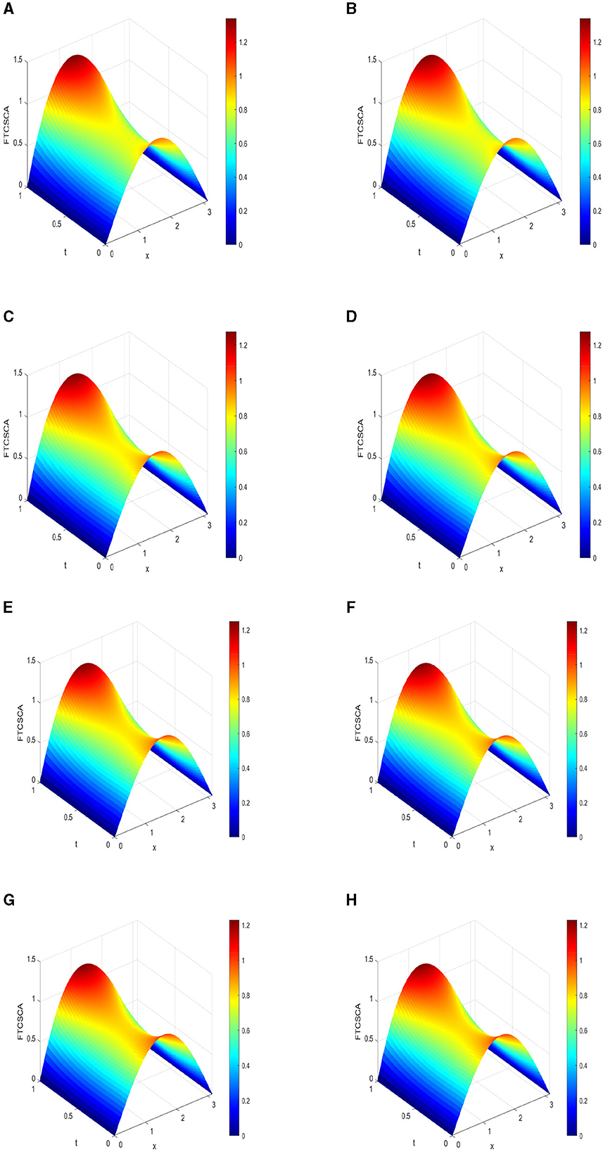
Figure 4. 3D plots of numerical solution vs. x∈[0, π] vs. t∈[0, 1] at $h=\frac{\pi }{64}$ using FTCSCA. (A) α = 0.75, k = 1.0 × 10⁻⁴. (B) α = 0.75, k = 5.0 × 10⁻⁵. (C) α = 0.90, k = 5.0 × 10⁻⁴. (D) α = 0.90, k = 5.0 × 10⁻⁵. (E) α = 0.95, k = 8.0 × 10⁻⁴. (F) α = 0.95, k = 8.0 × 10⁻⁵. (G) α = 1.0, k = 1.0 × 10⁻³. (H) α = 1.0, k = 1.0 × 10⁻⁴.

6.4 Numerical results using FTCSCA

The rate of convergence in time for FTCSCA displayed in Tables 2–4 (for α = 0.75. 0, 90, and 0.95 ) are close to the theoretical rate of convergence, hence a major advantage of FTCSCA over FTCSCO and NSFDCO. We therefore construct NSFDCA with hope that its numerical rate of convergence will also be close to theoretical one and that it will be easy to obtain condition for scheme to be positivity preserving as it is constructed using some nonstandard finite difference techniques.

7 Nonstandard finite difference scheme using caputo operator (NSFDCA)

7.1 Derivation of NSFDCA

We derive the nonstandard finite difference scheme where the fractional derivative is approximated by Caputo's operator, and then, nonstandard finite difference techniques are used to approximate $\frac{\partial u}{\partial t}$ and $\frac{{\partial }^{2}u}{\partial x^2}$.

We first obtain an approximation for $\frac{{\partial }^{\alpha }u(x_i,t_n)}{\partial t^{\alpha }}$ in Equation 42.

NSFDCA when used to discretize Equation 6 is given by Equation 43

$\begin{array}{l}\frac{{\partial }^{\alpha }u(x_i,t_n)}{\partial t^{\alpha }}=\frac{1}{\text{Γ}(1-\alpha )}{\displaystyle {\int }_0^{t_n}\frac{\partial u(x_i,\tau )}{\partial \tau }}(t_n-\tau {)}^{-\alpha }\text{d}\tau ,\text{ where }{t}_n=nk,\\ =\frac{1}{\text{Γ}(1-\alpha )}{\displaystyle \sum _{j=1}^n\{}{\displaystyle {\int }_{(j-1)k}^{jk}\left[\frac{U_i^{j+1}-U_i^j}{\varphi (k)}+\Theta (k)\right]}{\left(nk-\tau \right)}^{-\alpha }\text{d}\tau \}\\ =\frac{1}{\text{Γ}(1-\alpha )}{\displaystyle \sum _{j=1}^n\{}\left[\frac{U_i^{j+1}-U_i^j}{\varphi (k)}+\Theta (k)\right]{\displaystyle {\int }_{(j-1)k}^{jk}{\left(nk-\tau \right)}^{-\alpha }}\text{d}\tau \}\\ =\frac{1}{(1-\alpha )\text{Γ}(1-\alpha )}{\displaystyle \sum _{j=1}^n\{}\left(\frac{U_i^{j+1}-U_i^j}{\varphi (k)}+\Theta (k)\right)[-(nk-\tau {)}^{-\alpha +1}{]}_{\tau =(j-1)k}^{\tau =jk}\}\\ \simeq \frac{k^{1-\alpha }}{\text{Γ}(2-\alpha )}\left(\frac{U_i^{n+1}-U_i^n}{\varphi (k)}\right)\\ +\frac{k^{1-\alpha }}{\text{Γ}(2-\alpha )}{\displaystyle \sum _{j=1}^{n-1}\left(\frac{U_i^{j+1}-U_i^j}{\varphi (k)}\%+\Theta (k)\right)}·[{\left(n-j+1\right)}^{1-\alpha }-{\left(n-j\right)}^{1-\alpha }],\\ \simeq \frac{k^{1-\alpha }}{\text{Γ}(2-\alpha )}\frac{U_i^{n+1}-U_i^n}{\varphi (k)}\\ +\frac{k^{1-\alpha }}{\text{Γ}(2-\alpha )·\varphi (k)}{\displaystyle \sum _{j=1}^{n-1}\left(U_i^{j+1}-U_i^j\right)}·[{\left(n-j+1\right)}^{1-\alpha }-{\left(n-j\right)}^{1-\alpha }],\\ \simeq \frac{k^{1-\alpha }}{\text{Γ}(2-\alpha )}\frac{1}{\varphi (k)}\left(U_i^{n+1}-U_i^n\right)\\ +\frac{k^{1-\alpha }}{\varphi (k)}\frac{1}{\text{Γ}(2-\alpha )}{\displaystyle \sum _{j=1}^{n-1}\left(U_i^{n+1-j}-U_i^{n-j}\right)}·[{\left(j+1\right)}^{1-\alpha }-{\left(j\right)}^{1-\alpha }].& (42)\end{array}$

$\begin{array}{l}\frac{k^{1-\alpha }}{\varphi (k)}\frac{1}{\text{Γ}(2-\alpha )}\left(U_i^{n+1}-U_i^n\right)\\ +\frac{k^{1-\alpha }}{\varphi (k)}\frac{1}{\text{Γ}(2-\alpha )}{\displaystyle \sum _{j=1}^{n-1}\left(U_i^{n+1-j}-U_i^{n-j}\right)}\\ ·[{\left(j+1\right)}^{1-\alpha }-{\left(j\right)}^{1-\alpha }]\\ -\frac{U_{i+1}^n-2U_i^n+U_{i-1}^n}{{\left[\psi (h)\right]}^2}+(1+x_i)U_i^n\\ =x_i(\pi -x_i)(1+(t_n{)}^4)+(t_n{)}^2,& (43)\end{array}$

where ϕ(k) = e^k−1 and ψ(h) = 1−e^−h. Using Equation 43, we get Equation 44

$\begin{array}{l}{U}_i^{n+1}=U_i^n-{\displaystyle \sum _{j=1}^{n-1}\left(U_i^{n+1-j}-U_i^{n-j}\right)}·[{\left(j+1\right)}^{1-\alpha }-{\left(j\right)}^{1-\alpha }],\\ +\frac{\varphi (k)\text{Γ}(2-\alpha )}{k^{1-\alpha }}\left(\frac{U_{i+1}^n-2U_i^n+U_{i-1}^n}{{\left[\psi (h)\right]}^2}\right)\\ -\frac{\varphi (k)\text{Γ}(2-\alpha )}{k^{1-\alpha }}(1+x_i)U_i^n\\ +\frac{\varphi (k)\text{Γ}(2-\alpha )}{k^{1-\alpha }}{x}_i(\pi -x_i)\left[1+{(t_n)}^4\right]\\ +\frac{\varphi (k)\text{Γ}(2-\alpha )}{k^{1-\alpha }}(t_n{)}^2.& (44)\end{array}$

Remark 2. For α = 1.0, we obtain the scheme as

$\begin{array}{l}{U}_i^{n+1}=U_i^n+\varphi (k)\left(\frac{U_{i+1}^n-2U_i^n+U_{i-1}^n}{{\left[\psi (h)\right]}^2}\right)-\varphi (k)(1+x_i)U_i^n\\ +\varphi (k)x_i(\pi -x_i)\left[1+{(t_n)}^4\right]+\varphi (k)(t_n{)}^2.& (45)\end{array}$

7.2 Stability of NSFDCA scheme

To study the stability, we consider the following scheme given by Equation 46:

$\begin{array}{l}{U}_i^{n+1}=U_i^n-{\displaystyle \sum _{j=1}^{n-1}\left(U_i^{n+1-j}-U_i^{n-j}\right)}·[{\left(j+1\right)}^{1-\alpha }-{\left(j\right)}^{1-\alpha }]\\ +\frac{\varphi (k)\text{Γ}(2-\alpha )}{k^{1-\alpha }}\frac{U_{i+1}^n-2U_i^n+U_{i-1}^n}{{\left[\psi (h)\right]}^2}\\ -\frac{\varphi (k)\text{Γ}(2-\alpha )}{k^{1-\alpha }}(1+x_i)U_i^n.& (46)\end{array}$

We substitute $U_i^n$ by ξⁿe^Iθih or ξⁿe^Iiω, where ω = θh, to obtain Equation 47:

$\begin{array}{l}{\xi }^{n+1}{e}^{Ii\omega }={\xi }^n{e}^{Ii\omega }-e^{Ii\omega }{\displaystyle \sum _{j=1}^{n-1}\left({\xi }^{n+1-j}-{\xi }^{n-j}\right)}\left[{(j+1)}^{1-\alpha }-j^{1-\alpha }\right]\\ +\frac{\varphi (k)\text{Γ}(2-\alpha )}{k^{1-\alpha }}{\xi }^n{e}^{Ii\omega }\frac{\left(e^{I\omega }-2+e^{-I\omega }\right)}{{[\psi (h)]}^2}\\ -\frac{\varphi (k)}{k^{1-\alpha }}\text{Γ}(2-\alpha )(1+x_i){\xi }^n{e}^{Ii\omega }.& (47)\end{array}$

Dividing Equation 47 by e^Iiω, we obtain

$\begin{array}{l}{\xi }^{n+1}={\xi }^n-{\displaystyle \sum _{j=1}^{n-1}\left({\xi }^{n+1-j}-{\xi }^{n-j}\right)}\left[{(j+1)}^{1-\alpha }-j^{1-\alpha }\right]\\ +\frac{\varphi (k)}{k^{1-\alpha }}\text{Γ}(2-\alpha )\frac{{\xi }^n}{{[\psi (h)]}^2}\left(2\cos (\omega )-2\right)\\ -\frac{\varphi (k)}{k^{1-\alpha }}\text{Γ}(2-\alpha )(1+x_i){\xi }^n.& (48)\end{array}$

On fixing n = 3 in Equation 48, we Equation 49

$\begin{array}{l}{\xi }^4={\xi }^3-{\displaystyle \sum _{j=1}^2\left({\xi }^{4-j}-{\xi }^{3-j}\right)}\left[{(j+1)}^{1-\alpha }-j^{1-\alpha }\right]\\ +\frac{\varphi (k)\text{Γ}(2-\alpha )}{k^{1-\alpha }}\frac{{\xi }^2}{{[\psi (h)]}^2}\left(2\cos (\omega )-2\right)\\ -\frac{\varphi (k)\text{Γ}(2-\alpha )}{k^{1-\alpha }}(1+\pi ){\xi }^3.& (49)\end{array}$

Case 1: We choose $h=\frac{\pi }{64}$ and α = 0.75 and obtain solutions for the amplification factor when $x_i=0,\frac{\pi }{4},\frac{\pi }{2},\frac{3\pi }{4},\pi .$ We have 4 solutions for ξ, say ξ₁, ξ₂, ξ₃, ξ₄ when x_i = 0.

We then obtain 3D plots of |ξ₁| vs. k vs. ω∈[−π, π] and find the range of k such that |ξ₁| ≤ 1. We repeat the process with |ξ₂|, |ξ₃|, |ξ₄|.

For stability, we need |ξ₁| ≤ 1, |ξ₃| ≤ 1 , |ξ₄| ≤ 1 and for case 1, we have 10⁻⁷<k ≤ 1.25 × 10⁻⁴.

We then change the values of x_i and repeat the steps. We find that the range of vlaues of k for stability is unchanged; that is, 10⁻⁷<k ≤ 1.25 × 10⁻⁴.

Cases 2 and 3:

For these cases, we change the values of the fractional parameter and repeat the required steps to obtain range of values of k when $h=\frac{\pi }{64}$ for α = 0.90 and 0.95.

For case 4, we use scheme given by Equation 45 and obtain range of values of k for stability.

The results are summarized in Table 7.

Table 7

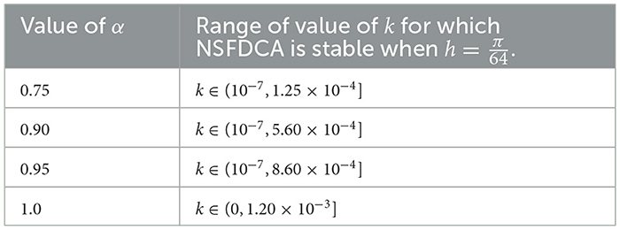
Table 7. Range of values of k for stability for the NSFDCA scheme at some fixed values of α when $h=\frac{\pi }{64}$.

7.3 Condition for positivity preserving

We consider the NSFDCA scheme, which is given by

$\begin{array}{l}{U}_i^{n+1}=\left[1-\frac{2\varphi (k)\text{Γ}(2-\alpha )}{k^{1-\alpha }{[\psi (h)]}^2}-\frac{\varphi (k)\text{Γ}(2-\alpha )(1+x_i)}{k^{1-\alpha }}\right]U_i^n+\left[\frac{\varphi (k)\text{Γ}(2-\alpha )}{k^{1-\alpha }{[\psi (h)]}^2}\right]U_{i+1}^n\\ +\left[\frac{\varphi (k)\text{Γ}(2-\alpha )}{k^{1-\alpha }{[\psi (h)]}^2}\right]U_{i-1}^n+\left[\frac{\varphi (k)\text{Γ}(2-\alpha )}{k^{1-\alpha }}\right](t_n{)}^2\\ +\left[\frac{\varphi (k)\text{Γ}(2-\alpha )}{k^{1-\alpha }}\right]x_i\left(\pi -x_i\right)\left[1+{(t_n)}^4\right]\\ -{\displaystyle \sum _{j=1}^{n-1}\left(U_i^{n+1-j}-U_i^{n-j}\right)}·[{\left(j+1\right)}^{1-\alpha }-{\left(j\right)}^{1-\alpha }].& (50)\end{array}$

We express

$\begin{array}{l}{\displaystyle \sum _{j=1}^{n-1}\left(U_i^{n+1-j}-U_i^{n-j}\right)}·[{\left(j+1\right)}^{1-\alpha }-{\left(j\right)}^{1-\alpha }]\\ =(U_i^n-U_i^{n-1})[2^{1-\alpha }-1^{1-\alpha }]+(U_i^{n-1}-U_i^{n-2})[3^{1-\alpha }-2^{1-\alpha }]\\ +(U_i^{n-2}-U_i^{n-3})[4^{1-\alpha }-3^{1-\alpha }]+\dots \\ +(U_i^3-U_i^2)((n-1{)}^{1-\alpha }+(U_i^2-U_i^1)(n^{1-\alpha }-(n-1{)}^{1-\alpha })\\ =U_i^n\left(2^{1-\alpha }-1\right)-U_i^{n-1}\left(2^{1-\alpha }-1\right)+U_i^{n-1}\left(3^{1-\alpha }-2^{1-\alpha }\right)-U_i^{n-2}\left(3^{1-\alpha }-2^{1-\alpha }\right)\\ +U_i^{n-2}\left(4^{1-\alpha }-3^{1-\alpha }\right)+U_i^{n-3}\left(4^{1-\alpha }-3^{1-\alpha }\right)+\mathrm{...}-U_i^2\left({(n-1)}^{1-\alpha }-{(n-2)}^{1-\alpha }\right)\\ +U_i^2\left(n^{1-\alpha }-{(n-1)}^{1-\alpha }\right)-U_i^1\left(n^{1-\alpha }-{(n-1)}^{1-\alpha }\right).& (51)\end{array}$

Using Equation 51, we rewrite Equation 50 as

We rewrite

$\begin{array}{l}{\displaystyle \sum _{j=1}^{n-1}\left(U_i^{n+1-j}-U_i^{n-j}\right)}·[{\left(j+1\right)}^{1-\alpha }-{\left(j\right)}^{1-\alpha }]\text{as}\\ U_i^n\left(2^{1-\alpha }-1\right)+U_i^{n-1}\left(3^{1-\alpha }-2·2^{1-\alpha }+1\right)\\ U_i^{n-2}\left(4^{1-\alpha }-2·3^{1-\alpha }+2^{1-\alpha }\right)\\ +\cdots +U_i^2(n^{1-\alpha }-2(n-1{)}^{1-\alpha }+(n-2{)}^{1-\alpha }).\end{array}$

Hence, the NSFDCA scheme from Equation 50 can be rewritten as

$\begin{array}{l}{U}_i^{n+1}=\left[1-\frac{2\varphi (k)\text{Γ}(2-\alpha )}{k^{1-\alpha }{[\psi (h)]}^2}-\frac{\varphi (k)\text{Γ}(2-\alpha )(1+x_i)+1-2^{1-\alpha }}{k^{1-\alpha }}\right]U_i^n\\ +\left[\frac{\varphi (k)\text{Γ}(2-\alpha )}{k^{1-\alpha }{[\psi (h)]}^2}\right]U_{i+1}^n+\left[\frac{\varphi (k)\text{Γ}(2-\alpha )}{k^{1-\alpha }{[\psi (h)]}^2}\right]U_{i-1}^n\\ +\left[\frac{\varphi (k)\text{Γ}(2-\alpha )}{k^{1-\alpha }}\right]x_i(\pi -x_i)\left[1+{(t_n)}^4\right]+\left[\frac{\varphi (k)\text{Γ}(2-\alpha )}{k^{1-\alpha }}\right](t_n{)}^2\\ +U_i^{n-1}\left(2·2^{1-\alpha }-3^{1-\alpha }-1\right)+U_i^{n-2}\left(2·3^{1-\alpha }-4^{1-\alpha }-2^{1-\alpha }\right)\\ ⋮\\ +U_i^2\left(2·{(n-1)}^{1-\alpha }-{(n)}^{1-\alpha }-{(n-2)}^{1-\alpha }\right).& (52)\end{array}$

From Equation 52, we find that the coefficients of $U_{i+1}^n$, $U_{i-1}^n$ and $U_i^{n-1}$, $U_i^{n-2}$, ⋯ , $U_i^2$ along with the expressions $\left[\frac{\varphi (k)\text{ Γ}(2-\alpha )}{k^{1-\alpha }}\right]x_i(\pi -x_i)\left[1+{(t_n)}^4\right]$, and $\left[\frac{\varphi (k)\text{ Γ}(2-\alpha )}{k^{1-\alpha }}\right]{(t_n)}^2$ are non-negative, using Maple software.

Hence, we require

$\begin{array}{l}1-\frac{2\varphi (k)\text{ Γ}(2-\alpha )}{k^{1-\alpha }{\left[\psi (h)\right]}^2}-\frac{\varphi (k)\text{ Γ}(2-\alpha )}{k^{1-\alpha }(1+x_i)}+1-2^{1-\alpha }\end{array}$

for the scheme to be positivity preserving. Table 8 gives range of values of k for scheme to be positivity preserving.

Table 8

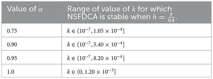
Table 8. Range of values of k for stability for the NSFDCA scheme at some fixed values of α when $h=\frac{\pi }{64}$.

7.4 Consistency of NSFDCA

To check the consistency of the NSFDCA scheme (Equation 45), we first need to rewrite the scheme as Equation 53:

$\begin{array}{l}{U}_i^{n+1}=U_i^n-{\displaystyle \sum _{j=1}^{n-1}\left(U_i^{n+1-j}-U_i^{n-j}\right)}·[{\left(j+1\right)}^{1-\alpha }-{\left(j\right)}^{1-\alpha }]\\ +\frac{\varphi (k)\text{Γ}(2-\alpha )}{k^{1-\alpha }}\left(\frac{U_{i+1}^n-2U_i^n+U_{i-1}^n}{{\left[\psi (h)\right]}^2}\right)\\ -\frac{\varphi (k)\text{Γ}(2-\alpha )}{k^{1-\alpha }}(1+x_i)U_i^n\\ +\frac{\varphi (k)\text{Γ}(2-\alpha )}{k^{1-\alpha }}{x}_i(\pi -x_i)\left[1+{(t_n)}^4\right]\\ +\frac{\varphi (k)\text{Γ}(2-\alpha )}{k^{1-\alpha }}(t_n{)}^2.& (53)\end{array}$

We can express this scheme as

$\begin{array}{l}{U}_i^{n+1}=U_i^n-(U_i^n-U_i^{n-1})[2^{1-\alpha }-1^{1-\alpha }]\\ +(U_i^{n-1}-U_i^{n-2})[3^{1-\alpha }-2^{1-\alpha }]\\ +(U_i^{n-2}-U_i^{n-3})[4^{1-\alpha }-3^{1-\alpha }]+\dots \\ +(U_i^2-U_i^1)(n^{1-\alpha }-(n-1{)}^{1-\alpha })\\ +\frac{\varphi (k)}{{[\psi (h)]}^2{k}^{1-\alpha }}\text{Γ}(2-\alpha )\left[U_{i+1}^n-2U_i^n+U_{i-1}^n\right]\\ -\frac{\varphi (k)\text{Γ}(2-\alpha )}{k^{1-\alpha }}(1+x_i)U_i^n\\ +\frac{\varphi (k)\text{Γ}(2-\alpha )}{k^{1-\alpha }}{x}_i(\pi -x_i)\left[1+{(t_n)}^4\right]\\ +\frac{\varphi (k)\text{Γ}(2-\alpha )}{k^{1-\alpha }}(t_n{)}^2.& (54)\end{array}$

By expanding Equation 54 using Taylor series, we obtain

$\begin{array}{l}U+k{U}_t+\frac{k^2}{2!}{U}_{tt}+\frac{k^3}{3!}{U}_{ttt}+\dots \\ =U-\left[(U-k{U}_t+\frac{k^2}{2!}{U}_{tt}-\frac{k^3}{3!}{U}_{ttt}+\dots )\right][2^{1-\alpha }-1^{1-\alpha }]\\ +[(U-k{U}_t+\frac{k^2}{2!}{U}_{tt}-\frac{k^3}{3!}{U}_{ttt}+\dots )\\ -(U-2k{U}_t+\frac{{(2k)}^2}{2!}{U}_{tt}-\frac{{(2k)}^3}{3!}{U}_{ttt}+)][3^{1-\alpha }-2^{1-\alpha }]\\ +[[U-2k{U}_t+\frac{{(2k)}^2}{2!}{U}_{tt}-\frac{{(2k)}^3}{3!}{U}_{ttt}]\\ -(U-3k{U}_t+\frac{{(3k)}^2}{2!}{U}_{tt}-\frac{{(3k)}^3}{3!}{U}_{ttt})][4^{1-\alpha }-3^{1-\alpha }]\\ +\frac{\varphi (k)}{{[\psi (h)]}^2{k}^{1-\alpha }}[U+h{U}_x+\frac{h^2}{2!}{U}_{xx}+\frac{h^3}{3!}{U}_{xxx}\\ -2U+U-h{U}_x+\frac{h^2}{2!}{U}_{xx}-\frac{h^3}{3!}{U}_{xxx}]\\ +\frac{\varphi (k)\text{Γ}(2-\alpha )}{k^{1-\alpha }}{x}_i(\pi -x_i)\left[1+{(t_n)}^4\right]+\frac{\varphi (k)\text{Γ}(2-\alpha )}{k^{1-\alpha }}(t_n{)}^2.& (55)\end{array}$

We simplify Equation 55 using the approximations ψ(h) = 1−e^−h≈h for small h, while retaining the function ϕ(k) = e^k−1≈k, which yields Equation 56 shown below:

$\begin{array}{l}U+k{U}_t+\frac{k^2}{2!}{U}_{tt}+\frac{k^3}{3!}{U}_{ttt}+\dots \\ =U-\left[(k{U}_t-\frac{k^2}{2}{U}_{tt}+\frac{k^3}{6}{U}_{ttt}+\dots )\right][2^{1-\alpha }-1^{1-\alpha }]\\ +\left[(k{U}_t-\frac{3k^2}{2}{U}_{tt}+\frac{7k^3}{6}{U}_{ttt}+\dots )\right][3^{1-\alpha }-2^{1-\alpha }]\\ +\left[(k{U}_t-\frac{5k^2}{2}{U}_{tt}+\frac{19k^3}{6}{U}_{ttt}+\dots )\right][4^{1-\alpha }-3^{1-\alpha }]\\ +\dots \\ +\left(k{U}_t-\frac{(2n-3)}{2}{U}_{tt}\mathrm{......}\right)(n^{1-\alpha }-(n-1{)}^{1-\alpha })\\ +\frac{k^{\alpha }}{h^2}\text{Γ}(2-\alpha )(h^2{U}_{xx}+O(h^4))-k^{\alpha }\text{Γ}(2-\alpha )(1+x_i)U_i^n\\ +k^{\alpha }\text{Γ}(2-\alpha )x_i(\pi -{\pi }_i)(1+(t_n{)}^4)+k^{\alpha }\text{Γ}(2-\alpha )(t_n{)}^2.& (56)\end{array}$

Further simplification gives

$\begin{array}{l}k{U}_t+\frac{k^2}{2!}{U}_{tt}+\frac{k^3}{3!}{U}_{ttt}+\dots =-k{U}_t(n^{1-\alpha }-1^{1-\alpha })\\ +k^2{U}_{tt}(\frac{2^{1-\alpha }-1^{1-\alpha }}{2}+3\frac{3^{1-\alpha }-2^{1-\alpha }}{2}\\ +\frac{5}{2}(4^{1-\alpha }-3^{1-\alpha })+\mathrm{...})\\ +\frac{k^{\alpha }}{h^2}\text{Γ}(2-\alpha )h^2{U}_{xx}+O(h^2{k}^{\alpha })-k^{\alpha }\text{Γ}(2-\alpha )(1+x_i)U_i^n\\ +k^{\alpha }\text{Γ}(2-\alpha )x_i(\pi -{\pi }_i)(1+(t_n{)}^4)+k^{\alpha }\text{Γ}(2-\alpha )(t_n{)}^2.& (57)\end{array}$

Dividing Equation 57 by Γ(2−α)k^α−1ϕ(k), we obtain Equation 58

$\begin{array}{l}\frac{n^{1-\alpha }{k}^{1-\alpha }}{\text{Γ}(2-\alpha )}{U}_t^{\alpha }-U_{xx}+(1+x_i)U=x_i(\pi -{\pi }_i)(1+(t_n{)}^4)\\ +(t_n{)}^2+O(h^2)+O(k^{2-\alpha }).& (58)\end{array}$

Thus, the NSFDCA scheme is accurate of order 2 in space and of order (2−α) in time. We also point out that the idea to prove consistency for both Caputo-based schemes shares a similar approach.

7.5 Numerical results using NSFDCA

The results using NSFDCA are displayed in Figure 5.

Figure 5

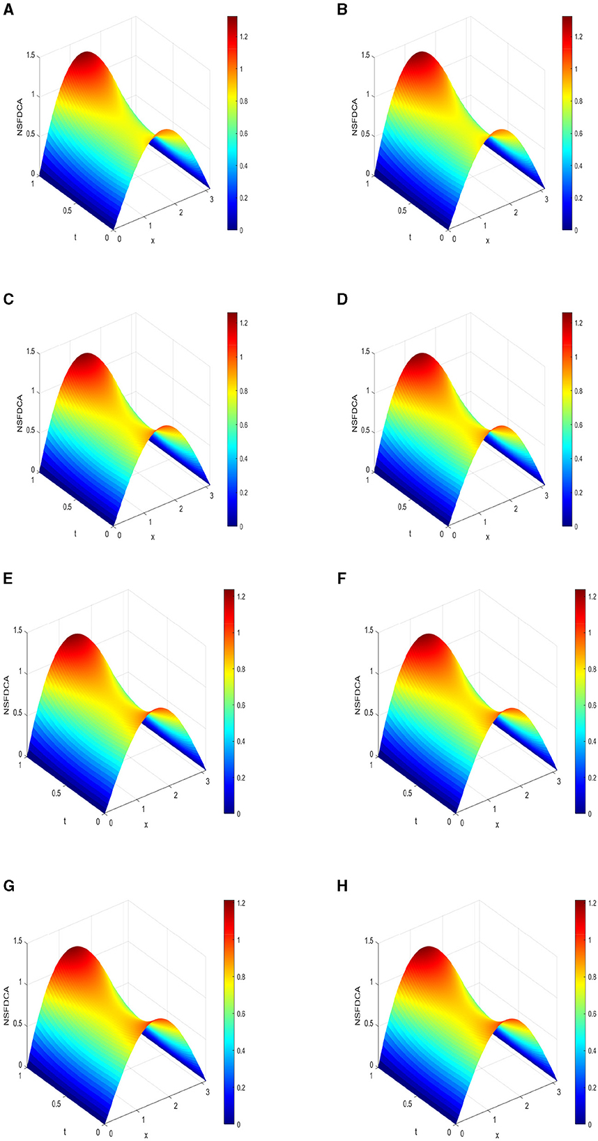
Figure 5. 3D plots of numerical solution using NSFDCA vs. x∈[0, π] vs. t∈[0, 1] with $h=\frac{\pi }{64}$. (A) α = 0.75, k = 1.0 × 10⁻⁴. (B) α = 0.75, k = 5.0 × 10⁻⁵. (C) α = 0.90, k = 5.0 × 10⁻⁴. (D) α = 0.90, k = 5.0 × 10⁻⁵. (E) α = 0.95, k = 8.0 × 10⁻⁴. (F) α = 0.95, k = 8.0 × 10⁻⁵. (G) α = 1.0, k = 1.0 × 10⁻³. (H) α = 1.0, k = 1.0 × 10⁻⁴.

8 Numerical rate of convergence for the four schemes.

8.1 Discussion of results

Figures 2–5 present 3D plots of of numerical solutions using FTCSCO, NSFDCO, FTCSCA, and NSFDCA schemes. These figures illustrate the variations across the spatial domain x∈[0, π] and time interval, namely, t∈[0, 1], respectively.

Tables 1, 6, 7, and 9 gives the range of values of k for stability using FTCSCO, NSFDCO, FTCSCA, and NSFDCA schemes when $h=\frac{\pi }{64}$.

Table 9

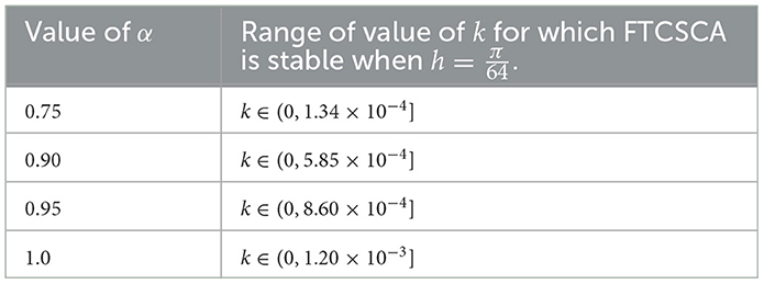
Table 9. Range of values of k for stability of FTCSCA when $h=\frac{\pi }{64}$ at four different values of α.

Remark 3. We note that for α = 0.75, the FTCSCO and NSFDCO methods exhibit remarkably similar convergence rates, affirming the robustness of these approaches. However, the FTCSCA and NSFDCA methods demand significantly more computational time to determine the temporal rate of convergence at α = 0.75 and t = 1.0. This heightened computational requirement likely stems from the intricate summative expressions employed to approximate the Caputo fractional derivative in both the FTCSCA and NSFDCA schemes.

Table 3 shows the temporal numerical rate of convergence obtained from the four numerical methods using $h=\frac{\pi }{64}$ and α = 0.90, whereas Table 4 illustrates the numerical rate of convergence when α = 0.95.

Table 5 presents a comparison of computational times at the maximum value of k for stability with a step size of $h=\frac{\pi }{64}$. It is pertinent to note that in each scenario, the iteration count is precisely maintained as an integer.

Our findings indicate a markedly quicker computational performance of the NSFDCO scheme in comparison with the FTCSCO, under identical conditions of k and h. The NSFDCA and FTCSCA schemes demonstrate approximately equivalent CPU times for the same parameter configurations.

Furthermore, the analysis conducted on the numerical rate of convergence reveals a closely matched performance between the FTCSCO and NSFDCO schemes, a pattern that is echoed in the comparison between NSFDCA and FTCSCA.

9 Conclusion

In this study, we have constructed four methods, namely, FTCSCO, FTCSCA, NSFDCO, and NSFDCA, to solve a time-fractional diffusion partial differential equation with specified initial and boundary conditions, and considered five different values for the fractional parameter. Analyses of stability and consistency of the methods were done, and CPU times were computed. Numerical profiles vs. x vs. t were displayed. The numerical results obtained from these different schemes provide valuable insights into their performance and convergence behavior.

From the analysis of NSFDCO, we conclude that it offers an easily obtainable condition for positivity with significantly lower CPU time compared to FTCSCO. While both schemes exhibit similar profiles, for smaller coefficients of U_xx, FTCSCO may introduce dispersive oscillations and potential blow-up.

FTCSCA, utilizing previous time levels Caputo operator, provides a more accurate representation of non-local and history-dependent diffusion processes. Although stability is somehow not easy, with n = 3, we identified an approximate stability range for k at $h=\frac{\pi }{64}$. However, due to the complexity of ξ, explicit solution beyond n = 3 remains elusive. That is, it is not possible to use n>3 due to ξ being very complex and long expression for ξ and Maple cannot solve explicitly for ξ.

NSFDCA, focusing on stability and preserving the positivity of solutions, demonstrates comparable CPU times to FTCSCA for α close to 1.0. It is anticipated to exhibit less susceptibility to non-physical oscillations than FTCSCA, particularly for small coefficients of dissipation and stiff problems.

We note that dispersion analysis of explicit finite difference methods discretizing fractional partial differential equations using conformable and Caputo approximations is not straightforward as conformable approximation involves an approximation and hence a source of error. Moreover, the amplification factor gets very complicated when we construct an explicit FDM with Caputo approximation.

In our future study, we will delve into scenarios involving coefficients of dissipation much smaller than 1, obtaining solution for which intila profiles is still, pattern formations in coral reefs, and employing alternative operators to approximate fractional derivatives. These endeavors aim to further enhance our understanding and application of fractional diffusion schemes in diverse scientific contexts.

Data availability statement

The raw data supporting the conclusions of this article will be made available by the authors, without undue reservation.

Author contributions

AA: Conceptualization, Data curation, Formal analysis, Investigation, Methodology, Project administration, Resources, Software, Supervision, Validation, Visualization, Writing – original draft, Writing – review & editing. AK: Data curation, Formal analysis, Investigation, Methodology, Resources, Software, Visualization, Writing – original draft, Writing – review & editing. NN: Data curation, Formal analysis, Investigation, Methodology, Resources, Software, Visualization, Writing – original draft, Writing – review & editing.

Funding

The author(s) declare financial support was received for the research, authorship, and/or publication of this article. AA is grateful to Nelson Mandela University, where the study was carried out. AK is grateful for postdoctoral research funding from NRF scarce skills fellowship under grant number 138521. NN is grateful to the department of Mathematics for partially funding his tuition fees at Nelson Mandela University in 2023.

Acknowledgments

The authors are very grateful to the few reviewers for providing constructive feedback which enabled them to significantly improve the initial version of this study.

Conflict of interest

The authors declare that the research was conducted in the absence of any commercial or financial relationships that could be construed as a potential conflict of interest.

Publisher's note

All claims expressed in this article are solely those of the authors and do not necessarily represent those of their affiliated organizations, or those of the publisher, the editors and the reviewers. Any product that may be evaluated in this article, or claim that may be made by its manufacturer, is not guaranteed or endorsed by the publisher.

References

1. Podlubny I. Fractional Differential Equations: An Introduction to Fractional Derivatives, Fractional Differential Equations, to Methods of Their Solution and Some of Their Applications. San Diego, CA: Academic Press (1998).

Google Scholar

2. Miller KS, Ross B. An Introduction to the Fractional Calculus and Fractional Differential Equations. New York, NY: John Wiley and Sons(1993).

Google Scholar

3. Oldham K, Spanier J. The Fractional Calculus Theory and Applications of Differentiation and Integration to Arbitrary Order. New York, NY: Academic Press (1974).

Google Scholar

4. Eriqat T, Oqielat MN, Al-Zhour Z, Khammash GS, El-Ajou A, Alrabaiah H. Exact and numerical solutions of higher-order fractional partial differential equations: a new analytical method and some applications. Pramana. (2022) 96:207. doi: 10.1007/s12043-022-02446-4

Crossref Full Text | Google Scholar

5. Podlubny I. Fractional Differential Equations, Mathematics in Science and Engineering. New York, NY: Academic Press (1999).

Google Scholar

6. Caputo M. Linear models of dissipation whose Q is almost frequency independent—II. Geophys J Int. (1967) 13:529–39. doi: 10.1111/j.1365-246X.1967.tb02303.x

Crossref Full Text | Google Scholar

7. Hashan M, Jahan LN, Imtiaz S, Hossain ME. Modelling of fluid flow through porous media using memory approach: a review. Math Comput Simul. (2020) 177:643–73. doi: 10.1016/j.matcom.2020.05.026

Crossref Full Text | Google Scholar

8. Mainardi F. Fractional Calculus and Waves in Linear Viscoelasticity: An Introduction to Mathematical Models. London: World Scientific Publishing Europe Ltd. (2022).

Google Scholar

9. Awadalla M, Alahmadi J, Cheneke KR, Qureshi S. Fractional optimal control model and bifurcation analysis of human syncytial respiratory virus transmission dynamics. Fract Fract. (2024) 8:44. doi: 10.3390/fractalfract8010044

Crossref Full Text | Google Scholar

10. Shaikh AA, Qureshi S. Comparative analysis of Riemann-liouville, Caputo-fabrizio, and Atangana-Baleanu integrals. J Appl Math Comp Mech. (2022) 21:8. doi: 10.17512/jamcm.2022.1.08

Crossref Full Text | Google Scholar

11. Li X, Wang H, Zhang Z, Hastings A. Mathematical analysis of coral reef models. J Math Anal Appl. (2014) 416:352–73. doi: 10.1016/j.jmaa.2014.02.053

Crossref Full Text | Google Scholar

12. Mistr S, Bercovici D. A theoretical model of pattern formation in coral reefs. Ecosystems. (2003) 6:0061–74. doi: 10.1007/s10021-002-0199-0

Crossref Full Text | Google Scholar

13. Wang RH, Liu QX, Sun GQ, Jin Z, van de Koppel J. Nonlinear dynamic and pattern bifurcations in a model for spatial patterns in young mussel beds. J R Soc Inter. (2009) 6:705–18. doi: 10.1098/rsif.2008.0439

PubMed Abstract | Crossref Full Text | Google Scholar

14. Somathilake LW, Burrage K. A space-fractional-reaction-diffusion model for pattern formation in coral reefs. Cogent Math Stat. (2018) 5:1426524. doi: 10.1080/23311835.2018.1426524

Crossref Full Text | Google Scholar

15. Gdawiec K, Argyros IK, Qureshi S, Soomro A. An optimal homotopy continuation method: Convergence and visual analysis. J Comput Sci. (2023) 74:102166. doi: 10.1016/j.jocs.2023.102166

Crossref Full Text | Google Scholar

16. Kelil AS, Appadu AR. On the numerical solution of 1D and 2D KdV equations using variational homotopy perturbation and finite difference methods. Mathematics. (2022) 10:4443. doi: 10.3390/math10234443

Crossref Full Text | Google Scholar

17. Jamali K, Solangi MA, Qureshi S. A novel hybrid iterative method for applied mathematical models with time-efficiency. J Appl Math Comp Mech. (2022) 21:2. doi: 10.17512/jamcm.2022.3.02

Crossref Full Text | Google Scholar

18. Qureshi S, Argyros IK, Soomro A, Gdawiec K, Shaikh AA, Hincal E. A new optimal root-finding iterative algorithm: local and semilocal analysis with polynomiography. Numer Alg. (2024) 95:1715–45. doi: 10.1007/s11075-023-01625-7

Crossref Full Text | Google Scholar

19. Qureshi S, Ramos H, Soomro AK, A. new nonlinear ninth-order root-finding method with error analysis and basins of attraction. Mathematics. (2021) 9:1996. doi: 10.3390/math9161996

Crossref Full Text | Google Scholar

20. Atangana A, Baleanu D. Numerical solution of a kind of fractional parabolic equations via two difference schemes. In: Abstract and Applied Analysis. Vol. 2013. Hindawi (2013). doi: 10.1155/2013/828764

Crossref Full Text | Google Scholar

21. Mickens RE. Applications of Nonstandard Finite Difference Schemes. Singapore: World Scientific (2000).

Google Scholar

22. Mickens RE. Dynamic consistency: a fundamental principle for constructing nonstandard finite difference schemes for differential equations. J Differ Eq Appl. (2005) 11:645–53. doi: 10.1080/10236190412331334527

Crossref Full Text | Google Scholar

23. Tijani YO, Appadu AR, Aderogba AA. Some finite difference methods to model biofilm growth and decay: classical and non-standard. Computation. (2021) 9:123. doi: 10.3390/computation9110123

Crossref Full Text | Google Scholar

24. Mickens R. An introduction to nonstandard finite difference schemes. J Comp Acoust. (2011) 11:07. doi: 10.1142/S0218396X99000059

PubMed Abstract | Crossref Full Text | Google Scholar

25. Momani S, Rqayiq AA, Baleanu D. A nonstandard finite difference scheme for two-sided space-fractional partial differential equations. Int J Bifur Chaos. (2012) 22:1250079. doi: 10.1142/S0218127412500794

Crossref Full Text | Google Scholar

26. Agbavon KM, Appadu AR. Construction and analysis of some nonstandard finite difference methods for the FitzHugh-Nagumo equation. Numer Methods Partial Differ Eq. (2020) 36:1145–69. doi: 10.1002/num.22468

Crossref Full Text | Google Scholar

27. Agarwal P, El-Sayed A. Non-standard finite difference and Chebyshev collocation methods for solving fractional diffusion equation. Phys A Stat Mech Appl. (2018) 500:40–9. doi: 10.1016/j.physa.2018.02.014

Crossref Full Text | Google Scholar

28. Tijani YO, Appadu AR. Unconditionally positive NSFD and classical finite difference schemes for biofilm formation on medical implant using Allen-Cahn equation. Demonstr Math. (2022) 55:40–60. doi: 10.1515/dema-2022-0006

Crossref Full Text | Google Scholar

29. Appadu AR, Tijani YO. 1D Generalised Burgers-Huxley: proposed solutions revisited and numerical solution using FTCS and NSFD methods. Front Appl Math Stat. (2022) 7:773733. doi: 10.3389/fams.2021.773733

Crossref Full Text | Google Scholar

30. Kehinde OO, Munyakazi JB, Appadu AR. A NSFD discretization of two-dimensional singularly perturbed semilinear convection-diffusion problems. Front Appl Math Stat. (2022) 8:861276. doi: 10.3389/fams.2022.861276

Crossref Full Text | Google Scholar

31. Jejeniwa OA, Gidey HH, Appadu AR. Numerical modeling of pollutant transport: results and optimal parameters. Symmetry. (2022) 14:2616. doi: 10.3390/sym14122616

Crossref Full Text | Google Scholar

32. Tarasov VE. Fractional Dynamics: Applications of Fractional Calculus to Dynamics of Particles, Fields and Media. Heidelberg: Springer (2011).

Google Scholar

33. Flekkøy EG, Hansen A, Baldelli B. Hyperballistic superdiffusion and explosive solutions to the non-linear diffusion equation. Front. Phys. (2021) 9:640560. doi: 10.3389/fphy.2021.640560

Crossref Full Text | Google Scholar

34. Metzler R, Klafter J. The random walk's guide to anomalous diffusion: a fractional dynamics approach. Phys Rep. (2000) 339:1–77. doi: 10.1016/S0370-1573(00)00070-3

Crossref Full Text | Google Scholar

35. Saichev AI, Zaslavsky GM. Fractional kinetic equations: solutions and applications. Chaos. (1997) 7:753–64. doi: 10.1063/1.166272

PubMed Abstract | Crossref Full Text | Google Scholar

36. Sokolov IM. Physics of Fractal Operators. American Institute of Physics. Physics Today. (2003) 56:65–6.

PubMed Abstract | Google Scholar

37. Stynes M, O'Riordan E, Gracia JL. Error analysis of a finite difference method on graded meshes for a time-fractional diffusion equation. SIAM J Numer Anal. (2017) 55:1057–79. doi: 10.1137/16M1082329

Crossref Full Text | Google Scholar

38. Bhatt HP, Khaliq AQM. Fourth-order compact schemes for the numerical simulation of coupled Burgers' equation. Comput Phys Commun. (2016) 200:117–38. doi: 10.1016/j.cpc.2015.11.007

Crossref Full Text | Google Scholar

39. Appadu AR, Waal GNd. Numerical solution of a malignant invasion model using some finite difference methods. Demonstratio Math. (2023) 56:20220244. doi: 10.1515/dema-2022-0244

Crossref Full Text | Google Scholar

40. Luchko Y. Some uniqueness and existence results for the initial-boundary-value problems for the generalized time-fractional diffusion equation. Comp Math Appl. (2010) 59:1766–72. doi: 10.1016/j.camwa.2009.08.015

Crossref Full Text | Google Scholar

41. Khalil R, Al Horani M, Yousef A, Sababheh M. A new definition of fractional derivative. J Comput Appl Math. (2014) 264:65–70. doi: 10.1016/j.cam.2014.01.002

Crossref Full Text | Google Scholar

42. Abdeljawad T. On conformable fractional calculus. J Comput Appl Math. (2015) 279:57–66. doi: 10.1016/j.cam.2014.10.016

Crossref Full Text | Google Scholar

43. Diethelm K, Ford NJ. Analysis of fractional differential equations. J Math Anal Appl. (2002) 265:229–48. doi: 10.1006/jmaa.2000.7194

Crossref Full Text | Google Scholar

44. Kilbas AA, Srivastava HM, Trujillo JJ. Theory and Applications of Fractional Differential Equations. Volume 204. Amsterdam: Elsevier (2006).

Google Scholar

45. Baleanu D, Diethelm K, Scalas E, Trujillo JJ. Fractional Calculus: Models and Numerical Methods. Volume 3. Singapore: World Scientific (2012).

Google Scholar

46. Nakagawa J, Sakamoto K, Yamamoto M. Overview to mathematical analysis for fractional diffusion equations: new mathematical aspects motivated by industrial collaboration. J. Math Indus. (2010) 2:99–108.

Google Scholar

47. Atangana A, Baleanu D, Alsaedi A. Analysis of time-fractional Hunter-Saxton equation: a model of neumatic liquid crystal. Open Phys. (2016) 14:145–9. doi: 10.1515/phys-2016-0010

Crossref Full Text | Google Scholar

48. Atangana A, Secer A. The time-fractional coupled-Korteweg-de-Vries equations. In: Abstract and Applied Analysis. Volume 2013. Hindawi (2013). doi: 10.1155/2013/947986

Crossref Full Text | Google Scholar

49. Strikwerda JC. Finite Difference Schemes and Partial Differential Equations. 2nd ed. Philadelphia, PA: SIAM (2004). 435 p.

Google Scholar

50. Hindmarsh A, Gresho P, Griffiths D. The stability of explicit Euler time-integration for certain finite difference approximations of the multi-dimensional advection-diffusion equation. Int J Numer Methods Fluids. (1984) 4:853–97. doi: 10.1002/fld.1650040905

Crossref Full Text | Google Scholar

51. Murio DA. Implicit finite difference approximation for time fractional diffusion equations. Comp Math Appl. (2008) 56:1138–45. doi: 10.1016/j.camwa.2008.02.015

Crossref Full Text | Google Scholar

52. Appadu AR, Kelil AS. Some Finite difference methods for solving linear fractional KdV equation. Front Appl Math Stat. (2023) 9:1261270. doi: 10.3389/fams.2023.1261270

Crossref Full Text | Google Scholar