 Ademe Kebede Gizaw*†
 Chernet Tuge Deressa†
- Department of Mathematics, College of Natural Sciences, Jimma University, Jimma, Ethiopia
Malaria remains a substantial public health challenge and economic burden globally. Currently, malaria has been declared as endemic in 85 countries. In this study, we developed and analyzed a fractional-order mathematical model for malaria transmission dynamics that incorporates variability of temperature and rainfall using Caputo-type AB operators. The existence and uniqueness of the model's solutions were established using the Banach fixed-point theorem. The model system's equilibria (both disease-free and endemic) were identified, and lemmas and theorems were developed to prove their stability. Furthermore, we used different temperature ranges and rainfall data, validating them against existing literature. Numerical simulations using the Toufik-Atangana schemes with various fractional-order alpha values revealed that as the value of alpha approaches 1, the behavior of the fractional-order model converges to that of the classical model. The numerical results are promising and are expected to be valuable for future research related to fractional-order models.
1 Introduction
Malaria, a life-threatening mosquito-borne disease, ranks among the deadliest infectious diseases worldwide [see [1] and references therein]. The World Health Organization (WHO) data for 2022 indicate ~249 million malaria cases, leading to 608,000 deaths in 85 countries [2]. This mosquito-borne infectious disease is the fifth leading cause of death from infectious diseases globally (after respiratory infections, HIV/AIDS, diarrheal diseases, and tuberculosis) and the second leading cause in Africa after HIV/AIDS [3]. Moreover, malaria remains a significant cause of mortality and morbidity in many tropical and subtropical regions, particularly within developing nations such as Ethiopia [see [4] and references therein].
In Ethiopia, with a population exceeding 120 million, more than 60% face the risk of contracting malaria [4]. This vulnerability stems from the fact that nearly 70% of Ethiopian land falls within areas suitable for malaria transmission, with altitude and rainfall serving as key risk factors.
Mathematical models of malaria transmission dynamics are valuable tools for understanding the disease, planning for the future, and implementing effective control measures [5]. The first integer-order model of this kind emerged from the study of Ross [6] and Macdonald [7]. While researchers have expanded these models over the years to incorporate various aspects of malaria transmission and control, research has given less attention to the impact of age structure. Recent studies have highlighted the significance of age structure in both the vector population and human population to understand the impact of climate variability on malaria transmission dynamics [see [8–10] and the references therein]. This is because environmental and climatic factors play a significant role in influencing the vector population's dynamics and the biting rate of mosquitoes on humans.
Temperature and rainfall are key drivers of mosquito population dynamics and subsequent malaria transmission, as reported in [11] and the references therein. These factors positively or negatively impact malaria transmission [12, 13]. Studies using real data from 67 sub-Saharan African cities have shown that the optimal temperature range for mosquito growth, and therefore malaria transmission, falls between 16 and 28°C [14]. This link between climate and malaria burden is further supported by data from South Africa's KwaZulu-Natal province [8]. Their findings reveal a clear trend: Within specific ranges, both increasing mean monthly temperature and rainfall are associated with increased malaria burden. Malaria burden rises with temperatures between 17 and 25°C and rainfall between 32 and 110 mm, while decreasing outside these ranges. Interestingly, Okuneye and Gumel [8] also pinpoints the specific temperature and rainfall combinations where malaria transmission peaks. Their data show that the highest transmission rates occur within the ranges of 21–25°C for temperature and 95–125 mm for rainfall. In addition to impacting transmission, temperature also directly affects the lifespan of adult female mosquitoes, which averages ~21 days [see [15] and the reference therein]. Notably, mosquito survival rapidly declines as temperatures exceed 34°C.
According to current literature and researchers' findings, all these models employ integer-order derivatives in their differential equations. However, fractional calculus has become increasingly prevalent in epidemic modeling [see [16–19] and as well some of the references therein]. This fractional approach has demonstrated significant advantages over integer-order modeling, offering a better fit to real data and possessing numerous other beneficial properties [20]. Furthermore, the memory and inheritance features of fractional calculus make it particularly well-suited for modeling and understanding real-world phenomena [20]. Within this framework, a variety of definitions and operators exist, including the Atangana–Baleanu [21], Caputo–Fabrizio [22], and Caputo derivatives [23], and serving as valuable tools for epidemic disease modeling.
Among these, the Caputo and Caputo–Fabrizio derivatives hold greater significance, with the latter particularly excelling due to its non-singular, non-local core and enhanced ability to reflect disease dynamics [[24] and the references within]. While the Atangana–Baleanu operator has found applications in modeling various real-world problems [24–28], its suitability for disease modeling specifically requires further evaluation.
Motivated by previous studies, we present a novel mathematical model of malaria transmission dynamics. Building upon the study of [8], our model analyzes and extends their framework by incorporating specific new compartments while omitting others. We further employ ABC fractional operators to explore the model's dynamics in a non-integer-order setting.
2 Mathematical preliminaries
This section presents important theorems and definitions of fractional calculus, especially some fundamental ideas about the Atangana–Baleanu fractional derivative operators and other related findings, before applying them to our suggested malaria model.
Definition 1. Let Ω ⊆ R be open and p ∈ [1;∞), so Hp(Ω) can be defined as
Definition 2. Yadeta et al. [29]. The Caputo derivative of fractional order p with n − 1 < p ≤ n; n ∈ N, for an integrable function g ∈ Cn, can be presented as
Definition 3. Atangana and Baleanu [21]. Let g ∈ H1(a, b), a < b, γ ∈ [0, 1], therefore, Atangana–Baleanu–Caputo (ABC) fractional derivative of g(t) with order γ is given by
where M(γ) is positive and is a normalization function fulfilling M(0) = M(1) = 1, and Eγ is the Mittag-Leffler function
where γ > 0 and z is complex number.
The Mittag-Leffler function with two parameters appears most frequently and has the following form:
Definition 4 Atangana and Baleanu [21]. Let g ∈ H1(a, b), a < b, γ ∈ [0, 1], then the Atangana–Baleanu Caputo integral of a function g(t) of order γ is defined by
Definition 5. Atangana and Baleanu [21]. The Laplace transform of the Atangana–Baleanu fractional derivative of order α in Caputo sense is given by
where is the Laplace transform operator.
Theorem 1. Atangana and Baleanu [21]. For a function g ∈ C[a, b], the inequality shown below holds.
where .
In addition, ABC derivatives satisfy the Lipschitz requirement; thus, we have
3 Model formulation
3.1 Presumptions of the model
The human population at time t, denoted by (Nh(t)), comprises two categories: adults and people under the age of seventeen. The latter group is further divided into susceptible children(Sc(t)), exposed children (Ec(t)), and infected children (Ic(t)). Adults are categorized into four compartments: susceptible (Sa(t)), exposed (Ea(t)), infected (Ia(t)), and recovered (Wa(t)). This leads to the following equation:
The total mosquito population at time t, denoted by (Nv(t)), is divided into immature (MA(t)) and mature mosquitoes (Mv(t)). Furthermore, there are three compartments in mature mosquitoes: susceptible mosquitoes (Sv(t)), exposed mosquitoes (Ev(t)), and infected mosquitoes (Iv(t)). So that:
In the compartmental model (12), πc is the recruitment rate for children, λi(T)(i = c, a, v) are the infection rate of susceptible children, adults, and vectors, respectively. bm(T) is the temperature-dependent per capital biting rate of mosquitoes, and βj(j = c, a, m) is the probability of infection per bite for children, adults, and mosquitoes. μh is the natural death rate of humans, and ξh is the maturation rate of children to adulthood. Immature mosquitoes (eggs, larvae, and pupae) are lumped into a single compartment (MA(t)) for computational convenience [see [8] and the references therein].
The temperature-dependent egg deposition rate is represented by αI(T). Following [14], we assume that the immature mosquito population (encompassing larvae and pupae) is limited by the carrying capacity Kv, where Kv exceeds MA. This parameter reflects the available nutrients and space, as detailed in [8] and its references. Therefore, represents the logistic growth rate for the immature mosquitoes.
Using the parameters and their definitions given in Tables 1, 2, we can write the model as a system of first-order ordinary differential equations:
where the infection rates for children (λc(T)), adults (λa(T)), and vectors (λv (T)) are given, respectively, by
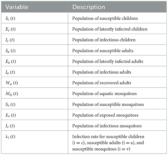
Table 1. Description of variables of the model (12).
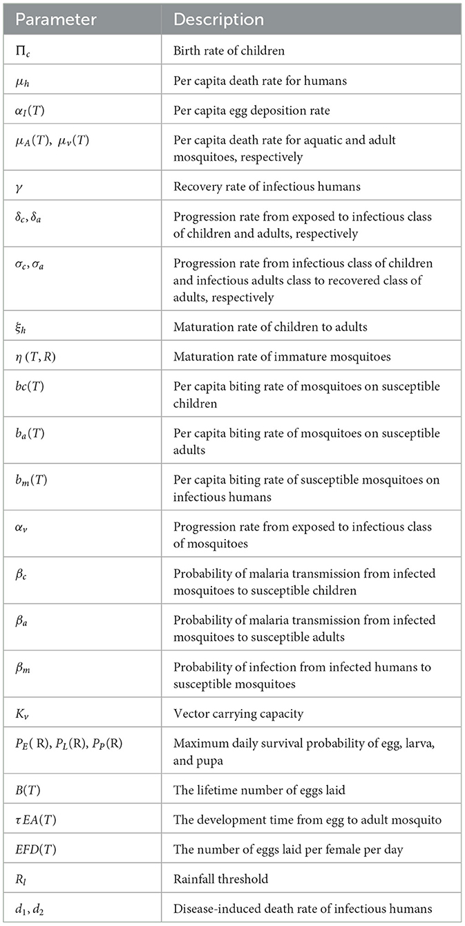
Table 2. Description of parameter of the model (12).
4 Model analysis
To account for long-term dependencies and complex memory effects in biological systems, we propose a fractional-order model for malaria. We replace the first-order ordinary derivatives in Equation 12—representing population change rates—with the Atangana–Baleanu fractional derivative of order α (0 < α ≤ 1) to incorporate internal memory effects.
with initial conditions:
where is Atangana-Beleanu in Caputo sense of order α, and the infection rates for children (λc(T)), adults (λa(T)), and vectors (λm (T)) are given, respectively, by
4.1 Existence and uniqueness of solutions
In this section, we will discuss the existence and uniqueness of solutions ABC fractional operators of the model system (13). To do this, we first re-write the model (13) in the following simple form:
In (17),
and F is a continuous vector function defined as
and
is the initial vector for state variables. The function F also satisfies the Lipschitz criterion, which is as follows:
where L is a Lipschitz constant.
The following lemma helps us to show the existence and uniqueness of the solution to the fractional model system (14):
Lemma 1. The unique solution of the differential equation with fractional order α is given by
is expressed as
Theorem 2. Under the condition that , then there exists a unique solution to the fractional-order malaria model (14).
Proof.
Let τ = (0, T), and the operator , as expressed in lemma (23), is given by
is expressed as
Furthermore, let:
where ||.||τ represents the supremum norm over τ.
Using Equation 25, we obtain:
From:
With:
u(x) ∈ C(τ, R11) and D(t, τ) ∈ C(τ2, R), that is:
Now, using Equations 28, 29 and the triangular inequality on Equation 27, we obtain
Therefore, we obtain
where
Hence, if L < 1 on , the operator becomes a contraction. Therefore, the fractional malaria model (14) has a unique solution by the Banach fixed-point theorem.
4.2 Positivity and boundedness of solutions
For the Atangana–Baleanu–Caputo fractional derivative models to be stable, have a steady state of existence, and have biological significance, their solutions have to be positive. Here is a lemma that can be used to prove the positivity of the solution to the proposed model.
Lemma 2. (Generalized Mean Value Theorem see [30]). Supposing that g(t) ∈ C[a, b] and for 0 < α ≤ 1, then
Remark 1 Suppose that g(t) ∈ C[0, b] and for 0 < α ≤ 1 from Lemma 2 one can deduce that
i. if , ∀t ∈ (0, b], then the function g(t) is non-decreasing and
ii. if , ∀t ∈ (0, b], then the function g(t) is non-increasing.
Theorem 3. The solution of the fractional malaria model (14)
which starts at, t = t0 remains in Ω for any t ≥ t0.
Proof. With reference [31], beginning with the first equation in Equation 14, we want to show that Sc(t) ≥ 0 for all t > t0.
If, to the contrary, it is not true, then there exists a constant t > t0 such that
Now, from the first equation in Equation 14 and based on Equation 38, we obtain
Consequently, invoking Remark 1 of lemma 2, we obtain , which contracts the assertion . Therefore, we conclude that Sc(t) ≥ 0 for all t > t0. Similarly, we establish the following inequalities for t > t0:
This completes the proofs of Theorem 3.
4.3 Invariant region
Given non-negative initial data, we identify the region where the solutions to the system of Equation 14 are viable. Here, we are primarily concerned with demonstrating that the viable region is located in , which is a positive invariant region with regard to the model (14) under the initial condition (15).
Theorem 4. Let the Atangana–Baleanu fractional model (14) has a unique solution (Nh, Nv) for all t ≥ 0. Then, the epidemiologically feasible region of the model is given by , where
and
Proof. Let Nh and Nv represent the total population of humans and mosquitoes, respectively. By adding all the equations corresponding to the human and mosquito components of the system (14), we get
and
To prove theorem 4, we need to show that system (14) has bounded solutions. Biologically, the least possible value of each state of the model system (14) is zero. Next, we determine the upper bound of the states. To do this,
let
and
Then, by applying the Laplace transform on both sides of Equation 44, we obtain
and using definition 5, we obtain
where Nh(0) represents the initial value of the total human population.
This implies that
Therefore,
Applying the inverse Laplace transform on both sides of (49), we get
where
Furthermore,
Thus,
since as t → ∞.
Thus, the epidemiologically feasible region for the human population is
Similarly, it can be shown that the feasible region for the mosquito population is
Thus, the proposed model is mathematically well-posed and epidemiologically sound on the region .
4.4 Existence of equilibrium points and the basic reproduction number
This section presents the disease-free and endemic equilibrium points of our Atangana–Baleanu fractional-order malaria model (14) to analyze their stability and dynamical behavior.
4.4.1 Disease-free equilibrium point
The steady-state solution of the model system (a form of the ABC fractional model) (14) obtained in the absence of disease is known as the disease-free equilibrium (DFE). The autonomous form of Equation 14 exhibits two disease-free equilibria, as stated in Theorem 6 below, depending on the magnitude of the threshold quantity M, where . For this analysis, we consider the special case of the non-autonomous version of model (14) in which the temperature- and rainfall-dependent parameters are constant, specifically: ηI(T, R) = ηI, αI(T) = αI, μA(T) = μA, and μv(T) = μv.
Theorem 5. The model system (14) possesses two malaria disease-free equilibrium points: the trivial disease-free equilibrium and the biologically realistic disease-free equilibrium . These equilibria are defined as follows:
• holds when .
• holds when .
where
Proof: To find the disease-free equilibria of the ABC fractional malaria model (14), we set the right-hand side of each equation in system (14) to zero and also set Ec = Ic = Ea = Ia = Ev = Iv = 0. This means all infected and infectious compartments are empty.
From the equations , we obtain two possibilities: either MA = 0 or .
Therefore:
i. : When MA = 0 and all infected and infectious compartments are empty (Ec = Ic = Ea = Ia = Ev = Iv = 0), and each equation in Equation 14 is equal to zero, we obtain
Therefore, .
ii. : When and all infected and infectious compartments are empty (Ec = Ic = Ea = Ia = Ev = Iv = 0), and each equation in Equation 14 is equal to zero, we obtain
Therefore, .
This completes the proof of Theorem 5.
4.4.2 The basic reproduction number
Definition 6. Diekmann et al. [32] and Van den Driessche and Watmough [33]. The basic reproductive number is the spectral radius (largest eigenvalue) of the next-generation matrix, where F represents the Jacobian of the rates of flows from uninfected to infected classes evaluated at the disease-free equilibrium and V is the Jacobian of the rates of all other flows to and from infected classes evaluated at the disease-free equilibrium.
Theorem 6.
i. If , then the basic reproduction number, R0, associated with system (14) is zero.
ii. If , then the basic reproduction number, R0, associated with system (14) is:
Proof. To compute the basic reproduction number of the ABC fractional malaria model (14) from the malaria disease-free equilibrium using the next-generation matrix method [33], we focus on the infected compartments (those representing disease progression dynamics) of the model, leading to the following subsystem:
Thus, the Jacobian matrix for the infected sub-population Equation 64 is given by
Now, we look at two cases to determine the basic production number.
Case I: Following (65), the transmission matrix F (of new infection terms) and the transition matrix V (of transition terms) corresponding to the fractional ABC model (14) at trivial disease-free equilibrium point () are given, respectively, by
and
where .
Thus,
The basic reproduction number in this particular case is zero because zero is the only eigenvalue of the matrix FV−1. This suggests that the disease will not spread if an infected person is introduced into the community at trivial disease-free site , that is, trivial disease-free site is locally asymptotically stable for this particular case.
Case II: Following (65), the transmission matrix F (of new infection terms) and the transition matrix V (of transition terms) associated with the fractional ABC model (14) at realistic disease-free equilibrium point are given, respectively, by
and
As a result, one can get
From (73), we get the characteristic polynomial
where
which implies that
Therefore,
where
This completes the proof of the Theorem 6.
Theorem 7. The malaria disease-free equilibrium points and are locally asymptotically stable if R0 < 1 and unstable if R0 > 1.
Proof. The Jacobian matrix is found about the malaria disease-free equilibrium:
where
The eigenvalues of Equation 79 are−(ξh + μh)−(δc + μh), −(μh + d1 + σc), −μh, −(μh + δa), −(σa + μh + d2), −(μh + γ), −(μv + αv), −μv, and have all negative real part, so for R0 < 1, the disease-free equilibrium is locally asymptotically stable.
The following Jacobian matrix is found about the biologically realistic disease-free equilibrium :
where
It follows from Equation 81, the eigenvalues −(ξh + μh), −μh, −(μh + γ), −(σa + μh + d2), −(μh + βa), and containing negative real parts. The remaining (four) eigenvalues are found in the roots of the equation provided below:
where the coefficients are
Thus, by Routh–Hurwitz criteria, the four eigenvalues found in the roots of will have a negative real part if they satisfy the Routh–Hurwitz criteria, that is, Ki > 0, for i = 1, ⋯ , 4.
It can be easily seen from the first, second, and third equations in Equation 84 that K1 > 0, K2 > 0, and K3 > 0, respectively.
Furthermore, from the fourth equation in Equation 84, we have
if R0 < 1 and K4 < 0, if R0 > 1.
Thus, for all 0 < α ≤ 1. Therefore, will be locally asymptotically stable for R0 < 1 and unstable for R0 > 1 as in [34].
Lemma. Vargas-De-León [35]. Let f(t) ∈ R+ be a continuous and differentiable function. Then, for any time instance t ≥ 0.
and
where 0 < α < 1.
Note that α = 1, the inequalities in Equations 86, 87 become equalities.
Theorem 8. If R0 < 1, then the malaria-free equilibria, and , of the proposed model (13) are global asymptotic stability.
Proof. To prove this, we construct a candidate Lyapunov function [36, 37] such that
where .
Now applying ABC operator on both sides of Equation 88, we get
Substituting Equation 14 into Equation 86 and after some algebraic simplification, we obtain
As
we conclude that
As a result, when 0 < α < 1 and if and only if . Thus, by LaSalle's invariance principle [38], the malaria-free equilibria, and , are globally asymptotically stable.
4.5 Existence of endemic equilibrium
The endemic equilibrium point of the fractional model (14), denoted by
, is defined where d1 = d2 = 0, which leads to, . This equilibrium point satisfies the following equation:
Accordingly, the roots of Equation 93 that are either 0 correspond to the disease-free equilibrium point or the non-zero roots of
where
Theorem 9. The endemic equilibrium of the model system (13) is globally asymptotically stable in Ω if R0 > 1.
Proof. To prove this, we define the Lyapunov function as follows:
L is continuously differentiable function and also
and applying lemma[35], we obtain
Applying Equation 14 from Equation 98, we obtain
By further rewriting this inequality, we have
This inequality can be rewritten as
where
and
As a result, for C1 < C2 and if and only if and . The largest closed and bounded invariant set in {: is the singleton {E*}, where E* is the endemic equilibrium point. As a result, when R0 > 1 in the region Ω, the unique equilibrium point E* is globally asymptotically stable, according to the LaSalle invariance principle [38]. This completes the proof of the theorem.
5 Sensitivity analysis
To ensure model predictions remain reliable despite potential uncertainties in parameter values, sensitivity analysis is widely conducted. It reveals how changes in parameters affect the system's overall dynamics, particularly in relation to the basic reproduction number, offering crucial insights. Sensitivity analysis using the fixed-point estimation method described in reference [39] is applied to the fractional malaria model (14). This method analyzes the effects of local changes in model parameters by calculating the normalized forward sensitivity index of a variable v to a parameter (p), which is defined as
We created Table 3 using the following values: bm = 0.29, δc = 0.0003, βm = 0.022, μh = 0.00005, πc = 540, η = 0.343, d1 = 0.0002, μA = 0.1041, αI = 1.84, ξh = 0.000161, and μv = 0.05 per day, Kv = 40000, αv = 0.5, and σc = 0.002 as given in [[8] and the references therein]. Figure 1 illustrates a schematic of the mathematical model for malaria transmission (Equation 12), based on the works of [8, 10].
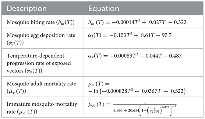

Figure 1. A schematic of the mathematical model for malaria transmission.
Figure 2 depicts the sensitivity analysis of the basic reproduction number [fractional malaria model (14)] for the 14 parameters in Table 4.
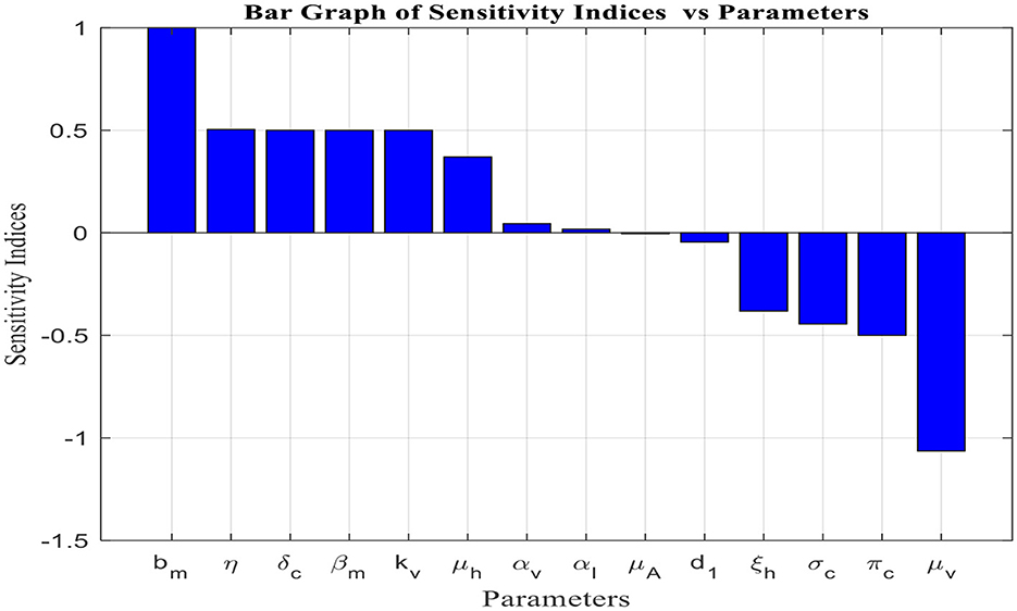
Figure 2. Sensitivity to model parameters (Table 2).
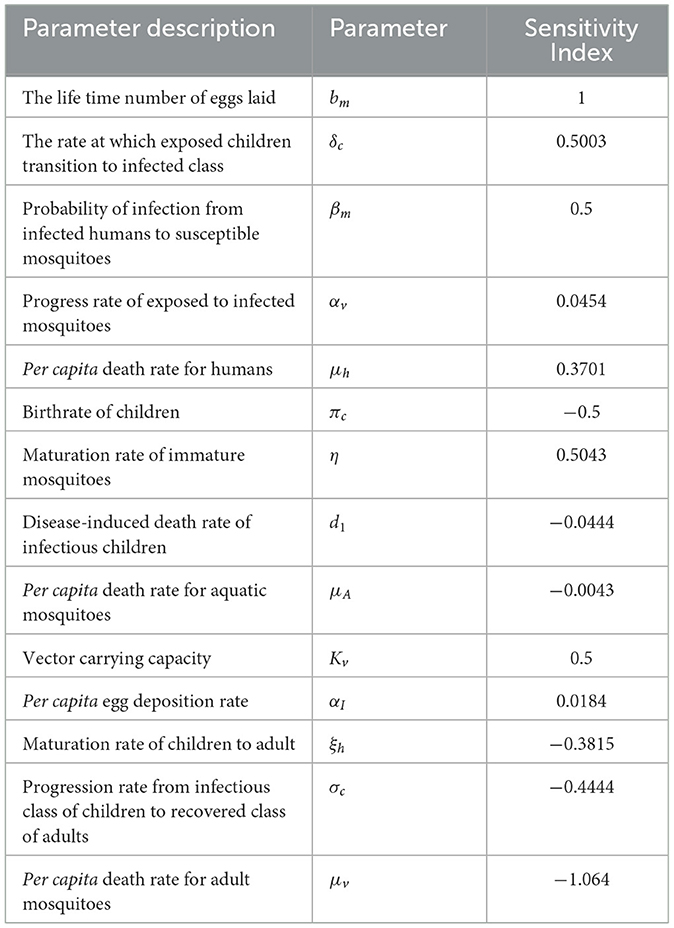
Table 4. Sensitivity analysis of the basic reproduction number (R0) at parameter values given above.
From the analysis of Table 4 and Figure 2, it is evident that each parameter has a positive or negative effect on the basic reproduction number (R0). Parameters with positive signs, such as bm, δc, βm, αv, μh, η, kv, and αI, increase R0, while those with negative signs, such as πc, d1, μA, ξh, σc, and μv, decrease it. The parameter with a higher sensitivity index magnitude is more influential than those with smaller magnitudes, as exhibited in Figure 2. For instance, among the parameters given in the fractional malaria model (14) relative to R0, the per capita death rate for adult mosquitoes (μv), the lifetime number of eggs laid (bm), the maturation rate of immature mosquitoes (η), vector carrying capacity(kv), and the rate at which exposed children transition to the infected class (δc) are the most sensitive parameters, in that order. Therefore, to eliminate or control malaria disease, it is important to focus on controlling these parameters.
6 Model analysis with climate-dependent (temperature and rainfall) parameter
This section examines the model parameters that affect malaria transmission dynamics focusing on temperature and rainfall. The results presented below were obtained using MATLAB software.
6.1 The mosquito maturation rate
The mosquito maturation rate, denoted by η(T,R), depends on both temperature (T) and rainfall (R). It determines the rate at which immature mosquitoes develop into mature adults, as described by the following equation [see [8, 14, 41] and the references therein].
where
• , where B(T) is the lifetime number of eggs laid,
• , where PE(R) is the daily survival probabilities of eggs,
• , where PL(R) is the daily survival probabilities of larva,
• , wherePP(R) is the daily survival probabilities of pupae,
• , where PL(T) is the temperature-dependent daily probability of survival of larvae,
• , where TEA(T) is the development time from egg to adult mosquito.
• Thus,
Based on the study of malaria transmission shown in [8, 14, 40, 41] and Figure 3, we examined the effects of temperature on the infected mosquito population in our proposed integer-order malaria model (14). We simulated infected mosquito populations across four temperature ranges: 17–25°C, 21–25°C, 30–32°C, and 35–39°C. The results are shown in Figures 4A–D, respectively.
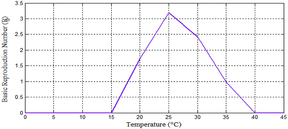
Figure 3. Relationship between basic reproduction number vs. temperature.
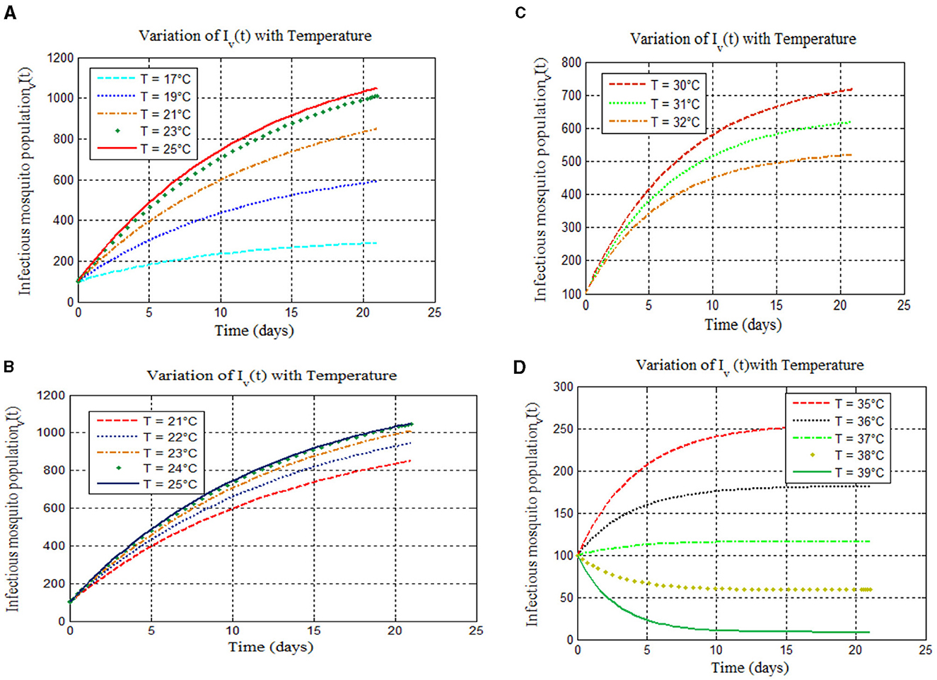
Figure 4. Model simulations 4 show new mosquito infections for temperatures: (A) (17–25°C), (B) (21–25°C), (C) (30–32°C), and (D) (35–39°C).
Furthermore, we investigated the effects of daily rainfall on mosquito development. Mosquito burden are known to peak at 25°C [[8, 40–42] and Figure 4A], so we used this constant temperature (T = 25°C) for our analysis, as in previous studies [see [42] and the reference therein]. Figure 5 depicts the relationship between mosquito maturation rate (η(T,R)) and rainfall (R) in millimeters for a temperature of 25°C. As shown in Figure 5, aquatic mosquitoes cannot survive daily rainfall exceeding 50 millimeters. It is important to note that aquatic mosquitoes cannot survive daily rainfall exceeding 50 mm, which limits vector population growth. These effects are illustrated in Figures 6A–D.
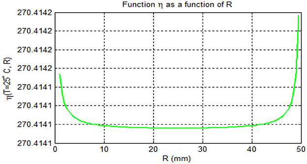
Figure 5. Mosquito maturation rate (η (T,R)) vs. rainfall (R) in mm for (T = 25).
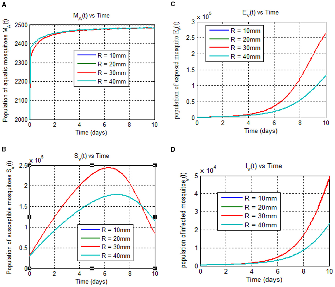
Figure 6. (A–D) Show mosquito stages (aquatic, susceptible, exposed, and infected) at 25°C over time (days) for different rainfall rates (10, 20, 30, and 40 mm).
The mosquito maturation rate, denoted by η(T,R), depends on both temperature (T) and rainfall (R). This rate determines the speed at which immature mosquitoes develop into mature adults. We examined this rate for various temperature and rainfall values: T = 20, 25, 30, and 35°C and R = 10, 20, 30, and 40 mm. The results are shown in Figure 6.
7 Results and discussion
7.1 Results
This section presents fractional-order (14) malaria models using graphs to understand the behavior of the solution trajectories. To draw the graph of the fractional-order model (13), we use the scheme introduced in [43], that is, from the solution of the differential equation with fractional order α given by
expressed as
where
At t = tn+1, n = 0, 1, 2, ⋯ , we obtain
With the help of interpolation polynomial, we approximate the function f(τ, g(τ))over [ti, ti+1].
Using Equation 110, Equation 109 takes the form:
Solving the integrals involved in Equation 111, we get the approximate solution as below:
Hence, we have the following recursive formulas for the proposed malaria model (14):
where
7.2 Discussion
Fractional-order malaria model analysis considering temperature and rainfall with Caputo operators showed correlation between these factors and mosquito population dynamics. Key factors affecting mosquito dynamics identified through sensitivity analysis were adult mosquito death rate, egg laying rate, maturation rate, vector carrying capacity, and exposed child transition rate, aligning with prior studies [8].
Based on the study of malaria transmission shown in [8, 14, 40–42] and Figure 3, we examined the effects of temperature on the infected mosquito population in our proposed integer-order malaria model 14(α = 1). We varied temperatures across four ranges: 17–25°C, 21–25°C, 30–32°C, and 35–39°C. The results are shown in Figures 4A–D, respectively. Figure 4A confirms that within the 17–25°C range, both infections and malaria burden rise with temperature, with the optimal temperature being 25°C [as expected from [8, 14, 40–42]]. However, Figures 4B–D show varying trends at higher temperatures: a peak burden at higher temperatures [Figure 4B, supported by [8]], a decrease with increasing temperature [Figure 4C, consistent with [8] and the references therein and [40]], and a drastic decrease with increasing temperature (Figure 4D) [see [15] and the references therein and [14, 40]].
As Figure 6A shows, the maximum value for aquatic mosquito vector growth is observed at a rainfall of 40 mm. In contrast, the remaining mosquito stages, including the susceptible mosquito (Figure 6B), exposed mosquito (Figure 6C), and infected mosquito (Figure 6D), all require a maximum rainfall of 30 mm for growth. Notably, infected mosquito populations peak at 30 mm of rainfall, suggesting that this is a favorable condition for malaria transmission compared to other rainfall values considered. Thus, we conclude that the peak for malaria transmission is at temperature (T = 25°C) [8, 40–42] and rainfall (R = 30 mm) [42]. Figure 7 reveals that mosquito maturation rate peaks and reaches its minimum at 20°C (19.18 and 10 mm, respectively) despite variations in rainfall (10–40 mm).
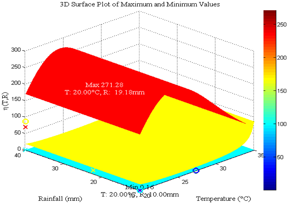
Figure 7. Impact of temperature and daily rainfall on mosquito maturation rate. Values used: T = 20, 25, 30, and 35°C and R = 10, 20, 30, and 40 mm.
Figure 8 shows mosquito infection peaks at 25°C for all fractional orders (α = 0.7, 0.8, 0.9, and 1), similar to the classical malaria model 14 (Figure 4A) and aligned with prior findings [8, 40–42]. In addition, Figures 8A–D (α = 0.7, 0.8, 0.9, and 1) reveal a rise in mosquito infections with increasing temperature, consistent with the classical model 14 (Figure 4A) [8], whereas Figures 9A–D for all fractional orders (α = 0.7, 0.8, 0.9, and 1) show a dramatic reduction in mosquito infection as the temperature increases from 35 to 39°C. This is similar to the graph of the classical malaria model (14) as in Figure 4D, which is consistent with the findings in [15] and the reference therein and [40].
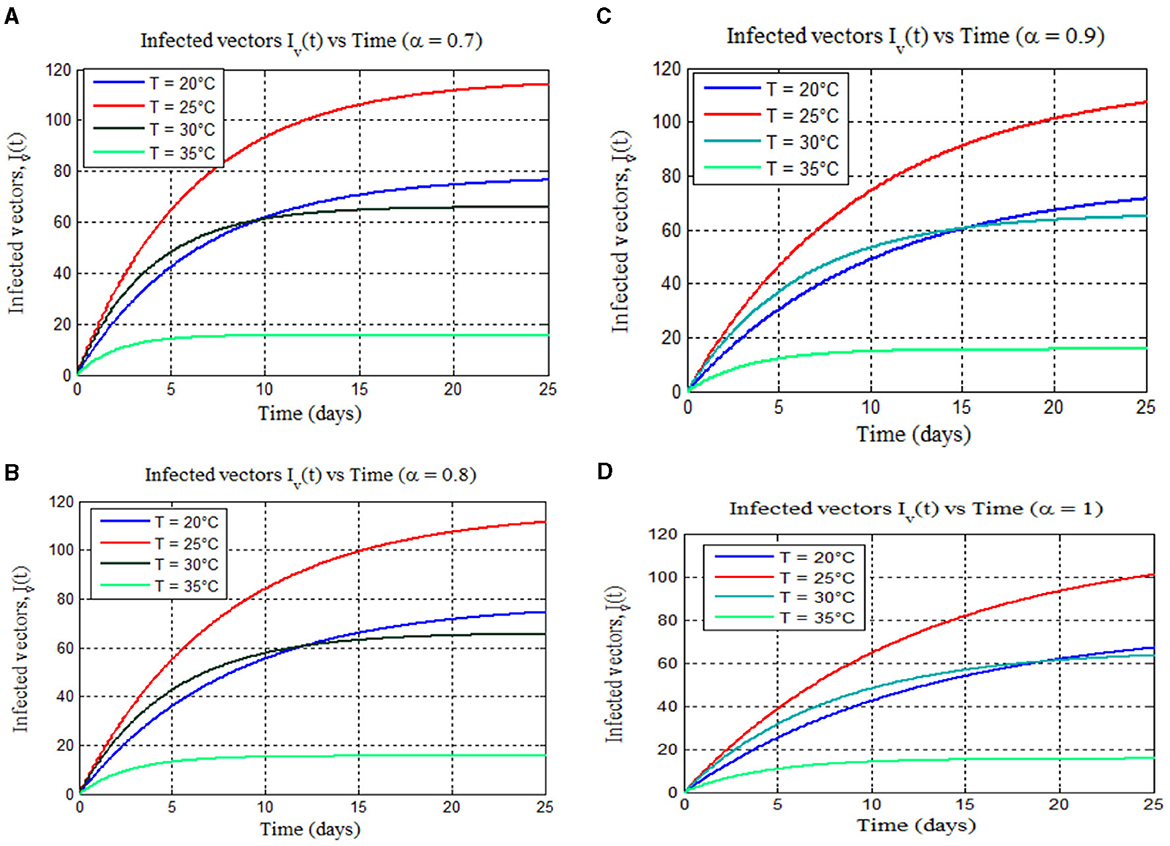
Figure 8. (A–D) Exemplify the total numbers of infected vectors for 17–25°C for different values of fractional order alpha: (A) (α = 0.7), (B) (α = 0.8), (C) (α = 0.9), and (D) (α = 1), respectively.
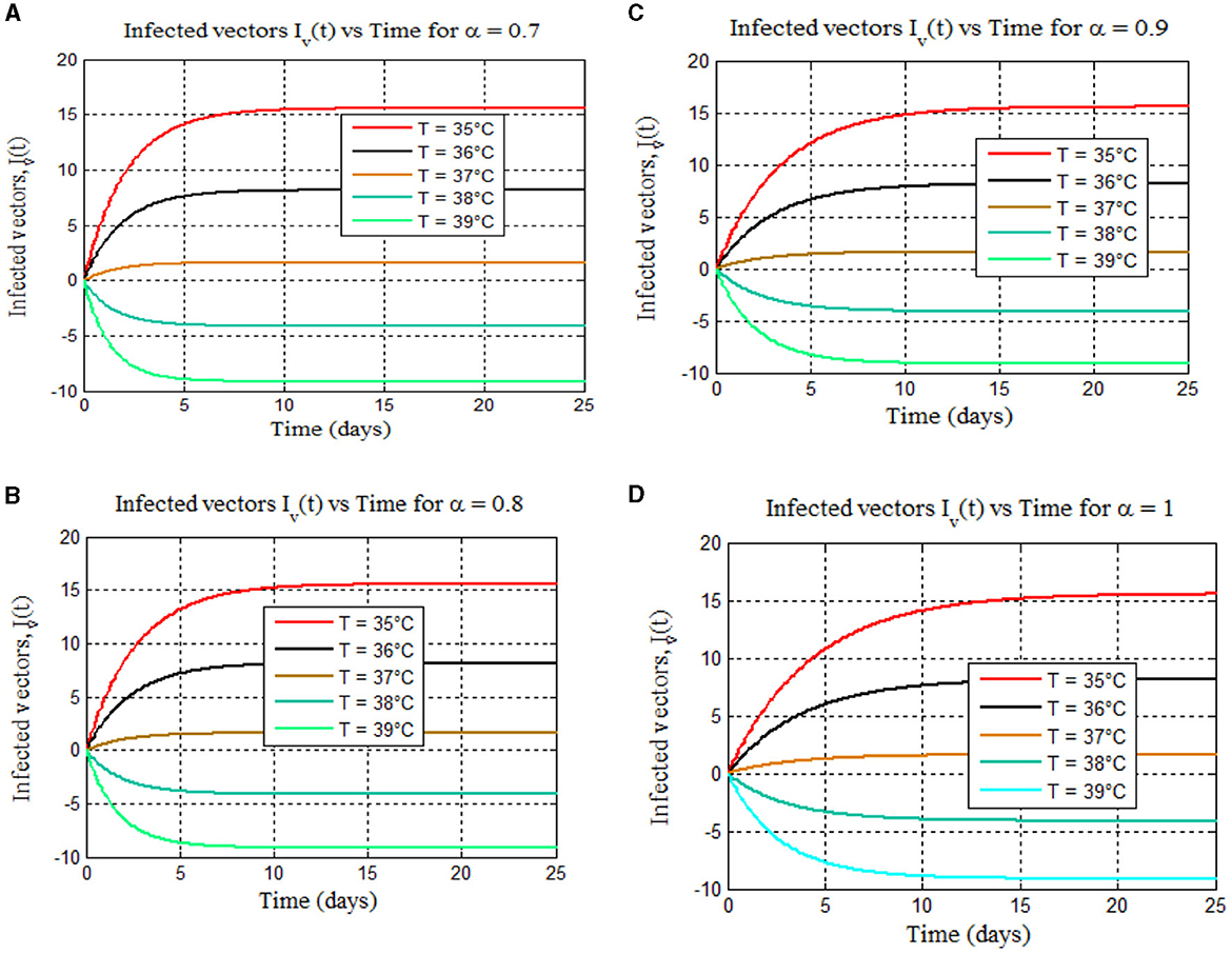
Figure 9. (A–D) Depict the total numbers of infected vectors for 35–39°C for different values of fractional order alpha: (A) (α = 0.7), (B) (α = 0.8), (C) (α = 0.9), and (D) (α = 1), respectively.
Furthermore, from Figures 8, 9, we can see that as the value of the fractional order alpha approaches 1, the results resemble the graph of the classical malaria model 14. For instance, Figures 8A–D (α = 0.7, 0.8, 0.9, and 1) resemble the classical malaria model 14 (α = 1) in Figure 4A, and Figures 9A–D (α = 0.7, 0.8, 0.9, and 1) resemble the classical malaria model 14 (α = 1) (Figure 4D).
Furthermore, Figure 10 shows that, like Figures 8A–D plotted on the different plane, the burden of mosquito peaks shown to occur at 25°C. As the value of the fractional-order derivative approaches one, it resembles Figure 4A, the classical model of 14 (α = 1). One advantage of ABC fractional derivative operators is that we can obtain distinct solutions.
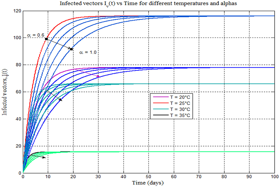
Figure 10. Infected vector vs. time (days) for different temperatures 17–25°C and different alphas (α = 0.6, 0.7, 0.8, 0.9, and 1).
Figure 11A demonstrates that as the number of susceptible children under seventeen decreases, the value of alpha (α) also decreases. This suggests a linear relationship between the two. Conversely, Figure 11B reveals that decreasing the exposed class of children under seventeen lowers alpha (α). This implies faster transitions from susceptible to exposed with a lower alpha value. Finally, Figure 11C shows a steeper curve. This indicates that model (14) relies heavily on past infection data when determining the rate of change in infected individuals.
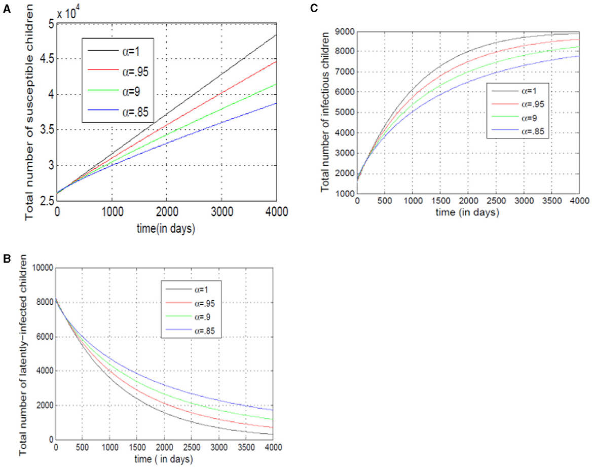
Figure 11. (A–C) Show the total numbers of susceptible, exposed, and infected children under 17, for different values of alpha.
Figures 12A–C examine adult susceptibility and disease spread. Figure 12A shows a rise and fall in susceptible adults, reflecting growth (new adults) followed by depletion (infections/immunity). Figure 12B reveals slower transitions from susceptible to exposed adults with lower alpha (α). Conversely, Figure 12C shows infected mosquitoes raise with higher alpha (α), implying the model prioritizes past infections in adult disease spread. The decline in infected adults with higher alpha (α) suggests the model incorporates other factors later.
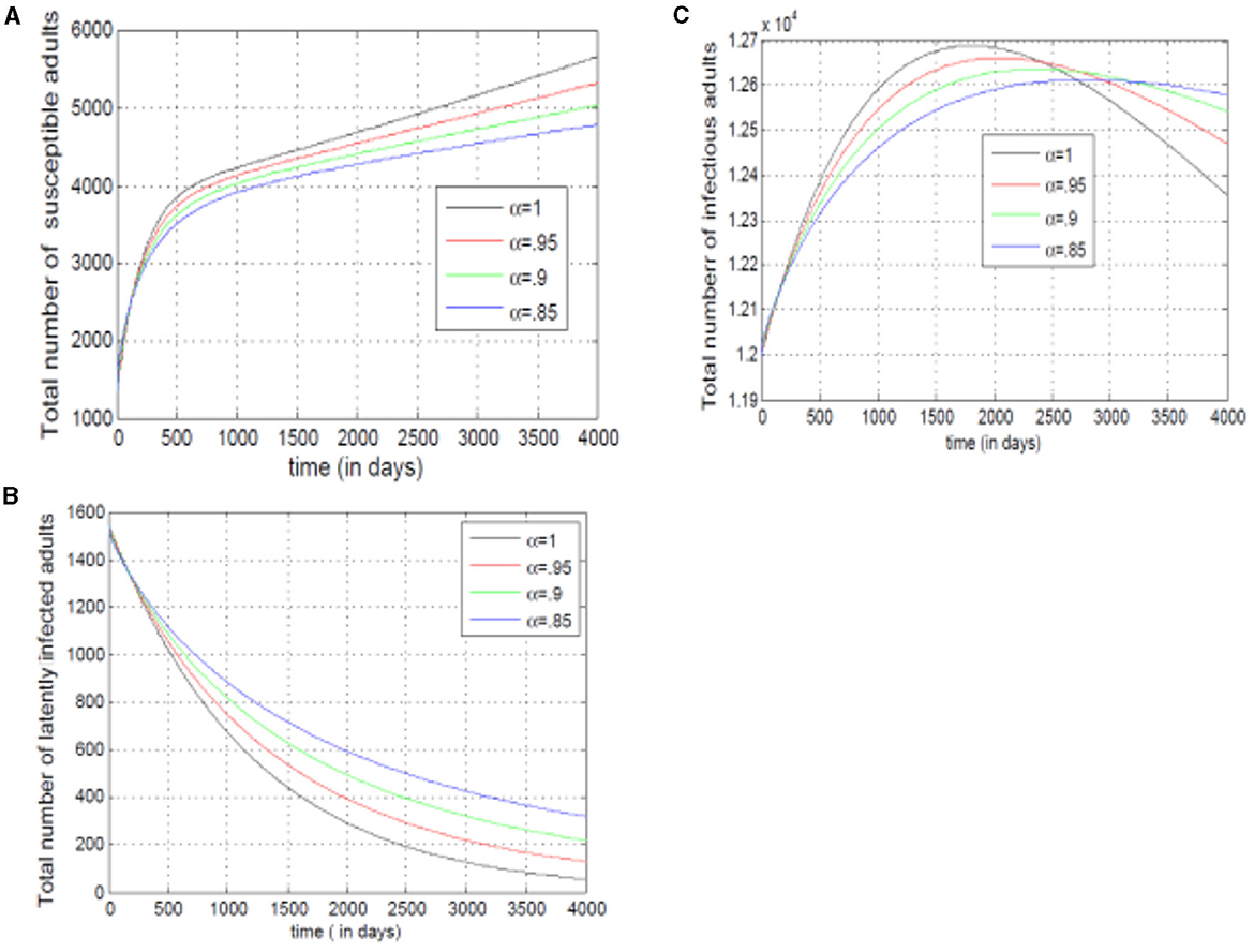
Figure 12. (A–C) Show the total numbers of susceptible, exposed, and infected adults, for different values of alpha.
Furthermore, for our future study, research directions [44–49] will be used. These areas, particularly those related to non-standard finite difference methods in fractional modeling [44, 49] and delay techniques in epidemic models [45–48], align well with the potential applications of our proposed method.
8 Conclusion
This study analyzes malaria transmission dependence on temperature and rainfall using a fractional-order differential model with Atangana–Baleanu operators (in the Caputo sense). It confirms the model's solution existence, uniqueness, and stability. Sensitivity analysis identified adult mosquito mortality, egg laying, maturation, and exposed child transition rates as key factors, aligning with prior research [8].
Simulations confirmed theoretical results: Peak malaria transmission occurred at 25°C (Figure 4A), consistent with [8, 40–42]. Malaria burden increased with temperature (17–25°C) (Figure 4A) [agreeing with [8]]. Figures 4B–D show a decrease with increasing temperature, also supported by [13–15], and the references therein.
Fractional-order model simulations (alpha approaching 1) resembled the classical model. For instance, Figures 8A–D (α = 0.7, 0.8, 0.9, and 1) resemble the classical malaria model in Figure 4A, and Figures 9A–D (α = 0.7, 0.8, 0.9, and 1) resemble Figure 4D. This study lays the groundwork for future research on infectious diseases using fractional derivatives, particularly ABC operators. Further extension could incorporate real-data non-autonomous parts, requiring additional compartments for mosquito and human populations.
Data availability statement
The original contributions presented in the study are included in the article/supplementary material, further inquiries can be directed to the corresponding author.
Ethics statement
Written informed consent was obtained from the individual(s), and minor(s)' legal guardian/next of kin, for the publication of any potentially identifiable images or data included in this article.
Author contributions
AG: Writing – original draft, Writing – review & editing, Conceptualization, Data curation, Formal analysis, Investigation, Methodology. CD: Writing – review & editing, Conceptualization, Formal analysis, Investigation, Software, Supervision.
Funding
The author(s) declare that no financial support was received for the research, authorship, and/or publication of this article.
Conflict of interest
The authors declare that the research was conducted in the absence of any commercial or financial relationships that could be construed as a potential conflict of interest.
Publisher's note
All claims expressed in this article are solely those of the authors and do not necessarily represent those of their affiliated organizations, or those of the publisher, the editors and the reviewers. Any product that may be evaluated in this article, or claim that may be made by its manufacturer, is not guaranteed or endorsed by the publisher.
References
1. Gbadamosi B, Adebimpe O, Ojo MM, Oludoun O, Abiodun O, Adesina I. Modeling the impact of optimal control measures on the dynamics of cholera. Model Earth Syst Environ. (2022) 9:1387–400. doi: 10.1007/s40808-022-01570-9
2. Malaria (2023). Available at: https://www.who.int/news-room/questions-and-answers/item/malaria (accessed November 30, 2023).
3. Xing Y, Guo Z, Liu J. Backward bifurcation in a malaria transmission model. J Biol Dyn. (2020) 14:368–88. doi: 10.1080/17513758.2020.1771443
4. Lakew YY, Fikrie A, Godana SB, Wariyo F, Seyoum W. Magnitude of malaria and associated factors among febrile adults in Siraro District Public Health facilities, West Arsi Zone, Oromia, Ethiopia 2022: a facility-based cross-sectional study. Malar J. (2023) 22:259. doi: 10.1186/s12936-023-04697-x
5. Ndamuzi E, Gahungu P. Mathematical modeling of malaria transmission dynamics: case of Burundi. J Appl Math Phys. (2021) 09:2447–60. doi: 10.4236/jamp.2021.910156
8. Okuneye K, Gumel AB. Analysis of a temperature- and rainfall-dependent model for malaria transmission dynamics. Math Biosci. (2017) 287:72–92. doi: 10.1016/j.mbs.2016.03.013
9. Traoré B, Sangaré B, Traoré S. A mathematical model of malaria transmission with structured vector population and seasonality. J Appl Math. (2017) 2017:1–15. doi: 10.1155/2017/6754097
10. Ducrot A, Sirima SB, Somé B, Zongo P. A mathematical model for malaria involving differential susceptibility, exposedness and infectivity of human host. J Biol Dyn. (2009) 3:574–98. doi: 10.1080/17513750902829393
11. Oheneba-Dornyo TV, Amuzu S, Maccagnan A, Taylor T. Estimating the impact of temperature and rainfall on malaria incidence in Ghana from 2012 to 2017. Environ Model Assess. (2022) 27:473–89. doi: 10.1007/s10666-022-09817-6
12. Parham PE, Michael E. Modeling the effects of weather and climate change on malaria transmission. Environ Health Perspect. (2010) 118:620–6. doi: 10.1289/ehp.0901256
13. Craig MH, Snow RW, le Sueur D. A climate-based distribution model of malaria transmission in sub-saharan Africa. Parasitol Today. (1999) 15:105–11. doi: 10.1016/s0169-4758(99)01396-4
14. Agusto FB, Gumel AB, Parham PE. Qualitative assessment of the role of temperature variations on malaria transmission dynamics. J Biol Syst. (2015) 23:1550030. doi: 10.1142/s0218339015500308
15. Agusto FB. Optimal control and temperature variations of malaria transmission dynamics. Complexity. (2020) 2020:1–32. doi: 10.1155/2020/5056432
16. Shah K, Sinan M, Abdeljawad T, El-Shorbagy MA, Abdalla B, Abualrub MS, et al. Detailed study of a fractal-fractional transmission dynamical model of viral infectious disease with vaccination. Complexity. (2022) 2022:1–21. doi: 10.1155/2022/7236824
17. Sidi Ammi MR, Tahiri M, Tilioua M, Zeb A, Khan I, Andualem M. Global analysis of a time fractional order spatio-temporal SIR model. Sci Rep. (2022) 12:5751. doi: 10.1038/s41598-022-08992-6
18. Mandal M, Jana S, Nandi SK, Kar TK. Modelling and control of a fractional-order epidemic model with fear effect. Energy Ecol Environ. (2020) 5:421–32. doi: 10.1007/s40974-020-00192-0
19. Windarto, Khan MA, Fatmawati. Parameter estimation and fractional derivatives of dengue transmission model. AIMS Math. (2020) 5:2758–79. doi: 10.3934/math.2020178
20. Tuan NH, Mohammadi H, Rezapour S. A mathematical model for COVID-19 transmission by using the Caputo fractional derivative. Chaos Solit Fract. (2020) 140:110107. doi: 10.1016/j.chaos.2020.110107
21. Atangana A, Baleanu D. New fractional derivatives with nonlocal and non-singular kernel: theory and application to heat transfer model. Therm Sci. (2016) 20:763–9. doi: 10.2298/tsci160111018a
22. Caputo M, Fabrizio M. A new definition of fractional derivative without singular kernel. Prog Fract Differ Appl. (2015) 9:15–23.
23. Caputo M. Linear models of dissipation whose Q is almost frequency independent–II. Geophys J Int. (1967) 13:529–39. doi: 10.1111/j.1365-246x.1967.tb02303.x
24. Gizaw AK, Deressa CT. Analysis of age-structured mathematical model of malaria transmission dynamics via classical and ABC fractional operators. Math Probl Eng. (2024) 2024:1–24. doi: 10.1155/2024/3855146
25. Ullah S, Altaf Khan M, Farooq MO, Alzahrani E. A fractional model for the dynamics of tuberculosis (TB) using Atangana-Baleanu derivative. Discrete Cont Dyn Syst. (2020) 13:937–56. doi: 10.3934/dcdss.2020055
26. Yavuz M. European option pricing models described by fractional operators with classical and generalized Mittag-Leffler kernels. Numer Methods Partial Differ Equ. (2021) 37:342–62. doi: 10.1002/num.22645
27. Deressa CT, Duressa GF. Analysis of Atangana–Baleanu fractional-order SEAIR epidemic model with optimal control. Adv Differ Equ. (2021) 2021:174. doi: 10.1186/s13662-021-03334-8
28. Deressa CT, Etemad S, Rezapour S. On a new four-dimensional model of memristor-based chaotic circuit in the context of nonsingular Atangana–Baleanu–Caputo operators. Adv Differ Eq. (2021) 2021:444. doi: 10.1186/s13662-021-03600-9
29. Yadeta DM, Gizaw AK, Mussa YO. Approximate analytical solution of one-dimensional beam equations by using time-fractional reduced differential transform method. J Appl Math. (2020) 2020:1–13. doi: 10.1155/2020/7627385
30. Odibat ZM, Shawagfeh NT. Generalized Taylor's formula. Appl Math Comput. (2007) 186:286–93. doi: 10.1016/j.amc.2006.07.102
31. Adel W, Elsonbaty A, Aldurayhim A, El-Mesady A. Investigating the dynamics of a novel fractional-order monkeypox epidemic model with optimal control. Alexand Eng J. (2023) 73:519–42. doi: 10.1016/j.aej.2023.04.051
32. Diekmann O, Heesterbeek JAP, Metz JAJ. On the definition and the computation of the basic reproduction ratio R 0 in models for infectious diseases in heterogeneous populations. J Math Biol. (1990) 28:365–82. doi: 10.1007/bf00178324
33. Van den Driessche P, Watmough J. Reproduction numbers and sub-threshold endemic equilibria for compartmental models of disease transmission. Math Biosci. (2002) 180:29–48. doi: 10.1016/s0025-5564(02)00108-6
34. Ahmed E, El-Sayed AMA, El-Saka HAA. On some Routh–Hurwitz conditions for fractional order differential equations and their applications in Lorenz, Rössler, Chua and Chen systems. Phys Lett A. (2006) 358:1–4. doi: 10.1016/j.physleta.2006.04.087
35. Vargas-De-León C. Volterra-type Lyapunov functions for fractional-order epidemic systems. Commun Nonlinear Sci Numer Simul. (2015) 24:75–85. doi: 10.1016/j.cnsns.2014.12.013
36. Bebernes JW. The stability of dynamical systems (J. P Lasalle). SIAM Rev. (1979) 21:418–20. doi: 10.1137/1021079
37. Sahnoune MY, Ez-Zetouni A, Akdim K, Zahid M. Qualitative analysis of a fractional-order two-strain epidemic model with vaccination and general non-monotonic incidence rate. Int J Dyn Control. (2023) 11:1532–43. doi: 10.1007/s40435-022-01083-4
38. Huo J, Zhao H, Zhu L. The effect of vaccines on backward bifurcation in a fractional order HIV model. Nonlinear Anal. (2015) 26:289–305. doi: 10.1016/j.nonrwa.2015.05.014
39. Chitnis N, Hyman JM, Cushing JM. Determining important parameters in the spread of malaria through the sensitivity analysis of a mathematical model. Bull Math Biol. (2008) 70:1272. doi: 10.1007/s11538-008-9299-0
40. Mordecai EA, Paaijmans KP, Johnson LR, Balzer C, Ben-Horin T, de Moor E, et al. Optimal temperature for malaria transmission is dramatically lower than previously predicted. Ecol Lett. (2013) 16:22–30. doi: 10.1111/ele.12015
41. Abdulaziz YA, Mukhtar JB, Rachid Ouifki M. Assessing the role of climate factors on malaria transmission dynamics in South Sudan. Math Biosci. (2019) 310:13–23. doi: 10.1016/j.mbs.2019.01.002
42. Yiga V, Nampala H, Tumwiine J. Analysis of the model on the effect of seasonal factors on malaria transmission dynamics. J Appl Math. (2020) 2020:1–19. doi: 10.1155/2020/8885558
43. Toufik M, Atangana A. New numerical approximation of fractional derivative with non-local and non-singular kernel: Application to chaotic models. Eur Phys J Plus. (2017) 132:444. doi: 10.1140/epjp/i2017-11717-0
44. Raza A, Rocha E, Fadhal E, Ibrahim RIH, Afkar E, Bilal M. The effect of delay techniques on a lassa fever epidemic model. Complexity. (2024) 2024:2075354. doi: 10.1155/2024/2075354
45. Raza A, Abdella K. Analysis of the dynamics of anthrax epidemic model with delay. Deleted J. (2024) 6:128. doi: 10.1007/s42452-024-05763-y
46. Alfwzan WF, Raza A, Martin-Vaquero J, Baleanu D, Rafiq M, Ahmed N, et al. Modeling and transmission dynamics of Zika virus through efficient numerical method. AIP Adv. (2023) 13:8945. doi: 10.1063/5.0168945
47. Raza A. Mathematical modelling of rotavirus disease through efficient methods. Comp Mater Cont. (2022) 72:4727–40. doi: 10.32604/cmc.2022.027044
48. Deresse AT, Mussa YO, Gizaw AK. Approximate analytical solution of two-dimensional nonlinear time-fractional damped wave equation in the caputo fractional derivative operator. Math Probl Eng. (2022) 2022:1–28. doi: 10.1155/2022/7004412
49. Gizaw AK, Mussa YO. Approximate analytical solutions of two-dimensional time fractional Kleingordon Equation. Ethiop J Educ Sci. (2022) 16:1–16. Retrieved from: https://ejhs.ju.edu.et/index.php/ejes/article/view/3956
Keywords: basic reproduction number, Mittag-Leffler function, stability analysis, sensitivity analysis, numerical simulations, global stability
Citation: Gizaw AK and Deressa CT (2024) Fractional-order analysis of temperature- and rainfall-dependent mathematical model for malaria transmission dynamics. Front. Appl. Math. Stat. 10:1396650. doi: 10.3389/fams.2024.1396650
Received: 06 March 2024; Accepted: 06 September 2024;
Published: 09 October 2024.
Edited by:
Fahad Al Basir, Asansol Girls' College, IndiaReviewed by:
Dipo Aldila, University of Indonesia, IndonesiaAli Raza, The University of Chenab, Pakistan
Copyright © 2024 Gizaw and Deressa. This is an open-access article distributed under the terms of the Creative Commons Attribution License (CC BY). The use, distribution or reproduction in other forums is permitted, provided the original author(s) and the copyright owner(s) are credited and that the original publication in this journal is cited, in accordance with accepted academic practice. No use, distribution or reproduction is permitted which does not comply with these terms.
*Correspondence: Ademe Kebede Gizaw, a2ViZWRlYWRlbWUyMDIwQGdtYWlsLmNvbQ==
†ORCID: Ademe Kebede Gizaw orcid.org/0000-0003-1061-6346
Chernet Tuge Deressa orcid.org/0000-0002-7990-9430