Beta transformation of the Exponential-Gaussian distribution with its properties and applications

This study introduces a five-parameter continuous probability model named the Beta-Exponential-Gaussian distribution by extending the three-parameter Exponential-Gaussian distribution with the beta transformation method. The basic properties of the new distribution, including reliability measure, hazard function, survival function, moment, skewness, kurtosis, order statistics, and asymptotic behavior, are established. Using the acceptance-rejection algorithm, simulation studies are conducted. The new model is fitted to the simulated and real data sets, and its performance is reported. The Beta-Exponential-Gaussian distribution is found to be more flexible and has better performance in many aspects. It is suggested that the new distribution would be used in modeling data having skewness and bimodal distribution.

1 Introduction

The beta distribution family gained popularity a few years ago, and various studies have been conducted on beta compounding with other distributions such as Beta-Frechet [1], Beta-Gumbel [2], Beta-Pareto [3], Beta-Gamma [4], Beta-Gompertz [5], Beta-Normal[6], Beta-Power [7], Beta-Weibull [8], Beta-Exponentiated Weibull [9], Beta-Modified Weibull [10], Beta-Extended Weibull[11], the Beta-Generalized Logistic [12], Beta-Log-Logistic [13], Beta-Exponential [14], Beta-Generalized Exponential [15], Beta-Moyal [16], Beta-Generalized Half-Normal [17], Beta-Dagum [18], Beta-Laplace [19], Beta-Burr XII [20], Beta-Generalized Pareto [21], Beta-Cauchy [22], Beta-Half-Cauchy [23], Beta-Exponentiated Pareto [24], Beta-Log-Logistic [13], Beta-Type I Generalized Half Logistic [25], Beta-Bessel Distributions [26], Beta-Rayleigh Distribution [27], Beta-Exponentiated Lindley [28], Beta-Lindley [29], Beta-Lindley-Poisson Distribution [30], and Beta-Lindley Geometric Distribution [31].

This study presents a five-parameter distribution called the Beta-Exponential-Gaussian distribution, which extends the Ex-Gaussian distribution by adding two additional parameters to control its skewness and kurtosis.

In cognitive psychology research, the Ex-Gaussian distribution is used to examine the semantic stroop effect [32], reading eye movements [33], and response time distributions [34]. Additionally, it is utilized to mimic fixation lengths [35], which are frequently employed in eye-tracking research as a gauge of cognitive processes.

This investigation unfolds to examine the new Beta-Ex-Gaussian distribution. In Section 2, a parent sub-model, the basic Ex-Gaussian distribution is introduced. The transformation technique for the proposed distribution is explained in Section 3. Methodically, Section 4 examines the Beta-Ex-Gaussian distribution. Advancing to Section 5, visual representations of the probability density function (PDF) and cumulative distribution function (CDF) of the Beta-Ex-Gaussian distribution are presented. Section 6 investigates statistical distinctions by deriving expressions for moments. The discourse within Section 7 explores the sphere of order statistics. Survival and hazard functions are scrutinized in Section 8. In Section 9, attention is directed toward estimation methodologies, with an emphasis on maximum likelihood. Section 10 offers simulation results from a comprehensive acceptance-rejection process. Section 11 expounds on four practical applications. Finally, Section 12 provides a conclusive conclusion, thereby concluding the article.

2 Basic exponential-Gaussian distribution

The exponential-Gaussian (Ex-Gaussian), also called the exponentially modified Gaussian (EMG) distribution, is a probability distribution that convolutions exponential and normal random variables and is used in signal processing, finance, and neuroscience for skewness and heavy tails data. It has a closed-form probability density function and a cumulative distribution function, making it useful for statistical analysis [36–39]. For ∀μ ∈ ℝ, σ, λ > 0, and ∀x ∈ ℝ, its PDF, CDF, Hazard, and Survival functions are given in the Equations (1–4), respectively.

$\begin{array}{ll}f\left(x;\mu ,\lambda ,\sigma \right)=\frac{\lambda }{2}exp\left(\frac{\lambda }{2}\left(2\mu +\lambda {\sigma }^2-2x\right)\right)\text{erfc}\left(\frac{\mu +\lambda {\sigma }^2-x}{\sigma \sqrt{2}}\right)& (1)\end{array}$

$\begin{array}{l}F\left(x;\mu ,\lambda ,\sigma \right)\\ =\frac{1}{2}\text{erfc}\left(\frac{\mu -x}{\sigma \sqrt{2}}\right)-\frac{1}{2}exp\left(\frac{\lambda }{2}\left(2\mu +\lambda {\sigma }^2-2x\right)\right)\\ \hspace{1em}\hspace{1em}\hspace{1em}\hspace{1em}\hspace{1em}erfc\left(\frac{\mu +\lambda {\sigma }^2-x}{\sigma \sqrt{2}}\right)& (2)\end{array}$

$\begin{array}{l}\hspace{1em}\hspace{1em}\hspace{1em}\hspace{1em}\hspace{1em}\hspace{1em}\hspace{1em}h\left(x\right)=\frac{f\left(x\right)}{1-F\left(x\right)}\\ =\frac{\frac{\lambda }{2}exp\left(\frac{\lambda }{2}\left(2\mu +\lambda {\sigma }^2-2x\right)\right)\text{erfc}\left(\frac{\mu +\lambda {\sigma }^2-x}{\sigma \sqrt{2}}\right)}{1-\frac{1}{2}\text{erfc}\left(\frac{\mu -x}{\sigma \sqrt{2}}\right)+\frac{1}{2}exp\left(\frac{\lambda }{2}\left(2\mu +\lambda {\sigma }^2-2x\right)\right)erfc\left(\frac{\mu +\lambda {\sigma }^2-x}{\sigma \sqrt{2}}\right)}& (3)\end{array}$

$\begin{array}{l}S\left(x\right)=1-F\left(x\right)=1-\frac{1}{2}\text{erfc}\left(\frac{\mu -x}{\sigma \sqrt{2}}\right)\\ +\frac{1}{2}exp\left(\frac{\lambda }{2}\left(2\mu +\lambda {\sigma }^2-2x\right)\right)erfc\left(\frac{\mu +\lambda {\sigma }^2-x}{\sigma \sqrt{2}}\right)& (4)\end{array}$

where erfc is the complementary error function defined by $erfc\left(x\right)=\frac{2}{\sqrt{\pi }}{\int }_x^{\infty }{e}^{-t^2}dt$.

3 Transformation techniques

Many transformation methods were applied to generate new probability distributions. This study uses the beta-generated (B-G) approach to generate continuous probability distributions. This technique modifies a base distribution using a generator function, resulting in a variety of shapes and characteristics. The beta distribution is used as the generator, adding more parameters to fit different shapes and determining skewness by the sum of all forms [40].

Let f(x; Θ) and F(x; Θ) be the probability density function and the cumulative distribution function (cdf) of a random variable X, respectively, where Θ is a p × 1 parameter vector, and then the cumulative distribution function is generated by applying [6, 29]

$\begin{array}{l}G\left(x;\alpha ,\beta ,\Theta \right)=\frac{1}{B\left(\alpha ,\beta \right)}{\displaystyle \underset{0}{\overset{F\left(x;\Theta \right)}{\int }}}{t}^{\alpha -1}{\left(1-t\right)}^{\beta -1}dt=\frac{B\left(F\left(x;\Theta \right);\alpha ,\beta \right)}{B\left(\alpha ,\beta \right)}\\ \hspace{1em}\hspace{1em}\hspace{1em}\hspace{1em}=I_{F\left(x;\Theta \right)}\left(\alpha ,\beta \right),-\infty <x<\infty ,& (5)\end{array}$

where α > 0 and β > 0 are two additional parameters whose role is to introduce skewness and vary the tail weight. $B\left(\alpha ,\beta \right)={\int }_0^1{t}^{\alpha -1}{\left(1-t\right)}^{\beta -1}dt=\frac{\Gamma \left(\alpha \right)\Gamma \left(\beta \right)}{\Gamma \left(\alpha +\beta \right)}$ is the beta function, $B\left(y;\alpha ,\beta \right)={\int }_0^y{t}^{\alpha -1}{\left(1-t\right)}^{\beta -1}dt$ is the incomplete beta function with B(α, β) = B₁(α, β), and $I_y\left(\alpha ,\beta \right)=\frac{B\left(y;\alpha ,\beta \right)}{B\left(\alpha ,\beta \right)}$ is the incomplete beta function ratio. The corresponding probability density function of Equation (5) is then given as follows:

$\begin{array}{ll}g\left(x\right)=\frac{1}{B\left(\alpha ,\beta \right)}F{\left(x\right)}^{\alpha -1}{\left(1-F\left(x\right)\right)}^{\beta -1}f\left(x\right),-\infty <x<\infty ,& (6)\end{array}$

This family of distributions can be considered as generalization of the distribution of order statistics [40] for the random variable X with CDF F(x). When α and β are integers, Equation (6) is the α^th order statistic of the random sample of size (α+β−1).

4 The new Beta-Ex-Gaussian(BExG) distribution

Let F(x; Θ) be the baseline CDF of an Ex-Gaussian, a continuous random variable, with Θ = (μ, σ, λ) as parameter vectors. We now introduce the five-parameter Beta-Ex-Gaussian (BExG) distribution by taking G(x) from Equation (5), the CDF of Equation (6). Substituting F(x; Θ) in Equation (5) by the CDF Equation (2) yields the CDF of the BExG as follows:

$\begin{array}{l}G(x)=\frac{1}{B(\alpha ,\beta )}{\displaystyle \underset{0}{\overset{F(x;\Theta )}{\int }}{t}^{\alpha -1}}{(1-t)}^{\beta -1}dt=I_{F(x;\Theta )}(\alpha ,\beta )\\ =\frac{1}{B(\alpha ,\beta )}{\int }_0^{\frac{1}{2}\text{erfc}\left(\frac{\mu -x}{\sigma \sqrt{2}}\right)-\frac{1}{2}\exp \left(\frac{\lambda }{2}(2\mu +\lambda {\sigma }^2-2x)\right)\mathrm{erfc}\left(\frac{\mu +\lambda {\sigma }^2-x}{\sigma \sqrt{2}}\right)}\\ t^{\alpha -1}{(1-t)}^{\beta -1}dt\\ =I_{\frac{1}{2}\text{erfc}\left(\frac{\mu -x}{\sigma \sqrt{2}}\right)-\frac{1}{2}\exp \left(\frac{\lambda }{2}(2\mu +\lambda {\sigma }^2-2x)\right)\mathrm{erfc}\left(\frac{\mu +\lambda {\sigma }^2-x}{\sigma \sqrt{2}}\right)}\left(\alpha ,\beta \right)\\ G(x)=\frac{1}{B(\alpha ,\beta )}B(\frac{1}{2}\text{erfc}\left(\frac{\mu -x}{\sigma \sqrt{2}}\right)-\frac{1}{2}\exp \left(\frac{\lambda }{2}(2\mu +\lambda {\sigma }^2-2x)\right)\\ \mathrm{erfc}\left(\frac{\mu +\lambda {\sigma }^2-x}{\sigma \sqrt{2}}\right);\alpha ,\beta )& (7)\end{array}$

where α > 0 and β > 0 are new parameters that controls the skewness and kurtosis of the distribution, i.e., the distribution's shape, and ∀μ ∈ ℝ, σ, λ > 0, and ∀x ∈ ℝ are the location, scale, and rate parameters, respectively. A random variable X with the CDF Equation (7) is said to have a BExG distribution and will be denoted by X~BExG(Φ), where Φ = (μ, σ, λ, α, β).

For any values of α and β, we can write Equation (5) in terms of the well-known hypergeometric function (see [1, 5, 7]) given as follows:

$\begin{array}{ll}G\left(x\right)=\frac{F{\left(x\right)}^{\alpha }}{\alpha B\left(\alpha ,\beta \right)}{}_2{F}_1\left(\alpha ,1-\beta ,\alpha +1;F\left(x\right)\right)& (8)\end{array}$

Theorem 1. The new random variable X for x ∈ ℝ, λ > 0, μ ∈ ℝ, σ > 0, α > 0, and β > 0 having cumulative distribution function (CDF) and probability density function (PDF) expressed as follows:

1. Cumulative distribution function (CDF):

$\begin{array}{l}\mathrm{Gs}(x)=\\ \frac{{\left(\frac{1}{2}\mathrm{erfc}\left(\frac{\mu -x}{\sigma \sqrt{2}}\right)-\frac{1}{2}\exp \left(\frac{\lambda }{2}(2\mu +\lambda {\sigma }^2-2x)\right)\mathrm{erfc}\left(\frac{\mu +\lambda {\sigma }^2-x}{\sigma \sqrt{2}}\right)\right)}^{\alpha }}{\alpha B(\alpha ,\beta )}\times \\ {}_{2}F{}_1(\alpha ,1-\beta ,\alpha +1;\frac{1}{2}\mathrm{erfc}\left(\frac{\mu -x}{\sigma \sqrt{2}}\right)\\ -\frac{1}{2}\exp \left(\frac{\lambda }{2}(2\mu +\lambda {\sigma }^2-2x)\right)\mathrm{erfc}\left(\frac{\mu +\lambda {\sigma }^2-x}{\sigma \sqrt{2}}\right))& (9)\end{array}$

2. Probability density function (PDF):

$\begin{array}{l}g\left(x\right)=\frac{1}{B\left(\alpha ,\beta \right)}(\frac{1}{2}erfc\left(\frac{\mu -x}{\sigma \sqrt{2}}\right)-\frac{1}{2}exp\left(\frac{\lambda }{2}\left(2\mu +\lambda {\sigma }^2-2x\right)\right)\\ erfc\left(\frac{\mu +\lambda {\sigma }^2-x}{\sigma \sqrt{2}}\right){)}^{\alpha -1}\\ \times (1-\frac{1}{2}[erfc\left(\frac{\mu -x}{\sigma \sqrt{2}}\right)-exp\left(\frac{\lambda }{2}\left(2\mu +\lambda {\sigma }^2-2x\right)\right)\\ erfc\left(\frac{\mu +\lambda {\sigma }^2-x}{\sigma \sqrt{2}}\right)]{)}^{\beta -1}\\ \times (\frac{\lambda }{2}exp\left(\frac{\lambda }{2}\left(2\mu +\lambda {\sigma }^2-2x\right)\right)erfc\left(\frac{\mu +\lambda {\sigma }^2-x}{\sigma \sqrt{2}}\right))& (10)\end{array}$

g(x)≥0

${\int }_0^{\infty }g\left(x\right)dx=1$

where ${}_2{F}_1\left(a,b,c,z\right)={\sum }_{k=0}^{\infty }\frac{\left({\left(a\right)}_k{\left(b\right)}_k\right)}{\left({\left(c\right)}_{k}k!\right)}{z}^k$ and (a)_k = a(a+1)⋯(a+k−1).

Proof.

1. Using Equation (8), we can prove for G(x) in Equation (9) and substituting the given expression for F(x) in Equation (2) into Equation (8), we get:

$\begin{array}{l}G(x)=\\ \frac{{\left(\frac{1}{2}\mathrm{erfc}\left(\frac{\mu -x}{\sigma \sqrt{2}}\right)-\frac{1}{2}\exp \left(\frac{\lambda }{2}(2\mu +\lambda {\sigma }^2-2x)\right)\mathrm{erfc}\left(\frac{\mu +\lambda {\sigma }^2-x}{\sigma \sqrt{2}}\right)\right)}^{\alpha }}{\alpha B(\alpha ,\beta )}\\ \times {}_{2}F{}_1(\alpha ,1-\beta ,\alpha +1;\frac{1}{2}\mathrm{erfc}\left(\frac{\mu -x}{\sigma \sqrt{2}}\right)\\ -\frac{1}{2}\exp \left(\frac{\lambda }{2}(2\mu +\lambda {\sigma }^2-2x)\right)\mathrm{erfc}\left(\frac{\mu +\lambda {\sigma }^2-x}{\sigma \sqrt{2}}\right))\end{array}$

2. The proof of the probability density function in Equation (10) involves a substitution method. This is achieved by substituting the expressions for F(x) and f(x) from Equations (1, 2) into Equation (6). The resulting expression for g(x) is provided as follows:

$\begin{array}{l}g\left(x\right)=\frac{1}{B\left(\alpha ,\beta \right)}(\frac{1}{2}erfc\left(\frac{\mu -x}{\sigma \sqrt{2}}\right)\\ -\frac{1}{2}exp\left(\frac{\lambda }{2}\left(2\mu +\lambda {\sigma }^2-2x\right)\right)erfc\left(\frac{\mu +\lambda {\sigma }^2-x}{\sigma \sqrt{2}}\right){)}^{\alpha -1}\\ \times (1-\frac{1}{2}[erfc\left(\frac{\mu -x}{\sigma \sqrt{2}}\right)-exp\left(\frac{\lambda }{2}\left(2\mu +\lambda {\sigma }^2-2x\right)\right)\\ erfc\left(\frac{\mu +\lambda {\sigma }^2-x}{\sigma \sqrt{2}}\right)]{)}^{\beta -1}\\ \times (\frac{\lambda }{2}exp\left(\frac{\lambda }{2}\left(2\mu +\lambda {\sigma }^2-2x\right)\right)erfc\left(\frac{\mu +\lambda {\sigma }^2-x}{\sigma \sqrt{2}}\right))\end{array}$

This function, g(x) in (2a), is always non-negative, which is trivial to prove, and

$\begin{array}{l}{\displaystyle {\int }_{-\infty }^{\infty }}g\left(x\right)dx=1={\displaystyle {\int }_{-\infty }^0}g\left(x\right)dx+{\displaystyle {\int }_0^{\infty }}g\left(x\right)dx\\ =0+{\displaystyle {\int }_0^{\infty }}g\left(x\right)dx=1\forall x\in \text{R}\end{array}$

To prove (2b) integrates is 1 over the real number, we used Equation (6) for g(x)

${\displaystyle {\int }_0^{\infty }}g\left(x\right)dx={\displaystyle {\int }_0^{\infty }}\frac{1}{B\left(\alpha ,\beta \right)}F{\left(x\right)}^{\alpha -1}{\left(1-F\left(x\right)\right)}^{\beta -1}f\left(x\right)dx$

Use integration by substitution: u = F(x) and differentiate u with respect to x, yielding:

$\begin{array}{l}{\displaystyle {\int }_0^{\infty }}g\left(x\right)dx={\displaystyle {\int }_0^{\infty }}\frac{1}{B\left(\alpha ,\beta \right)}{u}^{\alpha -1}{\left(1-u\right)}^{\beta -1}du\\ \hspace{1em}\hspace{1em}=\frac{1}{B\left(\alpha ,\beta \right)}{\displaystyle {\int }_0^{\infty }}{u}^{\alpha -1}{\left(1-u\right)}^{\beta -1}du\end{array}$

The integral ${\int }_0^{\infty }{u}^{\alpha -1}{\left(1-u\right)}^{\beta -1}du$ is a special case of the beta function, defined as:

$B\left(\alpha ,\beta \right)={\displaystyle {\int }_0^1}{u}^{\alpha -1}{\left(1-u\right)}^{\beta -1}du$

Table 1 shows that some closed-form expansions for Equation (5) distribution based on real, non-integer, or integer parameters.

Table 1

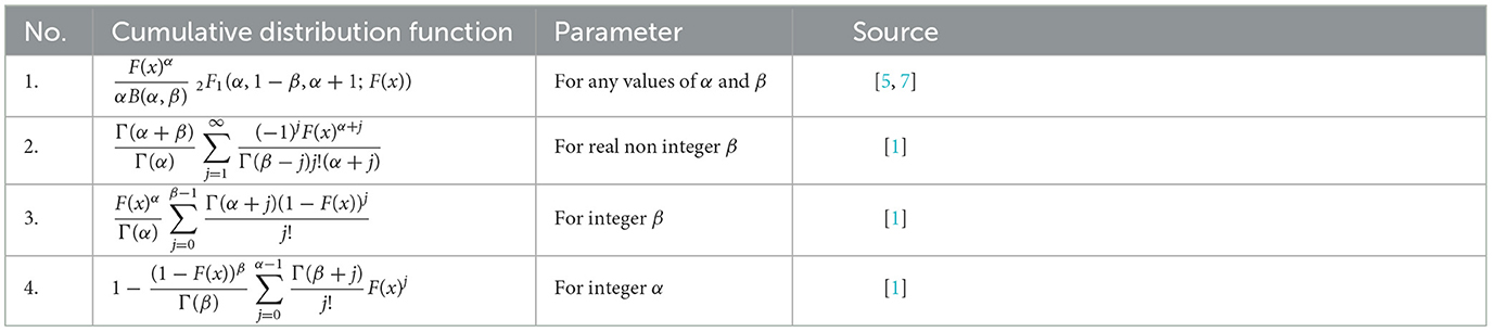
Table 1. Some closed-form expansions for Equation (5) distribution based on real, non-integer, or integer parameters.

Now, by changing variables, let $t=\frac{u}{1-u}$ we get $u=\frac{t}{1+t}$. To change limit of integration from 0 to ∞, consider t → 0, u → 0;t → 1, u → ∞.

Therefore, we have:

$\begin{array}{l}\frac{1}{B\left(\alpha ,\beta \right)}{\displaystyle {\int }_0^1}{u}^{\alpha -1}{\left(1-u\right)}^{\beta -1}du\\ =\frac{1}{B\left(\alpha ,\beta \right)}{\displaystyle {\int }_0^{\infty }}{\left(\frac{t}{1+t}\right)}^{\alpha -1}{\left(1-\frac{t}{1+t}\right)}^{\beta -1}{\left(\frac{1}{1+t}\right)}^{2}dt\\ =\frac{B\left(\alpha ,\beta \right)}{B\left(\alpha ,\beta \right)}=1\end{array}$

Therefore, we have shown that ${\int }_0^{\infty }g\left(x\right)dx=1$

Corollary 1.1. Asymptotic properties:

i. ${lim}_{x\to \infty }G\left(x\right)=1$

ii. ${lim}_{x\to \infty }g\left(x\right)=0$

Proof. To prove (i), the property for the confluent hypergeometric function ₂F₁ from the book [41] is:

$\begin{array}{l}{}_{2}F{}_1(\alpha ,1-\beta ;\alpha +1;1)=\frac{\Gamma (\alpha +1)\Gamma (\beta )}{\Gamma (\alpha +\beta )}\\ \text{ and }\alpha B(\alpha ,\beta )=\frac{\Gamma (\alpha +1)\Gamma (\beta )}{\Gamma (\alpha +\beta )}.\end{array}$

where Γ(·) is the Gamma function and the properties of the beta function, respectively.

Then,

$\begin{array}{l}\underset{x\to \infty }{\lim }G(x)\\ =\underset{x\to \infty }{\lim }\frac{{\left(\frac{1}{2}\mathrm{erfc}\left(\frac{\mu -x}{\sigma \sqrt{2}}\right)-\frac{1}{2}\exp \left(\frac{\lambda }{2}(2\mu +\lambda {\sigma }^2-2x)\right)\mathrm{erfc}\left(\frac{\mu +\lambda {\sigma }^2-x}{\sigma \sqrt{2}}\right)\right)}^{\alpha }}{\alpha B(\alpha ,\beta )}\times \\ {}_{2}F{}_1(\alpha ,1-\beta ,\alpha +1;\frac{1}{2}\mathrm{erfc}\left(\frac{\mu -x}{\sigma \sqrt{2}}\right)\\ -\frac{1}{2}\exp \left(\frac{\lambda }{2}(2\mu +\lambda {\sigma }^2-2x)\right)\mathrm{erfc}\left(\frac{\mu +\lambda {\sigma }^2-x}{\sigma \sqrt{2}}\right))\\ \underset{x\to \infty }{\lim }G(x)=\frac{{\left(1\right)}^{\alpha }}{\alpha B(\alpha ,\beta )}{\times }_2{F}_1\left(\alpha ,1-\beta ,\alpha +1;1\right)\\ =\frac{{}_{2}F{}_1\left(\alpha ,1-\beta ,\alpha +1;1\right)}{\alpha B(\alpha ,\beta )}=1\end{array}$

We have demonstrated conclusively that:

${\displaystyle {lim}_{x\to \infty }}G\left(x\right)=1$

To prove (ii)

$\begin{array}{l}{\displaystyle \underset{x\to \infty }{lim}}g\left(x\right)\\ ={\displaystyle \underset{x\to \infty }{lim}}\frac{1}{B\left(\alpha ,\beta \right)}(\frac{1}{2}erfc\left(\frac{\mu -x}{\sigma \sqrt{2}}\right)-\frac{1}{2}exp\left(\frac{\lambda }{2}\left(2\mu +\lambda {\sigma }^2-2x\right)\right)\\ erfc\left(\frac{\mu +\lambda {\sigma }^2-x}{\sigma \sqrt{2}}\right){)}^{\alpha -1}\\ \times (1-\frac{1}{2}[erfc\left(\frac{\mu -x}{\sigma \sqrt{2}}\right)-exp\left(\frac{\lambda }{2}\left(2\mu +\lambda {\sigma }^2-2x\right)\right)\\ erfc\left(\frac{\mu +\lambda {\sigma }^2-x}{\sigma \sqrt{2}}\right)]{)}^{\beta -1}\\ \times (\frac{\lambda }{2}exp\left(\frac{\lambda }{2}\left(2\mu +\lambda {\sigma }^2-2x\right)\right)erfc\left(\frac{\mu +\lambda {\sigma }^2-x}{\sigma \sqrt{2}}\right))\\ =\frac{1}{B\left(\alpha ,\beta \right)}{\left(\frac{1}{2}\times 2-\frac{1}{2}\times 0\times 2\right)}^{\alpha -1}\times (1-\frac{1}{2}[2-0\times 2]{)}^{\beta -1}\\ \times (\frac{\lambda }{2}\times 0\times 2)=\frac{1}{B\left(\alpha ,\beta \right)}\times 0=0\end{array}$

Therefore, ${lim}_{x\to \infty }g\left(x\right)=0$.

4.1 Special cases

The following are some special cases of the BExG distribution that we examine:

1. When both α = β = 1, the BExG distribution Equation (10) simplifies to the Ex-Gaussian distribution Equation (1). This distribution is characterized by parameters μ, σ, and λ as derived from the study mentioned in Golubev [39].

2. In the scenario where α = β = 1 and λ → ∞, the BExG distribution Equation (10) transforms into the Gaussian distribution. This transformation is described by the parameters μ and σ proposed by the study mentioned in Marmolejo-Ramos et al. [37].

3. When β = 1, the BExG distribution Equation (3.2) reduces to the generalized exponential-Gaussian distribution. This reduction is governed by parameters λ, μ, σ, and α according to the study mentioned in Marmolejo-Ramos et al. [37].

4. In the case where β = 1, λ → ∞, and α≠1, the BExG distribution Equation (6) conforms to the power-normal distribution. This distribution is characterized by parameters μ, σ, and α, as studied by Chen et al. [42] and Marmolejo-Ramos et al. [37].

5 Plots of the probability distribution

In this section, the BExG probability density function (PDF) and cumulative distribution function (CDF) plots in the Figures 1–5 are presented, showcasing various selected parameter values.

Figure 1

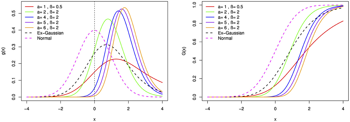
Figure 1. The probability density function (pdf) and cumulative distribution function (cdf) of the BExG distribution are depicted for selected parameter values, with μ = 0, σ = 1, and λ = 1.

Figure 2

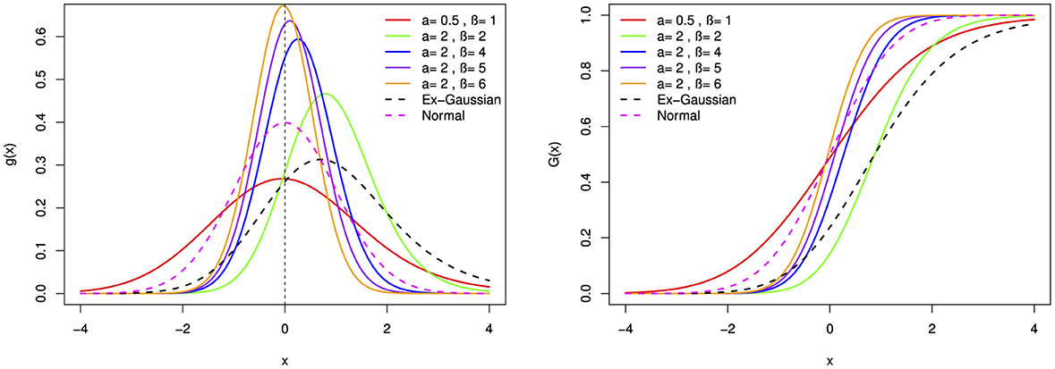
Figure 2. The probability density function (pdf) and cumulative distribution function (cdf) of the BExG distribution are depicted for selected parameter values, with μ = 0, σ = 1, and λ = 1.

Figure 3

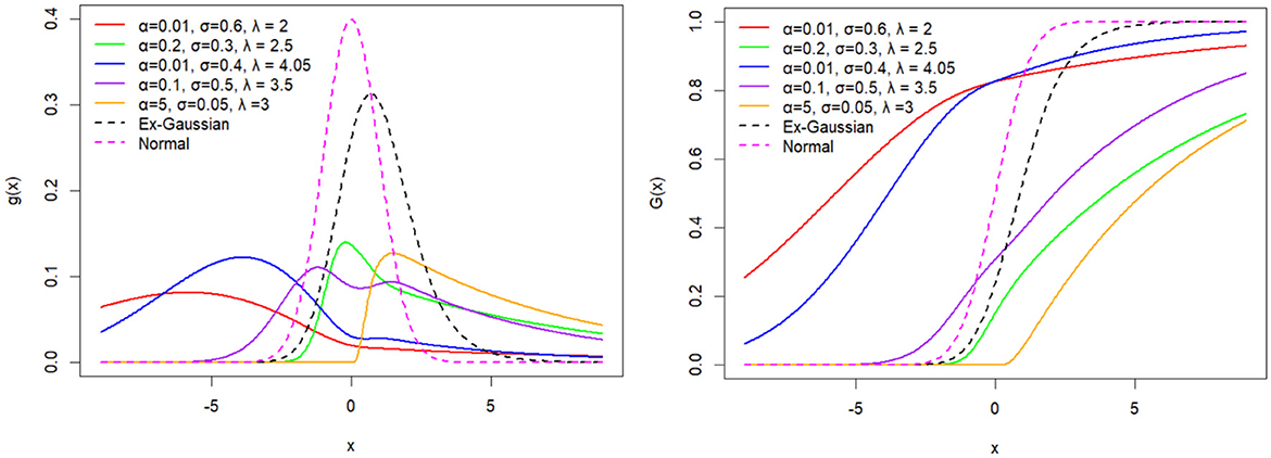
Figure 3. The probability density function (pdf) and cumulative distribution function (cdf) of the BExG distribution are depicted for selected parameter values, with μ = 0 and β = 0.05.

Figure 4

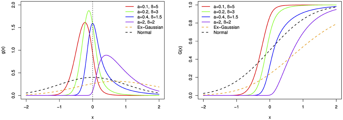
Figure 4. The probability density function (pdf) and cumulative distribution function (cdf) of the BExG distribution are depicted for selected parameter values, with μ = 0, σ = 0.1, and λ = 1.

Figure 5

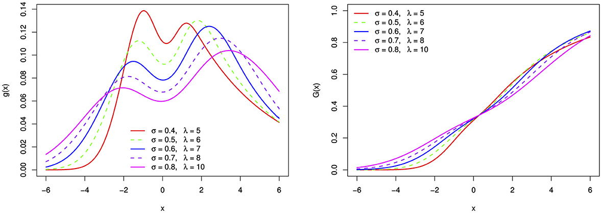
Figure 5. The bimodal probability density function and distribution function of the BExG distribution for selected parameter σ and λ values, with fixed μ = 0, α = 0.1, and β = 0.05.

A bimodal PDF (Figure 5) shows two different peaks or modes, indicating the possibility of two unique processes or sub-populations with various traits. The relative heights of each peak indicate the frequencies and separations between them, while each peak itself represents a mode or cluster within the data.

Some of the shape properties of the uni-modal Beta-Ex-Gaussian distribution include:

• The proposed distribution is a right-skewed distribution when α > β. As α increases with β fixed, the degree of right skewness increases.

• Conversely, the distribution demonstrates left-skewness when α < β. As β increases with α fixed, the degree of left skewness increases.

• Notably, when α≠β, the distribution demonstrates skewness.

• In the case where α = β, the distribution attains symmetry.

• When both α > 1 and β > 1, the distribution is characterized as leptokurtic, exhibiting a higher peak.

• Conversely, when both α < 1 and β < 1, the distribution assumes a platykurtic form, featuring a heavier tail.

• Specifically, when α = 1, β = 1, and λ → ∞, the distribution is categorized as mesokurtic, closely resembling a normal distribution.

In general, the new distribution provides more flexible and versatile shapes that are different from those of normal and exponential-normal distributions.

6 Moments of the Beta-Ex-Gaussian

In probability and statistics, expectations of powers are moments of random variables, where the first is the expectation and the second is the variance, or the second central moment [43].

For β ∈ ℝ\ℤ, we have the power series

$\begin{array}{ll}{\left(1-F\left(x\right)\right)}^{\beta -1}={\displaystyle \sum _{j=0}^{\infty }}{\left(-1\right)}^j\left(\begin{array}{c}\beta -1\\ j\end{array}\right)F{\left(x\right)}^j& (11)\end{array}$

If β ∈ ℤ, the index j in the sum stops at β−1 [7].

For α ∈ ℝ\ℤ, F(x)^α+j−1 can be expanded:

$\begin{array}{l}F{\left(x\right)}^{\alpha +j-1}={\left[1-\left(1-F\left(x\right)\right)\right]}^{\alpha +j-1}\\ ={\displaystyle \sum _{i=0}^{\infty }}{\left(-1\right)}^i\left(\begin{array}{c}\alpha +j-1\\ i\end{array}\right){\left(1-F\left(x\right)\right)}^i\\ ={\displaystyle \sum _{i=0}^{\infty }}{\displaystyle \sum _{r=0}^i}{\left(-1\right)}^{i+r}\left(\begin{array}{c}\alpha +j-1\\ i\end{array}\right)\left(\begin{array}{c}i\\ r\end{array}\right)F{\left(x\right)}^r& (12)\end{array}$

Theorem 2. When α and β are integers, the n^th moment of the Beta-Ex-Gaussian random variable BExG(α, β, μ, σ, λ) is given in the Equation (13) as follows:

$\begin{array}{l}E\left(X^n\right)=\\ \frac{1}{B\left(\alpha ,\beta \right)}{\displaystyle \sum _{j=0}^{\beta -1}}{\left(-1\right)}^j\left(\begin{array}{c}\beta -1\\ j\end{array}\right)\left\{\begin{array}{c}{\displaystyle {\sum }_{k=0}^{\alpha +j-1}}{\left(-1\right)}^k\left(\begin{array}{c}\alpha +j-1\\ k\end{array}\right)I_{n,k}\end{array}\right\}& (13)\end{array}$

where

$I_{n,k}={\displaystyle {\int }_0^{\infty }}{x}^{n}f\left(x\right){\left(1-F\left(x\right)\right)}^{k}dx$

Proof. The book [44] explains that for a random variable X in Lⁿ, the n^th moment, the mean, and the central moment respectively are:

$\begin{array}{l}E\left[X^n\right]=\int x^{n}d{\text{G}}_X\left(x\right)=\int x^n{\text{g}}_X\left(x\right)dx\\ E\left[X\right]=\int x{\text{g}}_X\left(x\right)dx\\ E\left[{\left(X-E\left[X\right]\right)}^n\right]=\int \left[{\left(X-E\left[X\right]\right)}^n\right]{\text{g}}_X\left(x\right)dx\end{array}$

Using Equations (11, 12), and Karr [44] we can prove it as follows:

$\begin{array}{l}E\left[X^n\right]=\int x^{n}d{\text{G}}_X\left(x\right)=\int x^n{\text{g}}_X\left(x\right)dx\\ E\left(X^n\right)={\displaystyle {\int }_0^{\infty }}{x}^n{g}_X\left(x\right)dx\\ \hspace{1em}\hspace{1em}={\displaystyle {\int }_0^{\infty }}{x}^n\frac{1}{B\left(\alpha ,\beta \right)}F{\left(x\right)}^{\alpha -1}{\left[1-F\left(x\right)\right]}^{\beta -1}f\left(x\right)dx\\ \hspace{1em}\hspace{1em}=\frac{1}{B\left(\alpha ,\beta \right)}{\displaystyle \sum _{j=0}^{\beta -1}}{\left(-1\right)}^j\left(\begin{array}{c}\beta -1\\ j\end{array}\right){\displaystyle {\int }_0^{\infty }}{x}^{n}F{\left(x\right)}^{\alpha -1}F{\left(x\right)}^{j}f\left(x\right)dx\\ \hspace{1em}\hspace{1em}=\frac{1}{B\left(\alpha ,\beta \right)}{\displaystyle \sum _{j=0}^{\beta -1}}{\left(-1\right)}^j\left(\begin{array}{c}\beta -1\\ j\end{array}\right){\displaystyle {\int }_0^{\infty }}{x}^{n}F{\left(x\right)}^{\alpha +j-1}f\left(x\right)dx\\ \hspace{1em}\hspace{1em}=\frac{1}{B\left(\alpha ,\beta \right)}{\displaystyle \sum _{j=0}^{\beta -1}}{\left(-1\right)}^j\left(\begin{array}{c}\beta -1\\ j\end{array}\right)\\ {\displaystyle {\int }_0^{\infty }}{x}^n{\left[1-\left(1-F\left(x\right)\right)\right]}^{\alpha +j-1}f\left(x\right)dx\\ \hspace{1em}\hspace{1em}=\frac{1}{B\left(\alpha ,\beta \right)}{\displaystyle \sum _{j=0}^{\beta -1}}{\left(-1\right)}^j\left(\begin{array}{c}\beta -1\\ j\end{array}\right)\\ \left\{\begin{array}{c}\sum _{k=0}^{\alpha +j-1}{\left(-1\right)}^k\left(\begin{array}{c}\alpha +j-1\\ k\end{array}\right)I_{n,k}\end{array}\right\}\end{array}$

where

$I_{n,k}={\displaystyle {\int }_0^{\infty }}{X}^{n}f\left(x\right){\left(1-F\left(x\right)\right)}^{k}dx$

The variance, skewness, and kurtosis measures can be calculated and related using the study mentioned in Jafari et al. [5] and Bury [43] in the Equations (14–16) respectively.

$\begin{array}{ll}Var\left(X\right)=E\left(X^2\right)-E{\left(X\right)}^2& (14)\end{array}$

$\begin{array}{ll}Skewness\left(X\right)=E{\left(\frac{X-\mu }{\sigma }\right)}^3=\frac{E\left(X^3\right)-3E\left(X\right)E\left(X^2\right)+2E{\left(X\right)}^3}{Var{\left(X\right)}^{3/2}}& (15)\end{array}$

$\begin{array}{l}Kurtosis\left(X\right)=E{\left(\frac{X-\mu }{\sigma }\right)}^4\\ =\frac{E\left(X^4\right)-4E\left(X\right)E\left(X^3\right)+6E\left(X^2\right)E{\left(X\right)}^2-3E{\left(X\right)}^4}{Var{\left(X\right)}^2}& (16)\end{array}$

The skewness and kurtosis measures are controlled mainly by the parameters α and β, and Figure 6 illustrates their variation using μ = 0, σ = 1, and λ = 1.

Figure 6

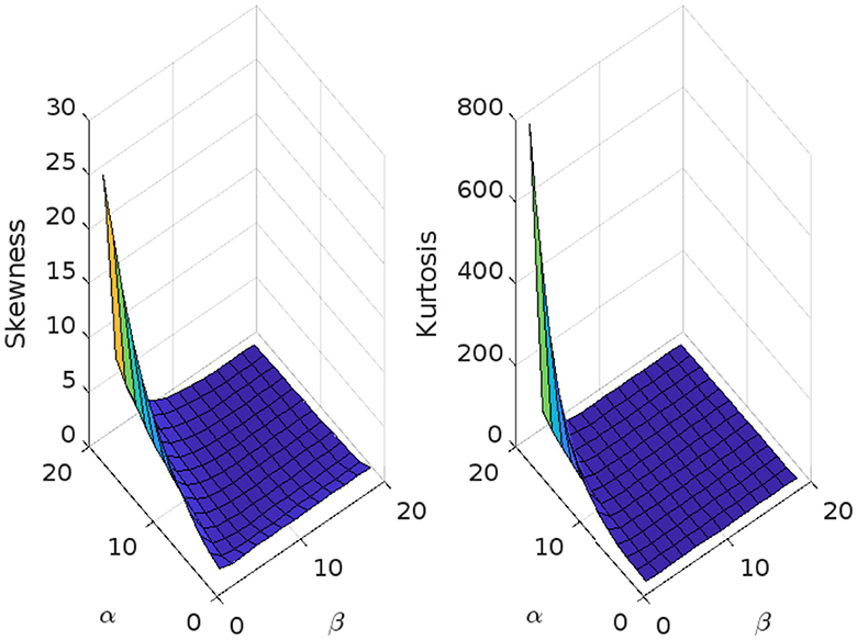
Figure 6. Skewness and kurtosis measures vs. α = 1, 1.5, ⋯ , 20 and β = 1, 1.5, ⋯ , 20 for the beta Ex-Gaussian distribution using μ = 0, σ = 1, and λ = 1.

The skewness and kurtosis measures are controlled mainly by the parameters α and β, and Figures 6–10 illustrates their variation using various parametric values for μ, σ, and λ. More figures are illustrated in Appendix A. The skewness and kurtosis demonstrate strictly increasing, strictly decreasing, and U-shaped behaviors, which are interesting in some applications of the model.

Figure 7

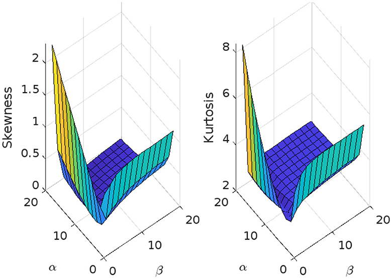
Figure 7. Skewness and kurtosis measures vs. α = 1, 1.5, ⋯ , 20 and β = 1, 1.5, ⋯ , 20 for the beta Ex-Gaussian distribution sing μ = 1, σ = 1, and λ = 1.

Figure 8

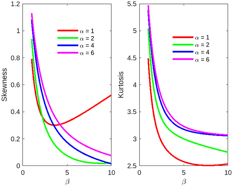
Figure 8. Skewness and kurtosis measures vs. β = 1, 1.5, ⋯ , 10 for the beta Ex-Gaussian distribution: μ = 1, σ = 1, and λ = 1.5.

Figure 9

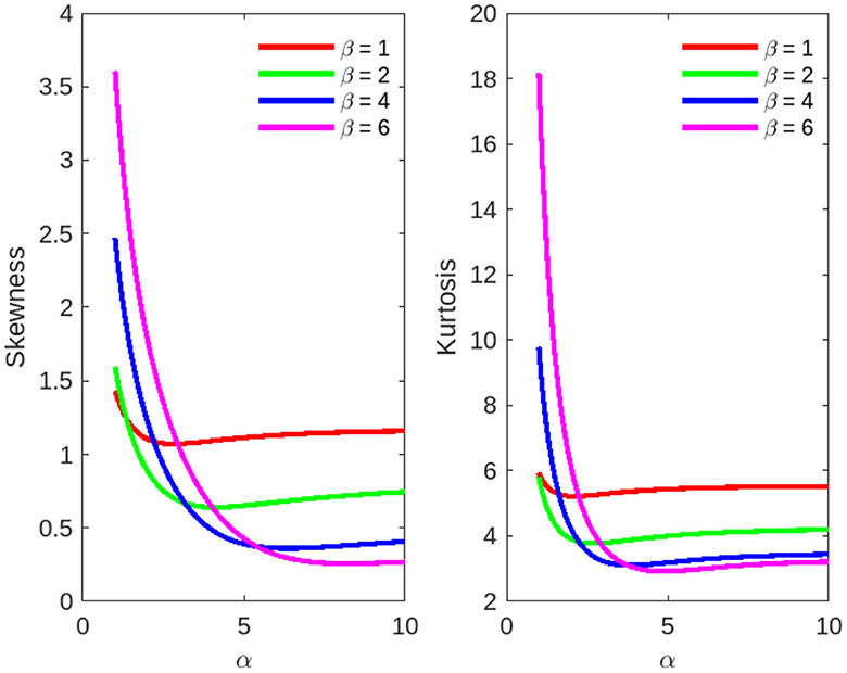
Figure 9. Skewness and kurtosis measures vs. α = 1, 1.5, ⋯ , 10 for the beta Ex-Gaussian distribution.

Figure 10

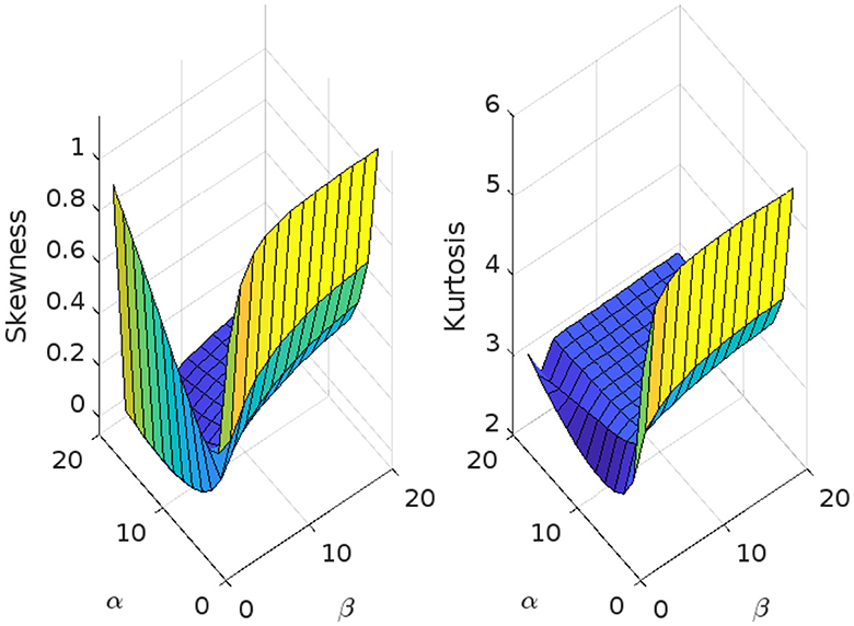
Figure 10. Skewness and kurtosis measures vs. α = 1, 1.5, ⋯ , 20 and β = 1, 1.5, ⋯ , 20 for the beta Ex-Gaussian distribution using μ = 1.5, σ = 1, and λ = 1.

Moreover, Tables 2, 3 illustrate how the mean and median values of a distribution offer insights into its central tendency. Skewness gauges the asymmetry of the distribution, with positive values suggesting longer or fatter right tails and negative values indicating the opposite. Kurtosis, on the other hand, measures the tailedness of the distribution, with higher values indicating heavier tails or more outliers. Additionally, the impact of α on the distribution's skewness and kurtosis can be observed; a higher α value may result in a more asymmetric distribution.

Table 2

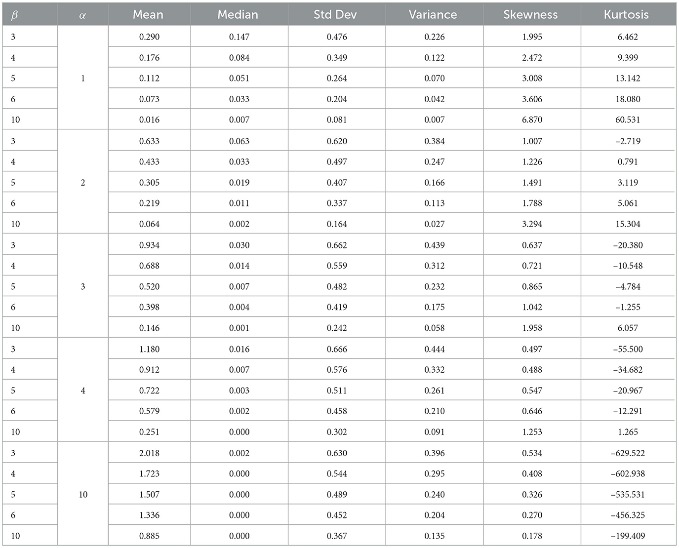
Table 2. The mean, variance, median, standard deviation, skewness, and kurtosis for μ = 0, λ = 1, and σ = 1.

Table 3

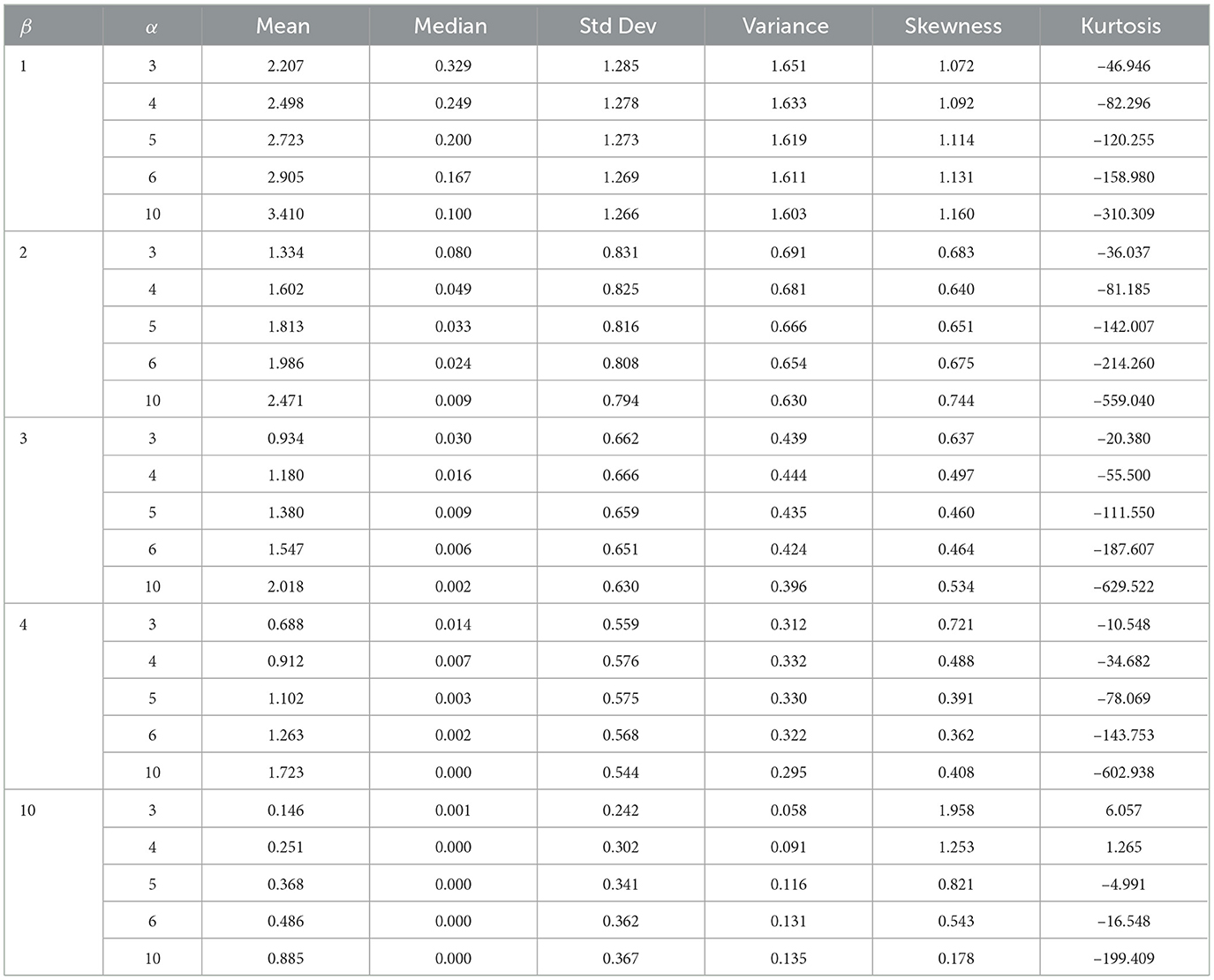
Table 3. The mean, variance, median, standard deviation, skewness, and kurtosis for μ = 0, λ = 1, and σ = 1.

7 Order statistics

The density of the i^th order statistic X_i:n, g_i:n(x) say, in a random sample of size n from the BExG distribution is obtained from the well-known formula [7] is given in the Equation (17) as follows.

$\begin{array}{ll}{g}_{i:n\left(x\right)}=\frac{g_{i:n\left(x\right)}}{B\left(i,n-i+1\right)}G{\left(x\right)}^{i-1}{\left(1-G\left(x\right)\right)}^{n-i}& (17)\end{array}$

Or let X₁, X₂, ..., X_n be a random sample of size n from BExG(μ, σ², λ, α, β). Then the pdf and cdf of the i^th order statistic, say X_i:n, are given by Jafari et al. [5]

$\begin{array}{ll}{g}_{i:n}\left(x\right)=\frac{1}{B\left(i,n-i+1\right)}{\displaystyle \sum _{m=0}^{n-i}}{\left(-1\right)}^m\left(\begin{array}{c}n-i\\ m\end{array}\right)g\left(x\right)G^{i+m-1}\left(x\right)& (18)\end{array}$

$\begin{array}{l}{G}_{i:n}\left(x\right)={\displaystyle {\int }_0^x}{g}_{i:n}\left(t\right)dt\\ =\frac{1}{B\left(i,n-i+1\right)}{\displaystyle \sum _{m=0}^{n-i}}\frac{{\left(-1\right)}^m}{m+i}\left(\begin{array}{c}n-i\\ m\end{array}\right)G^{i+m}\left(x\right)& (19)\end{array}$

respectively, where $G^{i+m}\left(x\right)={\left({\sum }_{r=0}^{\infty }{b}_{r}F{\left(x\right)}^r\right)}^{i+m}$. Here, we use an equation by Gradshteyn and Ryzhik [45] and Jafari et al. [5], for a power series raised to a positive integer n

${\left({\displaystyle \sum _{r=0}^{\infty }}{b}_r{u}^r\right)}^n={\displaystyle \sum _{r=0}^{\infty }}{c}_{n,r}{u}^r$

where the coefficients c_{n, r} (for r = 1, 2, ...) are easily determined from the recurrence Equation (20)

$\begin{array}{ll}{c}_{n,r}={\left(r{b}_0\right)}^{-1}{\displaystyle \sum _{m=1}^r}\left[m\left(n+1\right)-r\right]b_m{c}_{n,r-m}& (20)\end{array}$

where $c_{n,0}=b_0^n$. The coefficient c_{n, r} can be calculated from c_{n, 0}, ..., c_{n, r−1} and hence from the quantities b₀, ..., b_r.

The Equations (18, 19) can be written as follows:

$\begin{array}{l}{g}_{i:n}\left(x\right)=\frac{1}{B\left(i,n-i+1\right)}{\displaystyle {\sum }_{m=0}^{n-i}}{\displaystyle {\sum }_{r=1}^{\infty }}\frac{1}{m+i}{\left(-1\right)}^{m}r{c}_{i+m,r}f\left(x\right)F^{r-1}\left(x\right)\\ G_{i:n}\left(x\right)=\frac{1}{B\left(i,n-i+1\right)}{\displaystyle {\sum }_{m=0}^{n-i}}{\displaystyle {\sum }_{r=0}^{\infty }}\frac{1}{m+i}{\left(-1\right)}^m{c}_{i+m,r}{F}^r\left(x\right)\end{array}$

Therefore, the s^th moment of X_i:n is as follows

$\begin{array}{l}E\left[X_{i:n}^s\right]=\frac{1}{B\left(i,n-i+1\right)}{\displaystyle {\sum }_{m=0}^{n-i}}{\displaystyle {\sum }_{r=1}^{\infty }}\frac{1}{m+i}{\left(-1\right)}^{m}r{c}_{i+m,r}\\ {\displaystyle {\int }_0^{+\infty }}{t}^{s}f\left(t\right)F^{r-1}\left(t\right)dt\end{array}$

which cannot be an explicit expression.

8 Survival and hazard functions

In this section, we refer to Klein and Moeschberger [46] to underscore the fundamental significance of the likelihood of an individual surviving beyond time x as a key metric in characterizing time-to-event events. The survival function, denoted by the random variable X, is described in the Equation (21) as follows (see Klein and Moeschberger [46] for details).

$\begin{array}{ll}S\left(x\right)=P\left(X>x\right)=1-G\left(x\right)& (21)\end{array}$

Furthermore, the hazard function, also referred to as the conditional failure rate, is a critical parameter in survival analysis with broad applications in fields such as economics, epidemiology, demography, and stochastic processes. For a continuous random variable X, the hazard function is defined as follows:

$\begin{array}{ll}h\left(x\right)=\frac{g\left(x\right)}{S\left(x\right)}=\frac{g\left(x\right)}{1-G\left(x\right)}& (22)\end{array}$

Theorem 3. The survival function and hazard function for the new random variable are as follows:

1. Survival function:

$\begin{array}{l}S(x)\\ =1-\frac{{\left(\frac{1}{2}\mathrm{erfc}\left(\frac{\mu -x}{\sigma \sqrt{2}}\right)-\frac{1}{2}\exp \left(\frac{\lambda }{2}(2\mu +\lambda {\sigma }^2-2x)\right)\mathrm{erfc}\left(\frac{\mu +\lambda {\sigma }^2-x}{\sigma \sqrt{2}}\right)\right)}^{\alpha }}{\alpha B(\alpha ,\beta )}\\ \times {}_{2}F{}_1(\alpha ,1-\beta ;\alpha +1;\frac{1}{2}\mathrm{erfc}\left(\frac{\mu -x}{\sigma \sqrt{2}}\right)\\ -\frac{1}{2}\exp \left(\frac{\lambda }{2}(2\mu +\lambda {\sigma }^2-2x)\right)\mathrm{erfc}\left(\frac{\mu +\lambda {\sigma }^2-x}{\sigma \sqrt{2}}\right))& (23)\end{array}$

2. Hazard function:

$\begin{array}{l}h(x)\\ =\frac{\Gamma (\alpha +\beta )}{\Gamma (\alpha )\Gamma (\beta )}{\left(\frac{1}{2}\mathrm{erfc}\left(\frac{\mu -x}{\sigma \sqrt{2}}\right)-\frac{1}{2}\exp \left(\frac{\lambda }{2}(2\mu +\lambda {\sigma }^2-2x)\right)\mathrm{erfc}\left(\frac{\mu +\lambda {\sigma }^2-x}{\sigma \sqrt{2}}\right)\right)}^{\alpha -1}\\ \times {\left(1-\frac{1}{2}\mathrm{erfc}\left(\frac{\mu -x}{\sigma \sqrt{2}}\right)+\frac{1}{2}\exp \left(\frac{\lambda }{2}(2\mu +\lambda {\sigma }^2-2x)\right)\mathrm{erfc}\left(\frac{\mu +\lambda {\sigma }^2-x}{\sigma \sqrt{2}}\right)\right)}^{\beta -1}\\ \times \left(\frac{\lambda }{2}\exp \left(\frac{\lambda }{2}(2\mu +\lambda {\sigma }^2-2x)\right)\text{erfc}\left(\frac{\mu +\lambda {\sigma }^2-x}{\sigma \sqrt{2}}\right)\right)\\ \times (1-\frac{\Gamma (\alpha +\beta ){\left(\frac{1}{2}\mathrm{erfc}\left(\frac{\mu -x}{\sigma \sqrt{2}}\right)-\frac{1}{2}\exp \left(\frac{\lambda }{2}(2\mu +\lambda {\sigma }^2-2x)\right)\mathrm{erfc}\left(\frac{\mu +\lambda {\sigma }^2-x}{\sigma \sqrt{2}}\right)\right)}^{\alpha }}{\alpha \Gamma (\alpha )\Gamma (\beta )}\\ \times {}_{2}F{}_1(\alpha ,1-\beta ;\alpha +1;\frac{1}{2}\mathrm{erfc}\left(\frac{\mu -x}{\sigma \sqrt{2}}\right)-\frac{1}{2}\exp \left(\frac{\lambda }{2}(2\mu +\lambda {\sigma }^2-2x)\right)\\ {\mathrm{erfc}\left(\frac{\mu +\lambda {\sigma }^2-x}{\sigma \sqrt{2}}\right)))}^{-1}& (24)\end{array}$

Proof. Equations (21, 22) can be used to easily obtain the proof for Equations (23, 24), respectively.

Corollary 3.1. Asymptotic behaviors:

${lim}_{x\to \infty }S\left(x\right)=0$

Proof.

$\begin{array}{c}\underset{x\to \infty }{\lim }S(x)\\ =\underset{x\to \infty }{\lim }(1-\frac{{\left(\frac{1}{2}\mathrm{erfc}\left(\frac{\mu -x}{\sigma \sqrt{2}}\right)-\frac{1}{2}\exp \left(\frac{\lambda }{2}(2\mu +\lambda {\sigma }^2-2x)\right)\mathrm{erfc}\left(\frac{\mu +\lambda {\sigma }^2-x}{\sigma \sqrt{2}}\right)\right)}^{\alpha }}{\alpha B(\alpha ,\beta )}\times \\ {}_{2}F{}_1\left(\alpha ,1-\beta ;\alpha +1;\frac{1}{2}\mathrm{erfc}\left(\frac{\mu -x}{\sigma \sqrt{2}}\right)-\frac{1}{2}\exp \left(\frac{\lambda }{2}(2\mu +\lambda {\sigma }^2-2x)\right)\mathrm{erfc}\left(\frac{\mu +\lambda {\sigma }^2-x}{\sigma \sqrt{2}}\right)\right))\\ =1-\frac{{\left(\frac{1}{2}\mathrm{erfc}\left(\frac{\mu -\infty }{\sigma \sqrt{2}}\right)-\frac{1}{2}\exp \left(\frac{\lambda }{2}(2\mu +\lambda {\sigma }^2-\infty )\right)\mathrm{erfc}\left(\frac{\mu +\lambda {\sigma }^2-\infty }{\sigma \sqrt{2}}\right)\right)}^{\alpha }}{\alpha B(\alpha ,\beta )}\\ \times {}_{2}F{}_1\left(\alpha ,1-\beta ;\alpha +1;\frac{1}{2}\mathrm{erfc}\left(\frac{\mu -\infty }{\sigma \sqrt{2}}\right)-\frac{1}{2}\exp \left(\frac{\lambda }{2}(2\mu +\lambda {\sigma }^2-\infty )\right)\mathrm{erfc}\left(\frac{\mu +\lambda {\sigma }^2-\infty }{\sigma \sqrt{2}}\right)\right)\\ =1-\frac{{\left(\frac{1}{2}\mathrm{erfc}\left(-\infty \right)-\frac{1}{2}\exp \left(-\infty \right)\mathrm{erfc}\left(-\infty \right)\right)}^{\alpha }}{\alpha B(\alpha ,\beta )}\\ \times {}_{2}F{}_1\left(\alpha ,1-\beta ;\alpha +1;\frac{1}{2}\mathrm{erfc}\left(-\infty \right)-\frac{1}{2}\exp \left(-\infty )\right)\mathrm{erfc}\left(-\infty \right)\right)\\ =1-\frac{{\left(\frac{1}{2}\times 2-\frac{1}{2}\times 0\times 2\right)}^{\alpha }}{\alpha B(\alpha ,\beta )}\times {}_{2}F{}_1\left(\alpha ,1-\beta ;\alpha +1;\frac{1}{2}\times 2-\frac{1}{2}\times 0\times 2\right)\\ =1-\frac{{}_{2}F{}_1\left(\alpha ,1-\beta ;\alpha +1;1\right)}{\alpha B(\alpha ,\beta )}=0\end{array}$

Therefore, ${lim}_{x\to \infty }S\left(x\right)=0$.

Here, we establish a series of plots to visually represent the hazards and survival functions of the BExG distribution. This distribution is characterized by varying parameter values, including α, β, μ, σ, and λ. Through these plots, we aim to provide insights into the probability density and hazards associated with the random variable under consideration.

Based on parameter values, the hazard function can take on a variety of shapes, including monotonically increasing, decreasing, bimodal, parabolas, and bumping shapes. The hazard rate function appears to converge to a fixed value over a large range of x. Figures 11–16 reveal that larger α and β values result in higher hazard rates compared with those of the base distribution. Overall, the new distribution manifests shapes and patterns that are distinct from the base distribution. Specifically, the shape parameters play a crucial role in generating the interesting shapes observed in the new BExG probability distribution. The instantaneous rate of an event of interest is described by a bimodal hazard function, where each peak denotes a higher risk period.

Figure 11

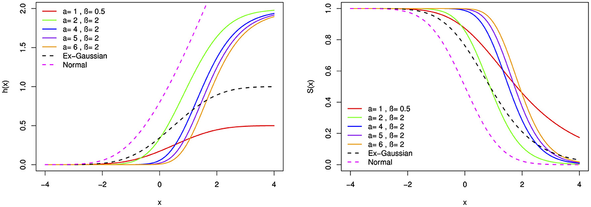
Figure 11. The hazard function (h(x)) and survival function (S(x)) of the BExG distribution are depicted for selected parameter values, with μ = 0, σ = 1, and λ = 1.

Figure 12

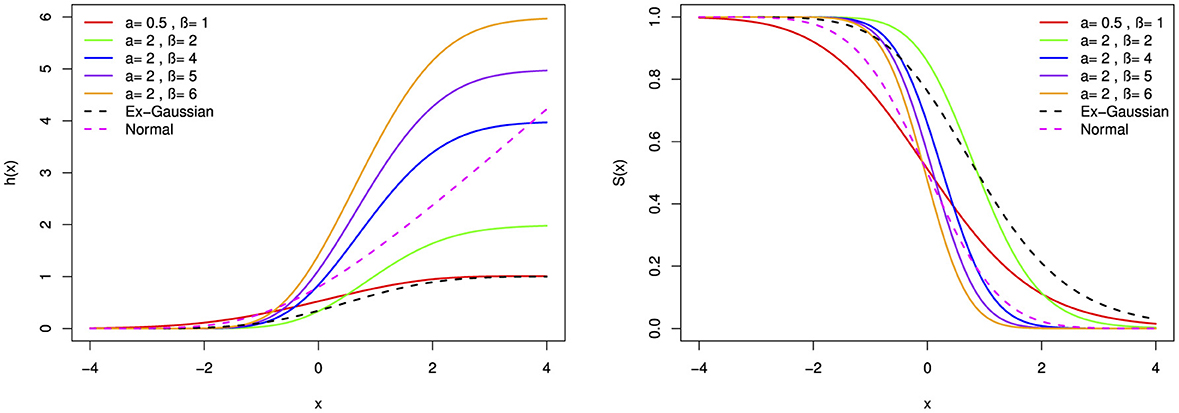
Figure 12. The hazard function (h(x)) and survival function (S(x)) of the BExG distribution are depicted for selected parameter values, with μ = 0 and β = 0.05.

Figure 13

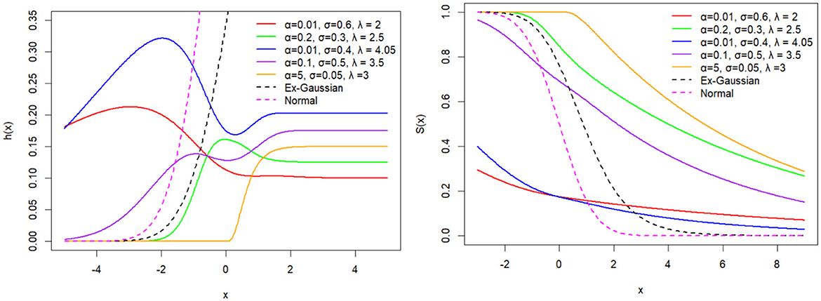
Figure 13. The hazard function (h(x)) and survival function (S(x)) of the BExG distribution are depicted for selected parameter values, with μ = 0 and β = 0.05.

Figure 14

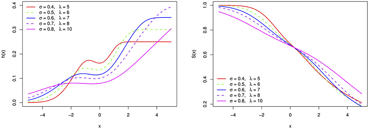
Figure 14. The bimodal hazard function (h(x)) and survival function (S(x)) of the BExG distribution are depicted for selected parameter values, with μ = 0, β = 0.05, and α = 0.1.

Figure 15

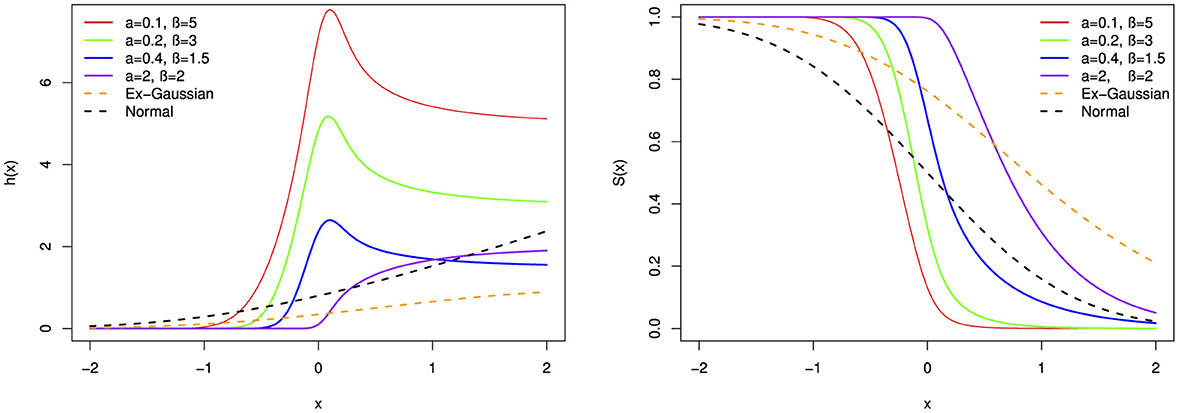
Figure 15. The hazard function (h(x)) and survival function (S(x)) of the BExG distribution are depicted for selected parameter values, with μ = 0, σ = 0.1, and λ = 1.

Figure 16

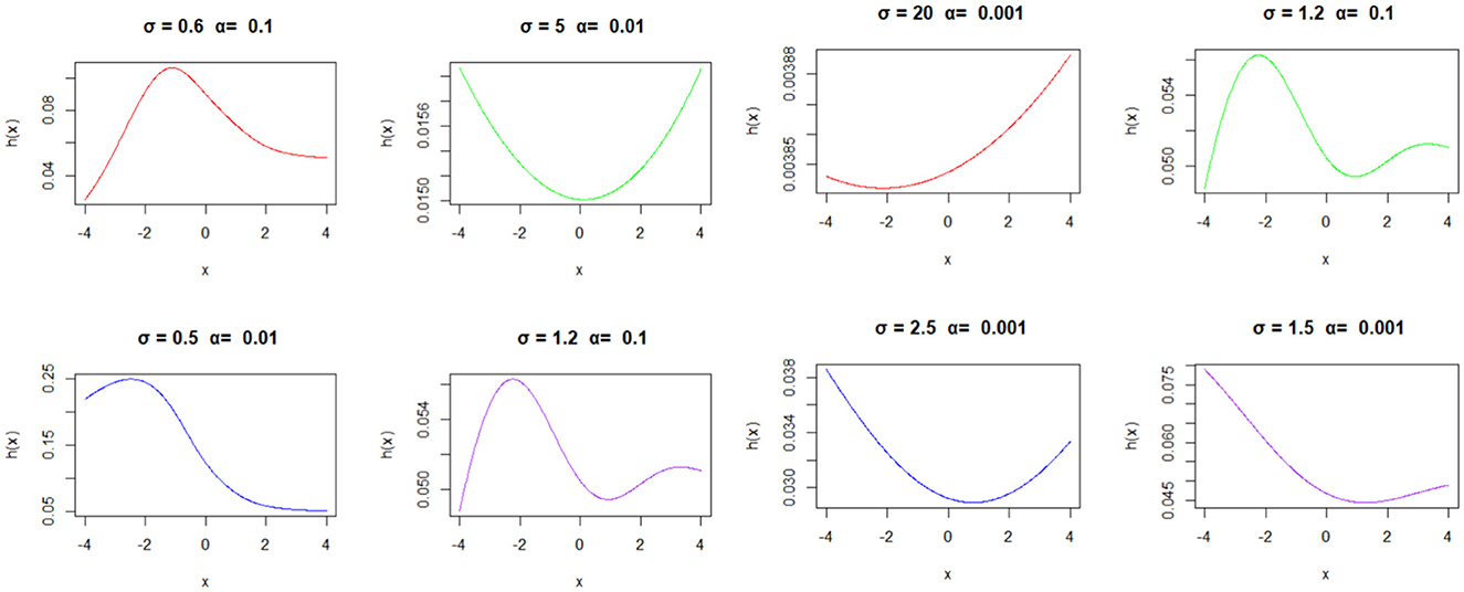
Figure 16. The BExG distribution's hazard functions are depicted in various subplots, each representing a different combination of parameters (σ and α), providing valuable insights into the associated random variable, with β = 0.05, μ = 0, and λ = 1.

Now, we go into the analysis of specific hazard function plots (Figure 16) derived from the BExG distribution across a range of parameter values, with particular attention to the scale (σ) and shape (α) parameters. Our aim is to elucidate their influence on the hazard profiles of the distribution and their implications for practical applications.

9 Parameter estimation

Let X₁, X₂, ⋯ , X_n be n i.i.d. random observations generated from the new distribution g(x; Φ).

The likelihood and log-likelihood function for the new BExG distribution are given by Equations (25, 26), respectively.

$\begin{array}{ll}L\left(\Phi |x\right)=L\left(\alpha ,\beta ,\mu ,\sigma ,\lambda |x\right)={\displaystyle {\prod }_{i=1}^n}g\left(x_i|\alpha ,\beta ,\mu ,\sigma ,\lambda \right)& (25)\end{array}$

$\begin{array}{l}\ell \left(\Phi |x\right)=\left(\alpha -1\right){\displaystyle {\sum }_{i=1}^n}ln(\frac{1}{2}erfc\left(\frac{\mu -x_i}{\sigma \sqrt{2}}\right)\\ \hspace{1em}\hspace{1em}-\frac{1}{2}exp\left(\frac{\lambda }{2}\left(2\mu +\lambda {\sigma }^2-2x_i\right)\right)erfc\left(\frac{\mu +\lambda {\sigma }^2-x_i}{\sigma \sqrt{2}}\right))\\ \hspace{1em}\hspace{1em}+\left(\beta -1\right){\displaystyle {\sum }_{i=1}^n}ln(1-\frac{1}{2}erfc\left(\frac{\mu -x_i}{\sigma \sqrt{2}}\right)\\ \hspace{1em}\hspace{1em}+\frac{1}{2}exp\left(\frac{\lambda }{2}\left(2\mu +\lambda {\sigma }^2-2x_i\right)\right)erfc\left(\frac{\mu +\lambda {\sigma }^2-x_i}{\sigma \sqrt{2}}\right))\\ \hspace{1em}\hspace{1em}+{\displaystyle {\sum }_{i=1}^n}ln(\frac{\lambda }{2}exp\left(\frac{\lambda }{2}\left(2\mu +\lambda {\sigma }^2-2x_i\right)\right)\\ \hspace{1em}\hspace{1em}\text{erfc}\left(\frac{\mu +\lambda {\sigma }^2-x_i}{\sigma \sqrt{2}}\right))-nlnB\left(\alpha ,\beta \right)& (26)\end{array}$

Here, Φ = {α, β, μ, σ, λ}.

The Maximum Likelihood Estimate (MLE), denoted as $\widehat{\Phi }$ or $\widehat{\alpha },\widehat{\beta },\widehat{\sigma },\widehat{\lambda }$, is the set of parameter values, which maximizes the likelihood function or, equivalently, the log-likelihood function [47]

$\widehat{\Phi }=arg{\displaystyle \underset{\Phi \in \Omega }{max}}L\left(\Phi |x\right)=arg{\displaystyle \underset{\Phi \in \Omega }{max}}\ell \left(\Phi |X\right)$

Let Φ = {α, β, μ, σ, λ} and the log-likelihood function be denoted as ℓ(Φ|x).

The Maximum Likelihood Estimator (MLE) for each parameter is obtained by taking partial derivatives of the log-likelihood function and setting the equation equal to zero. i.e.,

$\begin{array}{l}\widehat{\Phi }=\{\begin{array}{c}\widehat{\alpha }=\frac{\partial \ell }{\partial \alpha }={\displaystyle {\sum }_{i=1}^n}\frac{\partial ln\left(g\left(x_i|\alpha ,\beta ,\mu ,\sigma ,\lambda \right)\right)}{\partial \alpha }=0\\ \widehat{\beta }=\frac{\partial \ell }{\partial \beta }={\displaystyle {\sum }_{i=1}^n}\frac{\partial ln\left(g\left(x_i|\alpha ,\beta ,\mu ,\sigma ,\lambda \right)\right)}{\partial \beta }=0\\ \widehat{\mu }=\frac{\partial \ell }{\partial \mu }={\displaystyle {\sum }_{i=1}^n}\frac{\partial ln\left(g\left(x_i|\alpha ,\beta ,\mu ,\sigma ,\lambda \right)\right)}{\partial \mu }=0\\ \widehat{\sigma }=\frac{\partial \ell }{\partial \sigma }={\displaystyle {\sum }_{i=1}^n}\frac{\partial ln\left(g\left(x_i|\alpha ,\beta ,\mu ,\sigma ,\lambda \right)\right)}{\partial \sigma }=0\\ \widehat{\lambda }=\frac{\partial \ell }{\partial \lambda }={\displaystyle {\sum }_{i=1}^n}\frac{\partial ln\left(g\left(x_i|\alpha ,\beta ,\mu ,\sigma ,\lambda \right)\right)}{\partial \lambda }=0\end{array}\end{array}$

Since it was not easy to determine the estimated parameters analytically, we used numerical optimization approaches.

10 Simulations

This section explores the use of the acceptance-rejection algorithm, a fundamental method in statistical simulation used to produce random samples from probability distributions that are difficult to sample directly. In particular, we study the Beta-Ex-Gaussian (BExG) distribution, which is a probabilistic complex that combines elements of the beta, exponential, and Gaussian distributions. The most important steps in the acceptance-rejection algorithm by the study mentioned in Robert and Casella [48] are as follows:

Step 1. Generate a random variable Y from a proposal density function g(y).

Step 2. Generate a uniform random variable, U, which is independent of Y.

Step 3. If $U\le \frac{f\left(y\right)}{Mg\left(y\right)}$, accept the proposed Y and set X = Y; otherwise, go to step 1.

where g(y) is a known distribution close to f(y), and M is a constant number that is the upper bound such that $\frac{f\left(y\right)}{g\left(y\right)}<M$. In our case, f(y) is the new Beta-Ex-Gaussian density function.

The simulation involves generating N = 10,000 samples from the target distribution. Subsequently, the algorithm visually presents the simulated samples through density plots and histograms to illustrate their distribution, as illustrated in Figures 17–19. The histograms show that the distribution can be skewed distribution depending on the parameter values.

Figure 17

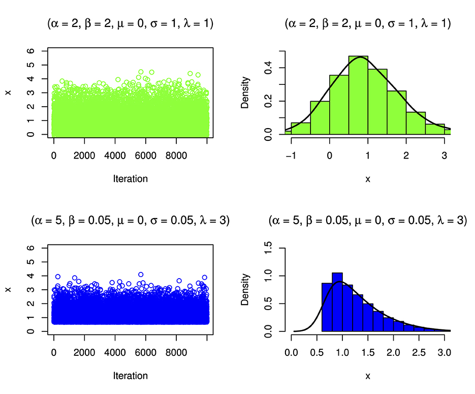
Figure 17. Simulated distribution and its corresponding density estimate for a case of the BExG distribution with specific parameters.

Figure 18

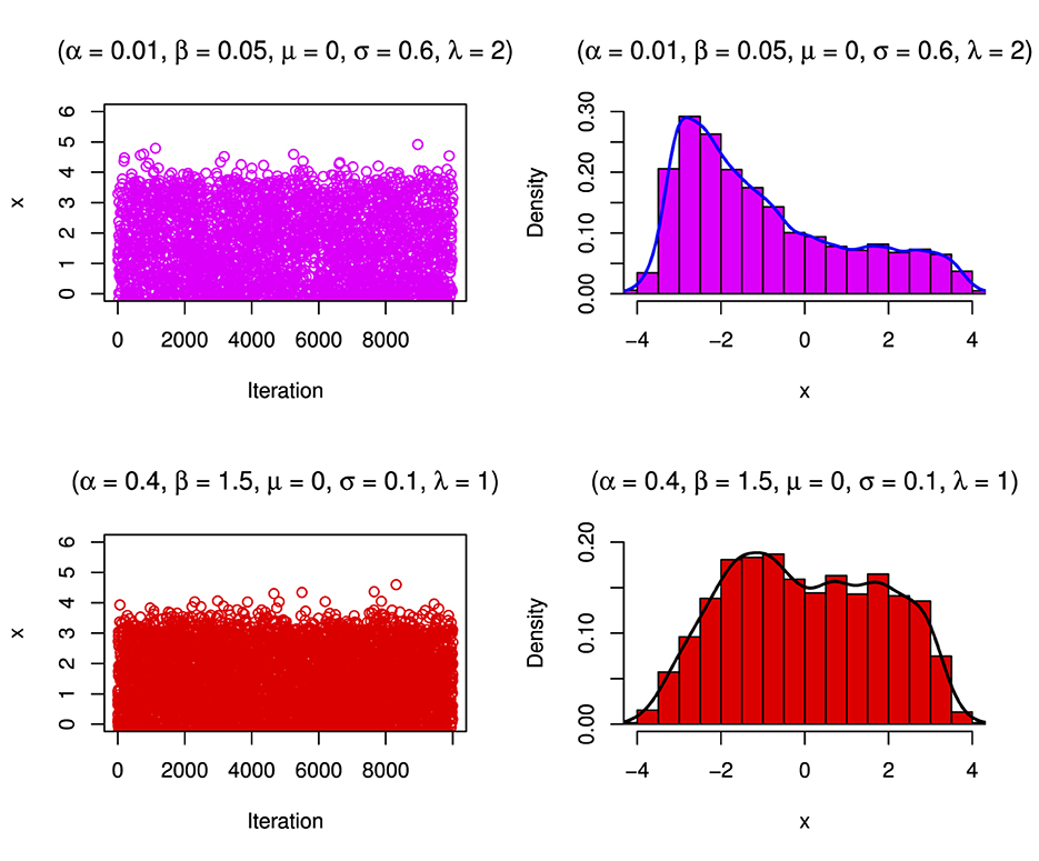
Figure 18. Simulated distribution and its corresponding density estimate for a case of the BExG distribution with specific parameters.

Figure 19

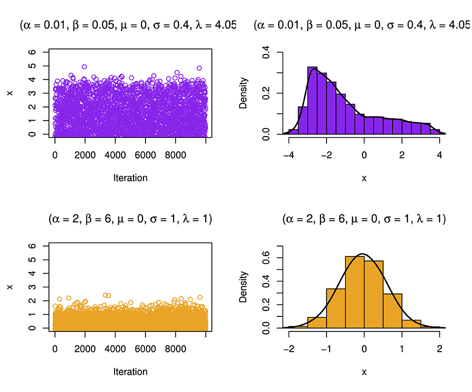
Figure 19. Simulated distribution and its corresponding density estimate for a case of the BExG distribution with specific parameters.

To assess the effectiveness of Maximum Likelihood Estimators (MLEs) for the parameters of the Beta-Ex-Gaussian (BExG) distribution, we conduct simulations across varying sample sizes. The evaluation encompasses three distinct cases characterized by the true parameter sets denoted as Φ_true = (α, β, μ, σ, λ):

• Case I: α = 2, β = 2, μ = 0, σ = 1, λ = 1,

• Case II: α = 5, β = 2, μ = 0, σ = 1, λ = 1, and

• Case III: α = 2, β = 6, μ = 0, σ = 1, λ = 1

The MLE, $\widehat{\Phi }$ for each parameter can be evaluated using two accuracy measures: the bias and the mean square error (MSE).

Table 4 shows biases, MSE, and MLE for simulated data. Larger sample sizes indicate closer convergence toward true parameter values, while lower MSE values indicate better estimation accuracy. Bias represents systematic estimation method overestimation or underestimation, while MSE measures estimator accuracy. In general, from Table 4, we find that the randomness of the sample size affects the fluctuation estimation accuracy, MSE, and bias of model parameters.

Table 4

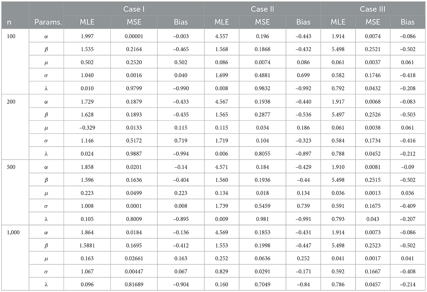
Table 4. Maximum likelihood estimates (MLE), mean squared errors (MSE), and bias of simulated data across different sample sizes and cases.

In our study, a simulated dataset to evaluate the goodness-of-fit of the Beta-Ex-Gaussian distribution using various metrics. The results showed that the new proposed distribution fits better than its base Ex-Gaussian distribution, as shown in Table 5 and Figure 20.

Table 5

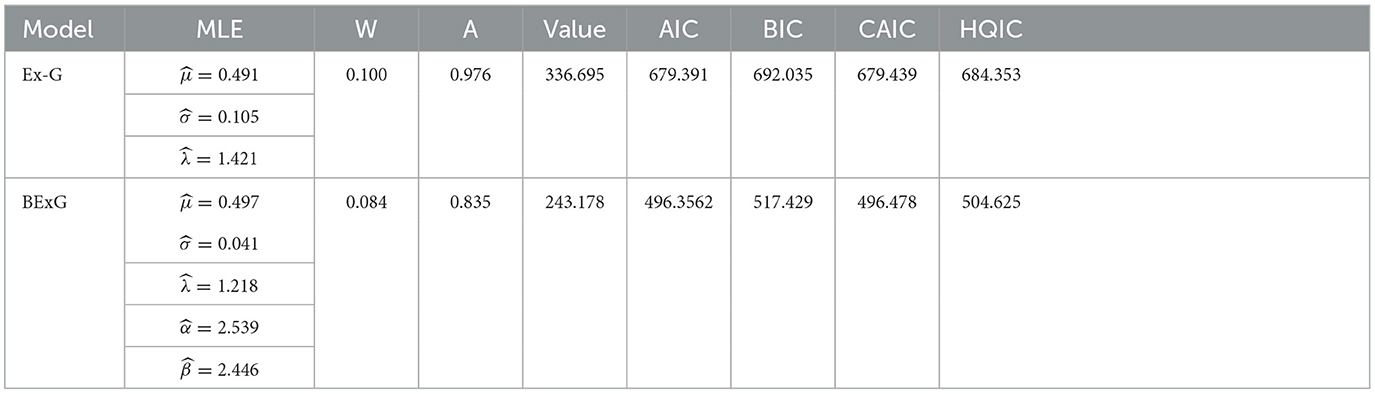
Table 5. The ML estimates, W, A, log-likelihood, BIC, AIC, and CAIC for simulated data.

Figure 20

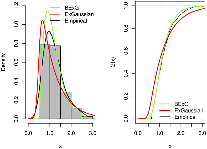
Figure 20. Plots (density and distribution) of fitted BExG and Ex-Gaussian distributions for the simulated data.

11 Applications

In this part, we analyze four actual data sets to demonstrate that the Beta-Ex-Gaussian (BExG) distribution fits better than the Ex-Gaussian (Ex-G) distribution.

To test, measures of goodness-of-fit can be applied in comparison to some other models. Mainly, we use Log-likelihood, statistic Cramer-von misses (W), statistic Anderson Darling (A), Akaike information criterion (AIC), the corrected Akaike information criterion (CAIC), Bayesian information criterion (BIC), and HannanQuinn information criterion (HQIC).

Data set 1: plasma concentrations-Indometh data

The Indometh data, a set of pharmacokinetic data from plasma concentrations of the indometacin vector, is an R-built-in data frame used in our study as data set 1 and is given as follows:

1.5, 0.94, 0.78, 0.48, 0.37, 0.19, 0.12, 0.11, 0.08, 0.07, 0.05, 2.03, 1.63, 0.71, 0.7, 0.64, 0.36, 0.32, 0.2, 0.25, 0.12, 0.08, 2.72, 1.49, 1.16, 0.8, 0.8, 0.39, 0.22, 0.12, 0.11, 0.08, 0.08, 1.85, 1.39, 1.02, 0.89, 0.59, 0.4, 0.16, 0.11, 0.1, 0.07, 0.07, 2.05, 1.04, 0.81, 0.39, 0.3, 0.23, 0.13, 0.11, 0.08, 0.1, 0.06, 2.31, 1.44, 1.03, 0.84, 0.64, 0.42, 0.24, 0.17, 0.13, 0.1, and 0.09.

Data set 2: carbon fiber data

Data set 2 consists of observations on the breaking stress of carbon fibers. The data set that was studied was used by the study mentioned in Kuttan Pillai et al. [49] to study a new generalization of Pareto distribution and its applications. We fit to this data into the new model, BExG and Ex-Gaussian, and compare the results.

3.70 2.74 2.73 2.50 3.60 3.11 3.27 2.87 1.47 3.11 4.42 2.41 3.19 3.22 1.69 3.28 3.09 1.87 3.15 4.90 3.75 2.43 2.95 2.97 3.39 2.96 2.53 2.67 2.93 3.22 3.39 2.81 4.20 3.33 2.55 3.31 3.31 2.85 2.56 3.56 3.15 2.35 2.55 2.59 2.38 2.81 2.77 2.17 2.83 1.92 1.41 3.68 2.97 1.36 0.98 2.76 4.91 3.68 1.84 1.59 3.19 1.57 0.81 5.56 1.73 1.59 2.00 1.22 1.12 1.71 2.17 1.17 5.08 2.48 1.18 3.51 2.17 1.69 1.25 4.38 1.84 0.39 3.68 2.48 0.85 1.61 2.79 4.70 2.03 1.80 1.57 1.08 2.03 1.61 2.12 1.89 2.88 2.82 2.05 3.65.

Data set 3: survival times (in days) of 72 guinea pigs

Data on the survival times (in days) of 72 guinea pigs infected with virulent tubercle bacilli, observed, reported, and used by the study mentioned in Mukherjee et al. [50] to study estimators of the PDF and CDF of the one-parameter polynomial exponential distribution.

0.1, 0.33, 0.44, 0.56, 0.59, 0.72, 0.74, 0.77, 0.92, 0.93, 0.96, 1, 1, 1.02, 1.05, 1.07, 1.07, 1.08, 1.08, 1.08, 1.09, 1.12, 1.13, 1.15, 1.16, 1.2, 1.21, 1.22, 1.22, 1.24, 1.3, 1.34, 1.36, 1.39, 1.44, 1.46, 1.53, 1.59, 1.6, 1.63, 1.63, 1.68, 1.71, 1.72, 1.76, 1.83, 1.95, 1.96, 1.97, 2.02, 2.13, 2.15, 2.16, 2.22, 2.3, 2.31, 2.4, 2.45, 2.51, 2.53, 2.54, 2.54, 2.78, 2.93, 3.27, 3.42, 3.47, 3.61, 4.02, 4.32, 4.58, and 5.55.

Data set 4: Kevlar 49/epoxy strand failure time data (pressure at 90%)

Life data set that displays the stress rupture life in hours of Kevlar 49/epoxy strands under continuous, sustained stress level pressure until failure. The data set has been previously used in the study mentioned in Al-Aqtash et al. [51] to illustrate the usefulness of the Gumbel–Weibull distribution (GWD) when compared with the exponentiated-Weibull, beta normal, and generalized half normal. 0.01, 0.01, 0.02, 0.02, 0.02, 0.03, 0.03, 0.04, 0.05, 0.06, 0.07, 0.07, 0.08, 0.09, 0.09, 0.10, 0.10, 0.11, 0.11, 0.12, 0.13, 0.18, 0.19, 0.20, 0.23, 0.24, 0.24, 0.29, 0.34, 0.35, 0.36, 0.38, 0.40, 0.42, 0.43, 0.52, 0.54, 0.56, 0.60, 0.60, 0.63, 0.65, 0.67, 0.68, 0.72, 0.72, 0.72, 0.73, 0.79, 0.79, 0.80, 0.80, 0.83, 0.85, 0.90, 0.92, 0.95, 0.99, 1.00, 1.01, 1.02, 1.03, 1.05, 1.10, 1.10, 1.11, 1.15, 1.18, 1.20, 1.29, 1.31, 1.33, 1.34, 1.40, 1.43, 1.45, 1.50, 1.51, 1.52, 1.53, 1.54, 1.54, 1.55, 1.58, 1.60, 1.63, 1.64, 1.80, 1.80, 1.81, 2.02, 2.05, 2.14, 2.17, 2.33, 3.03, 3.03, 3.34, 4.20, 4.69, and 7.89.

The BExG distribution yields the smallest values of W, A, Log-likelihood function, AIC, BIC, CAIC, and HQIC statistics, as shown in Tables 6–9. Based on these statistics, it can be concluded that the BExG model outperforms the Ex-Gaussian distribution in fitting the data. The plots of the densities (alongside the data histogram) and cumulative distribution functions (with an empirical distribution function) are provided in Appendix B. These plots demonstrate also that the BExG model offers a superior fit compared with the Ex-Gaussian model.

Table 6

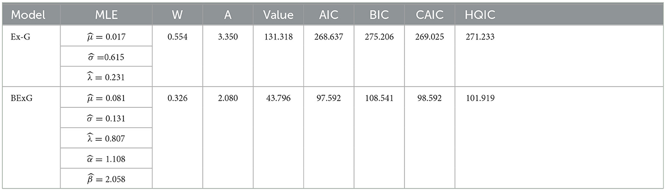
Table 6. MLEs, W, A, log-likelihood, BIC, AIC, and CAIC for data set 1.

Table 7

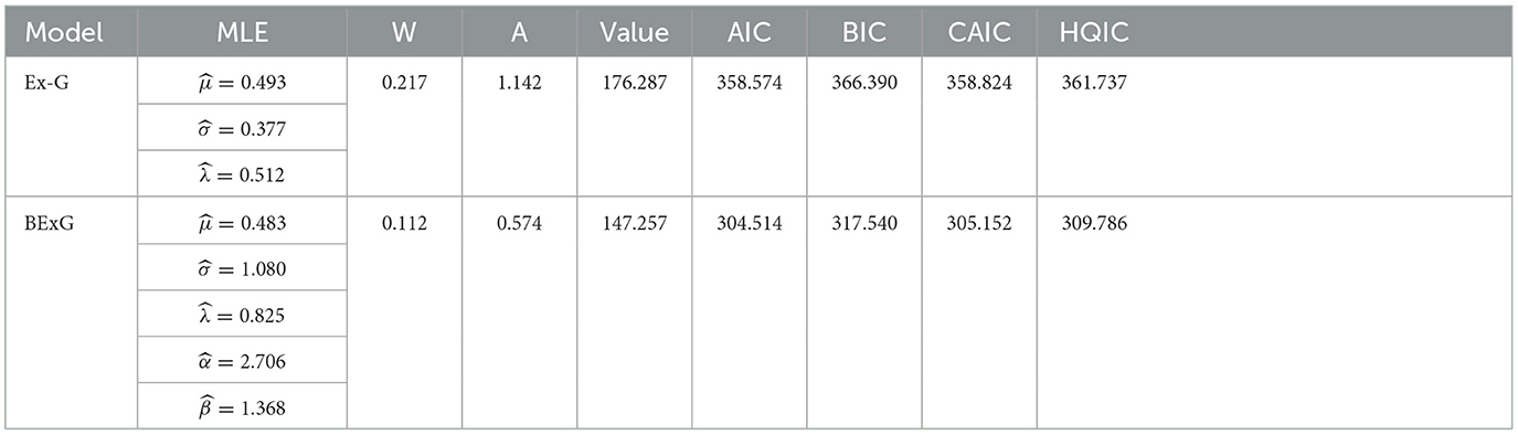
Table 7. MLEs, W, A, log-likelihood, BIC, AIC, and CAIC for data set 2.

Table 8

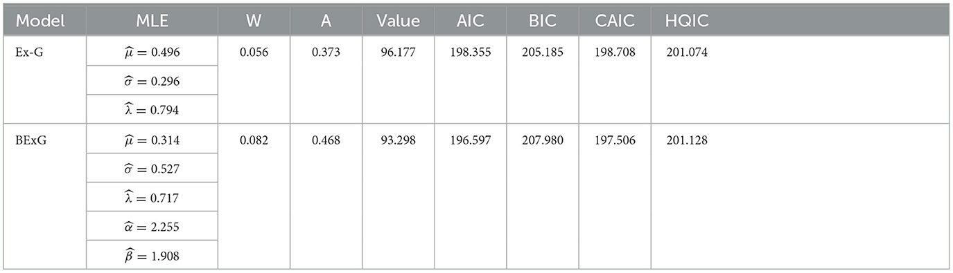
Table 8. MLEs, W, A, log-likelihood, BIC, AIC, and CAIC for data set 3.

Table 9

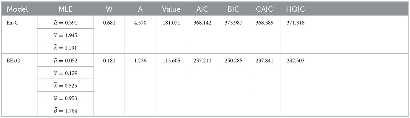
Table 9. MLEs, W, A, log-likelihood, BIC, AIC, and CAIC for data set 4.

12 Conclusion

The aim of this study is to develop a new five-parameter continuous probability distribution, named the Beta-Exponential-Gaussian (BExG) distribution using the method of beta generator. The BExG distribution includes Ex-Gaussian, generalized Ex-Gaussian, normal, and power-normal probability distributions as special cases. It is a new contribution to the Statistical and Probability theory. The research contributes to enhancing modeling capabilities of the base Exponential-Gaussian distribution by proposing the new Beta Exponential-Gaussian distribution which is found to be a promising alternative for data analysis in different application areas including survival and reliability. The basic properties of the new distribution, including reliability measure, hazard function, survival function, moment, skewness, kurtosis, order statistics, and asymptotic behavior, are established. The acceptance-rejection algorithm for simulation is presented. The new model is fitted to the simulated and real data sets, and its performance is revealed. The distribution can model data sets having a distributional nature of various skewness, kurtosis, heavier tails, uni-model, bi-modal, and asymmetric properties. The Beta-Exponential-Gaussian distribution is found to be more flexible, and so, we recommend it to be used for applications.

Data availability statement

The original contributions presented in the study are included in the article/Supplementary material, further inquiries can be directed to the corresponding author.

Author contributions

KT: Conceptualization, Data curation, Formal analysis, Investigation, Methodology, Writing – original draft, Writing – review & editing. AG: Formal analysis, Investigation, Validation, Supervision, Writing – review & editing.

Funding

The author(s) declare that no financial support was received for the research, authorship, and/or publication of this article.

Conflict of interest

The authors declare that the research was conducted in the absence of any commercial or financial relationships that could be construed as a potential conflict of interest.

Publisher's note

All claims expressed in this article are solely those of the authors and do not necessarily represent those of their affiliated organizations, or those of the publisher, the editors and the reviewers. Any product that may be evaluated in this article, or claim that may be made by its manufacturer, is not guaranteed or endorsed by the publisher.

Supplementary material

The Supplementary Material for this article can be found online at: https://www.frontiersin.org/articles/10.3389/fams.2024.1399837/full#supplementary-material

References

1. Barreto-Souza W, Cordeiro G, Simas A. Some results for beta Frechet distribution. Commun Stat Theory Methods. (2011) 40:798–811. doi: 10.1080/03610920903366149

Crossref Full Text | Google Scholar

2. Nadarajah S, Kotz S. The beta Gumbel distribution. Mathem Probl Eng. (2004) 10:2004. doi: 10.1155/S1024123X04403068

Crossref Full Text | Google Scholar

3. Akinsete A, Famoye F, Lee C. The beta-Pareto distribution. Statistics. (2008) 42:547–63. doi: 10.1080/02331880801983876

Crossref Full Text | Google Scholar

4. Kong L, Lee C, Sepanski J. On the properties of beta-gamma distribution. J Mod Appl Stat Methods. (2007) 6:187–211. doi: 10.22237/jmasm/1177993020

Crossref Full Text | Google Scholar

5. Jafari AA, Tahmasebi S, Alizadeh M. The beta-Gompertz distribution. Rev Colomb Estadist. (2014) 5:37. doi: 10.15446/rce.v37n1.44363

Crossref Full Text | Google Scholar

6. Eugene N, Lee C, Famoye K. Beta-normal distribution: bimodality properties and applications. J Mod Appl Stat Method. (2002) 3:10.

Google Scholar

7. Cordeiro G, Bager R. The beta power distribution. Braz J Probab Stat. (2012) 2:26. doi: 10.1214/10-BJPS124

Crossref Full Text | Google Scholar

8. Lee C, Famoye F, Olumolade O. Beta-weibull distribution: some properties and applications to censored data. JMASM. (2007) 6:173–86. doi: 10.22237/jmasm/1177992960

Crossref Full Text | Google Scholar

9. Hashmi S, Memon A. Beta exponentiated Weibull distribution (its shape and other salient characteristics). Pakistan J Stat. (2016) 32:301–27.

Google Scholar

10. Silva G, Ortega E, Cordeiro G. The beta modified Weibull distribution. Lifetime Data Anal. (2010) 16:409–30. doi: 10.1007/s10985-010-9161-1

PubMed Abstract | Crossref Full Text | Google Scholar

11. Cordeiro G, Silva G, Bahia D, Ortega E, Paulo S. The beta extended Weibull family. J Prob Stat Sci. (2012) 01:10.

Google Scholar

12. Morais AL, Cordeiro GM, Cysneiros AHMA. The beta generalized logistic distribution. Braz J Prob Stat. (2013) 27:185–200. doi: 10.1214/11-BJPS166

PubMed Abstract | Crossref Full Text | Google Scholar

13. Lemonte A. The beta log-logistic distribution. Braz J Prob Stat. (2014) 28:313–32. doi: 10.1214/12-BJPS209

PubMed Abstract | Crossref Full Text | Google Scholar

14. Nadarajah S, Kotz S. The beta-exponential distribution, reliability engineering and system safety. Reliab Eng Syst Safety. (2006) 91:689–97. doi: 10.1016/j.ress.2005.05.008

Crossref Full Text | Google Scholar

15. Barreto-Souza W, Santos A, Cordeiro G. The beta generalized exponential distribution. J Stat Comput Simul. (2010) 80:159–72. doi: 10.1080/00949650802552402

Crossref Full Text | Google Scholar

16. Cordeiro G, Nobre J, Pescim R, Ortega E. The beta Moyal: a useful skew distribution. Int J Res Rev Appl Sci. (2012) 10:171–92.

Google Scholar

17. Cordeiro G, Pescim R, Ortega E, Demtrio C. The beta generalized half-normal distribution: new properties. J Probab Stat. (2013) 2013:1–18. doi: 10.1155/2013/491628

Crossref Full Text | Google Scholar

18. Domma F, Condino F. The beta-Dagum distribution: definition and properties. Commun Stat Theory Methods. (2013) 11:42. doi: 10.1080/03610926.2011.647219

Crossref Full Text | Google Scholar

19. Cordeiro G, Lemonte A. The beta Laplace distribution. Stat Probab Lett. (2011) 81:973–82. doi: 10.1016/j.spl.2011.01.017

Crossref Full Text | Google Scholar

20. Paranaba P, Ortega E, Cordeiro G, Pescim R. The beta burr XII distribution with application to lifetime data. Comput Stat Data Anal. (2011) 55:1118–36. doi: 10.1016/j.csda.2010.09.009

Crossref Full Text | Google Scholar

21. Mahmoudi E. The beta generalized Pareto distribution with application to lifetime data. Math Comput Simul. (2011) 81:2414–30. doi: 10.1016/j.matcom.2011.03.006

Crossref Full Text | Google Scholar

22. Alshawarbeh E, Famoye F, Lee C. The Beta-Cauchy distribution. J Probability and Statistical Science. (2012) 10:41–57.

Google Scholar

23. Cordeiro G, Lemonte A. The beta-half-Cauchy distribution. J Probab Stat. (2011) 01:2011. doi: 10.1155/2011/904705

Crossref Full Text | Google Scholar

24. Zea LM, Silva RB, Bourguignon M, Santos AM, Cordeiro GM. The beta exponentiated Pareto distribution with application to bladder cancer susceptibility. Int J Stat Prob. (2012) 10:1. doi: 10.5539/ijsp.v1n2p8

Crossref Full Text | Google Scholar

25. Awodutire P, Nduka E, Ijomah M. The beta type I generalized half logistic distribution: properties and application. Asian J Prob Stat. (2020) 01:27–41. doi: 10.9734/ajpas/2020/v6i230156

Crossref Full Text | Google Scholar

26. Gupta A, Saralees N. Beta Bessel distributions. Int J Mathem Mathem Sci. (2006) 8:2006. doi: 10.1155/IJMMS/2006/16156

Crossref Full Text | Google Scholar

27. Nekoukhou V. The beta-Rayleigh distribution on the lattice of integers. J Stat Res Iran. (2016) 05:12. doi: 10.18869/acadpub.jsri.12.2.205

PubMed Abstract | Crossref Full Text | Google Scholar

28. Rodrigues JA, Silva APCM, Hamedani GG. The beta exponentiated Lindley distribution. J Stat Theory Applic. (2015) 14:60. doi: 10.2991/jsta.2015.14.1.6

PubMed Abstract | Crossref Full Text | Google Scholar

29. Merovci F, Sharma V. The beta-Lindley distribution: properties and applications. J Appl Mathem. (2014) 08:2014. doi: 10.1155/2014/198951

Crossref Full Text | Google Scholar

30. Pararai M, Oluyede BO, Warahena-Liyanage G. The beta Lindley-Poisson distribution with applications. J Stat Econometr Methods. (2016) 5:1–37.

Google Scholar

31. Elbatal I, Khalil M. A new extension of lindley geometric distribution and its applications. Pakistan J Stat Oper Res. (2019) 15:249. doi: 10.18187/pjsor.v15i2.2328

Crossref Full Text | Google Scholar

32. White D, Risko E, Besner D. The semantic Stroop effect: an exponential-Gaussian analysis. Psychon Bull Rev. (2016) 02:23. doi: 10.3758/s13423-016-1014-9

PubMed Abstract | Crossref Full Text | Google Scholar

33. Luke SG, Liu RY. An Exponential-Gaussian analysis of eye movements in L2 reading. Bilingualism. (2023) 26:330–344. doi: 10.1017/S1366728922000670

Crossref Full Text | Google Scholar

34. Mui M, Ruben RM, Ricker TJ. Exponential-Gaussian analysis of simple response time as a measure of information processing speed and the relationship with brain morphometry in multiple sclerosis. Mult Scler Relat Disor. (2022) 63:103890. doi: 10.1016/j.msard.2022.103890

PubMed Abstract | Crossref Full Text | Google Scholar

35. Guy N, Lancry-Dayan O, Pertzov Y. The benefits of using Exponential-Gaussian modeling of fixation durations. J Vis. (2020) 20:9. doi: 10.1167/jov.20.10.9

PubMed Abstract | Crossref Full Text | Google Scholar

36. Haney S, Kam M. Practical applications and properties of the exponentially modified Gaussian (EMG) distribution. Doctoral dissertation, Drexel University. (2011).

Google Scholar

37. Marmolejo-Ramos F, Barrera-Causil C, Kuang S, Fazlali Z, Wegener D, Kneib T, et al. Generalized Exponential-Gaussian distribution: a method for neural reaction time analysis. Cogn Neurodyn. (2022) 05:17. doi: 10.1007/s11571-022-09813-2

PubMed Abstract | Crossref Full Text | Google Scholar

38. Ament S, Gregoire J, Gomes C. Exponentially-Modified Gaussian mixture model: applications in spectroscopy. arXiv [Preprint]. arXiv:1902.05601 (2019).

Google Scholar

39. Golubev A. Exponentially modified Gaussian (EMG) relevance to distributions related to cell proliferation and differentiation. J Theor Biol. (2010) 262:257–66. doi: 10.1016/j.jtbi.2009.10.005

PubMed Abstract | Crossref Full Text | Google Scholar

40. Lee C, Famoye F, Alzaatreh A. Methods for generating families of continuous distribution in the recent decades. Comput Stat. (2013) 5:219–38. doi: 10.1002/wics.1255

Crossref Full Text | Google Scholar

41. Abramowitz M, Stegun IA. Handbook of Mathematical Functions with Formulas, Graphs, and Mathematical Tables. Tenth printing ed. Washington, DC, USA: U.S. Government Printing Office (1972).

Google Scholar

42. Chen M, Ma J, Leung Y. The slash power normal distribution with application to pollution data. Mathem Probl Eng. (2022) 02:2022. doi: 10.1155/2022/7086747

Crossref Full Text | Google Scholar

43. Bury K. Statistical Distributions in Engineering. Cambridge: Cambridge University Press (1999). doi: 10.1017/CBO9781139175081

Crossref Full Text | Google Scholar

44. Karr AF. Probability. Washington, DC: National Institute of Statistical Sciences. (1993).

Google Scholar

45. Gradshteyn IS, Ryzhik IM. Table of Integrals, Series, and Products. Amsterdam: Elsevier/Academic Press. (2007).

Google Scholar

46. Klein JP, Moeschberger ML. Survival Analysis Techniques for Censored and Truncated Data. 2nd ed. New York: Taylor & Francis (2003). doi: 10.1007/b97377

Crossref Full Text | Google Scholar

47. George R. An Introduction to Probability and Statistical Inference. New York: Elsevier. (2003).

Google Scholar

48. Robert CP, Casella G. Monte Carlo Statistical Methods. New York: Springer-Verlag. (1999). doi: 10.1007/978-1-4757-3071-5

Crossref Full Text | Google Scholar

49. Kuttan Pillai J, Krishnan B, Hamedani G. On a new generalization of pareto distribution and its applications. Commun Stat. Simul Comput. (2018) 49:1–21. doi: 10.1080/03610918.2018.1494281

Crossref Full Text | Google Scholar

50. Mukherjee I, Maiti S, Singh DV. Study on estimators of the PDF and CDF of the one-parameter polynomial exponential distribution. arXiv preprint arXiv:2006.06272 (2020).

Google Scholar

51. Al-Aqtash R, Lee C, Famoye F. Gumbel-Weibull distribution: properties and applications. JMASM. (2014) 13:201–25. doi: 10.22237/jmasm/1414815000

Crossref Full Text | Google Scholar