 Noura H. AlShamrani
 Reham H. Halawani
 Ahmed M. Elaiw
- 1Department of Mathematics and Statistics, College of Science, University of Jeddah, Jeddah, Saudi Arabia
- 2Department of Mathematics, Faculty of Science, King Abdulaziz University, Jeddah, Saudi Arabia
Highly active antiretroviral therapy (HAART) stands out as the most effective treatment for human immunodeficiency virus type-1 (HIV-1). While total eradication is still difficult, HAART can dramatically lower the virus's plasma viral level below the detection threshold. The activation of latently infected cells is considered to be the main obstacle to the total eradication of HIV-1 infection. This study investigates the dynamic characteristics of two generalized HIV-1 infection models taking into account the impairment of cytotoxic T lymphocytes (CTLs). These models include CD4+T cells that are latently infected and equipped with the capability to engage in cell-to-cell infection and elude immune responses. We introduce models featuring three infection pathways: virus-to-cell (VTC), latent cell-to-cell (L-CTC), and active cell-to-cell (A-CTC). The three pathways' infection rates are characterized by general functions, which cover the many types of infection rates documented in the literature. The second model integrates three distinct types of distributed-time delays. We demonstrate the validity of the suggested models, through their well-posedness. We determine the basic reproduction ratio (ℜ0) of the systems. Lyapunov functions and LaSalle's invariance principle are employed to verify that the global stability of both the virus-free steady state (O0) and the virus-persistence steady state (O1). More precisely, O0 achieves global asymptotic stability when ℜ0 ≤ 1, whereas O1 attains global asymptotic stability when ℜ0 > 1. To demonstrate the impact of the parameter values on ℜ0, we examine the sensitivity analysis. It is illustrated that ℜ0 comprises three components, namely , , and , corresponding to the transmissions of VTC, L-CTC, and A-CTC, respectively. Thus, if the L-CTC pathway is disregarded in the HIV-1 infection model, ℜ0 may be underestimated, which could lead to inadequate or erroneous medication therapy focused on eradicating HIV-1 within the body. To demonstrate the associated mathematical outcomes, we conduct numerical simulations through an illustrative example. Specifically, we delve into how the dynamics of HIV-1 are influenced by both immune impairment and time delay. Our findings suggest a significant role of reduced immunity in the progression of the infection. Furthermore, time delays possess the potential to markedly reduce ℜ0, thereby impeding the replication of HIV-1.
1 Introduction
In recent years, there has been a significant upsurge in interest regarding the mathematical modeling of human immunodeficiency virus type-1 (HIV-1) dynamics within the host [1]. Researchers have developed mathematical models that have the potential to substantially advance our knowledge of infection and the medication therapy approaches used to combat it. The dynamics of HIV-1 infection within-host have been explored through various mathematical models. The basic model, governing the time evolution (t) of the healthy CD4+T cell population (), the infected CD4+T cell population (), and HIV-1 particles (), utilizes a set of ordinary differential equations [2]. This model has been extended and modified by using non-integer derivatives [3–5]. The concept described in reference [2] postulated that CD4+T cells get infected upon coming into contact with HIV-1 particles is known as the virus-to-cell (VTC) pathway. Numerous studies have demonstrated that HIV-1 may spread directly through the development of virological synapses from an infected cell to an uninfected cell, a process referred to as the cell-to-cell (CTC) pathway (see, e.g., [6–8]). The CTC mechanism can decrease the time required for HIV-1 particle production by 0.9 times and enhance HIV-1 fitness by 3.9 times [9].
A viral infection model with two infection pathways, VTC and CTC, can be formulated as outlined in Graw and Perelson [10]:
where , and represent the concentrations of healthy CD4+T cells, actively infected cells and HIV-1 particles at time t, respectively. The production rate of healthy CD4+T cells is θ, while their death rate is . At rates of and , respectively, the healthy CD4+T cells get infected via VTC and CTC routes. HIV-1 particles are generated at a rate of from cells that are actively infected. The HIV-1 and actively infected cell death rates are represented by and , respectively. Because HIV-1 replication and transmission in lymphoid tissues are so complex, an increasing number of significant biological parameters (such as cell-to-cell transfer, latency, immune response, and time delay). Therefore, many authors have interested in extending model (1) by including different factors.
Cytotoxic T Lymphocyte (CTL) immunity plays an important role against viral infection. Cytotoxic T Lymphocyte (CTLs) kill the cells infected by viruses. Under the effect of CTL immune response, model (1) can be written as [11–15]:
where, is the concentration of the CTLs at time t. CTLs are stimulated, die and kill infected cells at rate, , and , respectively. It has been documented that HIV-1 can impair CTL immunity and inhibit CTL responsiveness [16–22]. By considering the CTL impairment, the fourth equation of system (2) can be modified as [23–25]:
where CTL immunological impairment rate is denoted by and CTL immunity stimulation is represented by .
Although effective combination therapy often lowers the HIV-1 plasma viral load to below the detection limit, complete virus elimination remains elusive [26]. Despite the advancements in antiviral medication, one of the major challenges in eradicating HIV-1 lies in the persistence of latently infected cells [26, 27]. Latently infected cells harbor HIV-1 virions but remain dormant until activated. In the HIV-1 infection model, which encompasses two infection pathways, CTL immune impairment and latently infected cells, the formulation can be expressed as: [24, 25]:
where is the concentration of the latently infected cells at time t. Latently infected cells become active at a rate of and undergo cell death at a rate of . Among all infections, a fraction υ becomes latent, while the remaining fraction 1 − υ becomes active.
According to the experimental data by Agosto et al. [28], it has been observed that latently infected cells can spread the infection through the CTC mechanism to uninfected cells. Consequently, in recent works [29–31], viral infection models were developed by including three pathways of infection, (i) VTC, , (ii) latent cell-to-cell (L-CTC), and (iii) active cell-to-cell (A-CTC), . One crucial factor influencing the spread of viruses is the infection rate [32]. The following types of infection rates were taken into account in the viral dynamics models including CTL immune impairment and/or CTC transmission:
• Bilinear infection rate: [21, 33]; [25]; , [34, 35]. This situation implies that the rate of infection is precisely proportional to the product of the concentrations, involving viruses or infected cells interacting with uninfected cells, a phenomenon known as the mass-action principle. However, practical applications reveal that this concept is not universally applicable. The law of mass-action, for instance, won't apply if the quantity of viruses or infected cells surpasses the quantity of uninfected cells. In such a scenario, an increase in virus or infected cell concentration won't result in a rise in infection.
• Saturated infection rate: [18]; [23, 36], where .
• Beddington-DeAngelis infection rate [37], where .
• General infection rate: [19]; [24]; [38]; [29], [30]; [31], where , and are general functions.
It should be noted that the model in Alofi and Azoz [24] disregarded the L-CTC route, but included consideration for CTL immune impairment. While the models in Wang et al. [29] and Hattaf and Dutta [30] incorporated three infection pathways (VTC, L-CTC, and A-CTC), they did not account for CTL immunity. In another model discussed in Elaiw and AlShamrani [31], the VTC, L-CTC, and A-CTC pathways were considered, yet the model omitted consideration for CTL immunological impairment.
The current study aims to investigate two HIV-1 infection models with CTL immunological impairment, taking into account three different infection pathways: VTC, L-CTC, and A-CTC which are modeled by general nonlinear functions. Additionally, three kinds of distributed-time delays are incorporated into the second model. We examine the fundamental characteristics of the model's solutions in addition to the steady states' global stability. We provide numerical simulations to validate the theoretical results. We wrap up by talking about the outcomes. Our proposed model can be seen as a generalization of several HIV-1 infection models with CTL impairment presented in the literature. Our system's basic reproduction ratio (ℜ0) is more accurate than models that do not account for the L-CTC route. As a result, the acquired (ℜ0) may result in appropriate drug therapy aimed at eliminating HIV-1 from the body.
2 Model with CTL immune impairment, general infection rate and three pathways of infection
2.1 System overview
We introduce a model for HIV-1 that incorporates CTL immune impairment while also accounting for the infection of healthy CD4+T cells through VTC, L-CTC, and A-CTC transmission modes. The model is outlined as follows:
The general functions and represent, respectively, the VTC, L-CTC and A-CTC routes of infection. The meanings assigned to all remaining parameters and variables remain in line with the explanations provided in Section 1. Model (3) is very general as it considers nonlinear incidences ( and ). Additionally, it is crucial to highlight that model (3) encompasses a broad spectrum of pre-existing models, as seen in earlier research [24, 30, 31].
Define as:
The paper relies on the following conditions regarding the functions [39, 40]:
Condition C1. is continuously differentiable, and for all and .
Condition C2. for all and .
Condition C3. and for all , .
Condition C4. is non-increasing with respect to Z for all .
2.2 Fundamental characteristics
2.2.1 Model's well-posedness
To guarantee the biological acceptability of our model, the following assertion establishes a constrained domain for the compartment concentrations. More specifically, the concentrations shouldn't go negative or unbounded.
Proposition 2.1. Assume that Condition C1 is satisfied, then the solutions of system (3) are nonnegative and bounded.
Proof. From system (3) we get the following:
Thus, according to Proposition B.7 of Smith and Waltman [41], we conclude that, for all t ≥ 0, we have , whenever . Let
Then, we have
where . Hence
This yields 0 ≤ Φ(t) ≤ Γ1 if Φ(0) ≤ Γ1, where .
Considering that all state variables have non-negative values, , , and , for all t ≥ 0 if , where and To sum up, the boundedness of ,,, and implies that the solutions of system (3) are bounded.
2.2.2 Derivation of reproduction ratios and steady states
Proposition 2.2. Assuming that Conditions C1–C4 are met, there exists a positive basic reproduction ratio for system (3) in a way that
(i) ensures the system consistently maintains a virus-free steady state, denoted as O0, and
(ii) if ℜ0 > 1, the system additionally possesses a virus-persistence steady state, denoted as O1.
Proof. It is observed that a virus-free steady state labeled as consistently exists in system (3), where . In the upcoming analysis, we plan to calculate the basic reproduction ratio for system (3) using the next-generation matrix (NGM) approach, as introduced by Driessche and Watmough [42]. The model (3) features infected compartments, denoted as , and is defined by matrices that describe the nonlinear components related to the new infection and the outflow term within these compartments as given below.
The derivatives of and at the steady state O0 are calculated, yielding the following matrices:
The form of the NGM is as follows:
The spectral radius of matrix , symbolized as ℜ0, defines the basic reproduction ratio. Its calculation is determined by the following expression:
where
The clinical relevance of the parameter ℜ0 holds significance as it plays a crucial role in determining whether the HIV-1 infection will progress into a chronic state. Within this framework, ℜ0Z symbolizes the average quantities of secondary infected cells generated from engagements with viruses and infected cells, where . To extend our exploration beyond O0, we scrutinize as a potential steady state governed by the following set of algebraic equations:
From Equations (8, 9), we get
Clearly, Θ1(0) = 0. The following outcome is obtained after inserting Equation (10) into Equation (7):
It is clear that Θ2(0) = 0. From Equations (5, 6), we get
The following outcome is obtained after inserting Equation (11) into Equation (12):
Note that . Upon substitution of Equations (10, 11, 13) into Equation (6), the result is as follows:
From Equation (14), we have
1. When , the virus-free steady state O0 is derived from Equations (10, 11, 12, 13).
2. When , let us define a function on [0, ∞) as:
We have Ψ(0) = 0. Let be such that , i.e.,
which implies that
Therefore, Equation (15) has a positive solution
where
We can see that
In addition
Condition C1 implies that , . Then
where ℜ0 is defined in Equation (4). Therefore, if ℜ0 > 1 then Ψ′(0) > 0 and there exists such that . Let in Equation (5) and define
Subsequently, based on Condition C1, we obtain ℵ(0) = θ > 0 and
Under Condition C2, it follows that decreases strictly as a function of . Consequently, there is a unique value within the interval for which equals zero. Moreover, considering Equations (10, 11), we find
The presence of the virus-persistence steady state becomes evident when ℜ0 > 1.
2.2.3 Global stability of steady states
The forthcoming theorems explore the global asymptotic stability of both virus-free and virus-persistence steady states. The development of the Lyapunov function will adhere to the approach outlined in Korobeinikov [43].
In the remaining work, we focus on a function , and we characterize as the largest invariant subset of
In order to examine whether the steady state O0, is globally asymptotically stable (G.A.S), we necessitate adherence to Condition C5 as outlined below [40]:
Condition C5. The supremum of on is attained at where
Theorem 2.1. For system (3), let ℜ0 ≤ 1 and Conditions C1–C5 are satisfied, then O0 is G.A.S.
Proof. Let's contemplate a potential Lyapunov function as:
Evidently, for every , as well as . Computing , we derive
From Condition C4, we have
Then
Further, Conditions C4 and C5 in case of imply that
Furthermore
Upon conducting a computation and substituting the value , Equation (16) transforms into the following expression:
From Condition C3, we have
Clearly, when ℜ0 ≤ 1 and when and . All solutions convey to , wherein every element fulfills and for all t [44]. Following that, the first equation of system (3) in conjunction with Condition C1 results in
Therefore, with , our conclusion asserts that O0 is G.A.S under the condition ℜ0 ≤ 1, in accordance with LaSalle's invariance principle (L.I.P) [45].
In investigating the global stability of O1, we define 𝐹(α) = α − 1 − ln(α). Besides, the following remarks and Condition will be essential.
Remark 2.1. Considering Conditions C2 and C4, it is established that, for every positive , we have
which implies that
where
Condition C6. For any within the interval , and positive values of and , the following condition is satisfied
where and
Remark 2.2. From Condition C6, For any within the interval , and positive values of and , we get
where and
Theorem 2.2. Given ℜ0 > 1 and the fulfillment of Conditions C1-C4 and C6, it can be concluded that the steady state O1 for system (3) is guaranteed to be G.A.S.
Proof. We formulate given by Equation (21) as:
Steady state condition Equation (9) guarantees that Clearly, Ξ2 is positive definite. Calculating :
Using the following steady state conditions for O1
we get
Consequently, the representation of Equation (22) will be as follows:
This implies that
Then
From Condition C2, we have
Under the AM-GM inequality, we discern that
Moreover, from Equations (18–20), we conclude
Therefore, when ℜ0 > 1, it implies that for all . Moreover, when , and . Consequently, . Applying the L.I.P allows us to infer that if ℜ0 > 1, the steady state O1 is being G.A.S [44, 45].
3 HIV-1 model with distributed delays
According to estimates, it takes HIV-1 0.9 days to penetrate a target cell and start creating new HIV-1 particles. Perelson et al. [46]. Numerous studies have delved into models of HIV-1 infection, considering time delays and dual infection routes (see e.g., [47–51]). This section enhances the previously introduced model by integrating three varieties of distributed time delays.
3.1 System overview
The system of delay differential equations (DDEs) presented below will be studied.
Here, system (23) includes the following assumptions:
• At the moment t, healthy cells are encountering either HIV-1 particles or infected cells transition to a latent infection state r units of time later. The emergence of latently infected cells at time t depends on the count of cells recently contacted at time t − r, which persists until time t.
• After a latency period of r units of time after infection, cells that were initially latent and became actively infected. The emergence of actively infected cells at the time t depends on the count of cells recently transitioned into latent infection at time t − r, which persist until time t.
• Newly formed mature HIV-1 particles emerge from actively infected cells r units of time after infection. The occurrence of HIV-1 particle production at time t relies on the count of cells that recently transitioned into actively infected status at time t − r that remain viable until time t.
As such, the likelihood of surviving the time frame from t − r to t is represented by , where bi are positive constants and i = 1, 2, 3. Besides, we choose the delay parameter, r, at random. It is drawn from a probability distribution function πi(r), which spans the interval [0, fi], in which fi refers to the maximum delay duration. The functions πi(r), for i = 1, 2, 3 adhere to and fulfill the following specified conditions:
Assuming that
implies the fact that 0 < Πi ≤ 1, i = 1, 2, 3.
System (23) has the outlined initial conditions below:
where ki(v) ∈ C([−f, 0], ℝ≥0), i = 1, 2, ..., 5 and C= C([−f, 0], ℝ≥0) is the Banach space comprising continuous functions, and it is equipped with the norm for all ki ∈ C. Thus, a unique solution for system (23) under the specified initial conditions (24) is guaranteed, as affirmed by references [44] and [52]. The meanings assigned to all remaining parameters and variables remain in line with the explanations provided earlier. We presume that functions satisfy Conditions C1– C6 as presented previously.
3.2 Fundamental characteristics
3.2.1 Model's well-posedness
Proposition 3.1. Assuming that Condition C1 is fulfilled, then the solutions of system (23) under initial conditions (24) are nonnegative and ultimately bounded.
Proof. Since , then it can be inferred that is always positive for every t ≥ 0. Furthermore, other equations within system (23) can be expressed as:
for every t ∈ [0, f]. By employing a recursive argumentation approach, it can be shown that and remain nonnegative for every t ≥ 0. As a result, system (23) only admits solutions where for every t ≥ 0.
Obviously, , as deduced from the first equation in system (23). Following that, we proceed with defining Φ1 as follows:
Therefore
where . This indicates that . Based on the nonnegativity of and , then is confirmed. Furthermore, we let
This produces
where . Thus, . Based on the nonnegativity of and , one can guarantee that and As a result of the fourth equation in system (23), one can acquire
Then, . Consequently, it can be inferred that , , , , and are being ultimately bounded.
3.2.2 Derivation of reproduction ratios and steady states
Proposition 3.2. Assuming that Conditions C1–C4 are met, there exists a positive basic reproduction ratio for system (23) in a way that
1. ensures the system consistently maintains a virus-free steady state, denoted as Õ0, and
2. if the system additionally possesses a virus-persistence steady state, denoted as Õ1.
Proof. It is observed that a virus-free steady state labeled as consistently exists in system (23), where . Using NGM, the matrices below characterize the nonlinear terms, denoted as and responsible for new infections, as well as , representing the outflow.
We compute the derivatives of and at the steady state Õ0, leading to the generation of the subsequent matrices:
The form of the NGM is as follows:
The expression representing the basic reproduction ratio is outlined as follows:
where
The parameters , share the identical biological meaning as those elucidated in Section 2. To extend our exploration beyond Õ0, we scrutinize as a potential steady state governed by the following set of algebraic equations:
From Equations (29, 30), we get
Clearly, . The following outcome is obtained after inserting Equation (31) into Equation (28):
It is clear that . From Equations (26, 27), we get
The following outcome is obtained after inserting Equation (32) into Equation (33):
Note that . Upon substitution of Equations (31, 32, 34) into Equation (27), the result is as follows:
From Equation (35), we have
1. When , the virus-free steady state Õ0 is derived from Equations (31, 32, 33, 34).
2. When , let us define a function on [0, ∞) as:
We have Let be such that i.e.,
which implies that
Therefore, Equation (36) has a positive solution
where
We can see that
In addition
Condition C1 implies that Then
where is defined in Equation (25). Therefore, if then and there exists such that . Let in Equation (26) and define
Subsequently, based on Condition C1, we obtain and
Under Condition C2, it follows that decreases strictly as a function of . Consequently, there is a unique value within the interval for which equals zero. Moreover, considering Equations (31, 32), we find
The presence of the virus-persistence steady state becomes evident when being > 1.
3.2.3 Global stability of steady states
The forthcoming theorems explore the global asymptotic stability of both virus-free and virus-persistence steady states. For clarity's sake, let's demonstrate by .
Theorem 3.1. For system (23), let and Conditions C1-C5 satisfied, then Õ0 is G.A.S.
Proof. Let's contemplate a potential Lyapunov function, , in the following manner:
Evidently, for every , as well as . Further, is given by:
Using inequality (17), we obtain
Further, Condition C4 and C5 in case of imply that
Furthermore
Upon conducting a straightforward computation and incorporating the value , Equation (37) will manifest in the subsequent manner:
From Condition C3, we have
Evidently, for , the rate remains non-positive. Furthermore, equals zero at , with . It follows that all solutions convey to . Within , every element satisfy and for all t. Following this, the first equation of model (23) along with Condition C1 results in:
Then, Consequently, according to the L.I.P, the inference can be drawn that Õ0 exhibits global asymptotic stability whenever [44, 45].
Theorem 3.2. Given and the fulfillment of Conditions C1-C4 and C6, it can be concluded that the steady state Õ1 for system (23) is guaranteed to be G.A.S.
Proof. Building up according to Equation (38) as follows:
We can deduce from the steady state condition Equation (30) that The positivity definiteness of Ξ4 becomes evident. When calculating along the trajectories of the model described in Equation (23), we obtain
Thus
Implementing the specified conditions for steady state Õ1
we derive
Therefore, Equation (39) will be expressed as follows:
Consequently, the form of the expression becomes as follows:
Thus
Additionally, we have the following equalities:
Therefore, will be
Then
By simplifying the previous result, we arrive at
From Condition C2, we have
In addition, from Equations (18–20), we conclude
Consequently, when , it is established that holds true for all positive values of and . Additionally, is realized when , and . As a result, with , we can affirm that the steady state Õ1 is G.A.S under the condition in accordance of L.I.P [44, 45].
4 Illustrative examples and numerical simulations
Dive into the real world! This section brings our theoretical predictions to life through numerical simulations. We use the MATLAB solvers' ode45 and dde23 to explore the dynamics of systems (3) and (23), respectively. We utilize saturated incidence functions for the incidence rates in the system (3), while choosing Holling type-II incidence for system (23). Additionally, within the framework of model (3), we investigate the dynamic impact of CTL immune impairment and saturation effects. Furthermore, our analysis extends to exploring the influences of time delays and the Holling effect on the dynamics of the system (23). We utilize sensitivity analysis to reveal how basic reproduction ratios respond to variations in parameter values.
4.1 Numerical simulation for model (3)
The subsequent saturation incidence rates will be selected for system (3):
where ρZ > 0, account for the infection rate constants. Parameters represent the saturation infection rate constants. Hence, the structure of system (3) will be as follows:
Clearly, are continuously differentiable functions. In addition, satisfying the following: and for all and Z > 0. Hence, Condition C1 is fulfilled. Moreover, we have
where This means that Condition C2 is valid. It is obvious that
Furthermore
which confirms that Condition C3 is also met. Moreover, we have
Then Condition C4 is verified. It is observable that Hence, Condition C5 is satisfied. Furthermore, we have
and
for all . Consequently, Condition C6 is also satisfied. Given that Conditions C1-C6 are fulfilled, the conclusions regarding global stability, as outlined in Theorems 2.1 and 2.2, persist. System (40) is associated with the basic reproduction ratio, provided as
where
4.1.1 Stability of steady states
We conduct numerical simulations for the system described in Equation (40), employing the parameter with values outlined in Table 1. Several parameters have been drawn from previous research, complemented by specific choices (ρZ, β, and ϵ = ϵZ for ) made for this study. For the assessment of steady state stability in system the (40), we commence simulations using three varied sets of initial states:
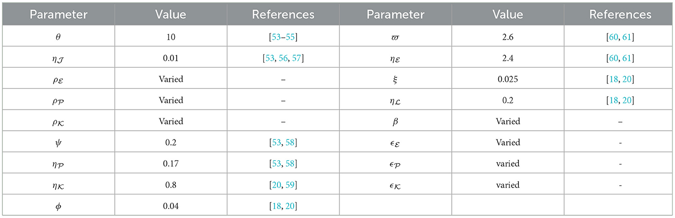
Table 1. Summary of model parameters and references.
I.S.1:
I.S.2:
I.S.3: .
Utilizing the infection rates ρZ for , the stability of steady states is governed by ℜ0(40), as defined in Equation (41). To scrutinize the impact of variations in these parameters, we explore two distinct scenarios:
Stability of O0(40). For the parameters , ϵ = 0.02, and β = 0.001, the computed value of ℜ0(40) = 0.503 is below 1. As illustrated in Figure 1, the trajectories originating I.S.1-I.S.3 approach the steady state O0(40) = (1000, 0, 0, 0, 0). This observation reinforces the assertion that O0(40) is being G.A.S, aligning with the outcome established in Theorem 2.1. Biologically speaking, this situation implies the complete eradication of the infection, signifying the successful elimination of the pathogen by the human body.
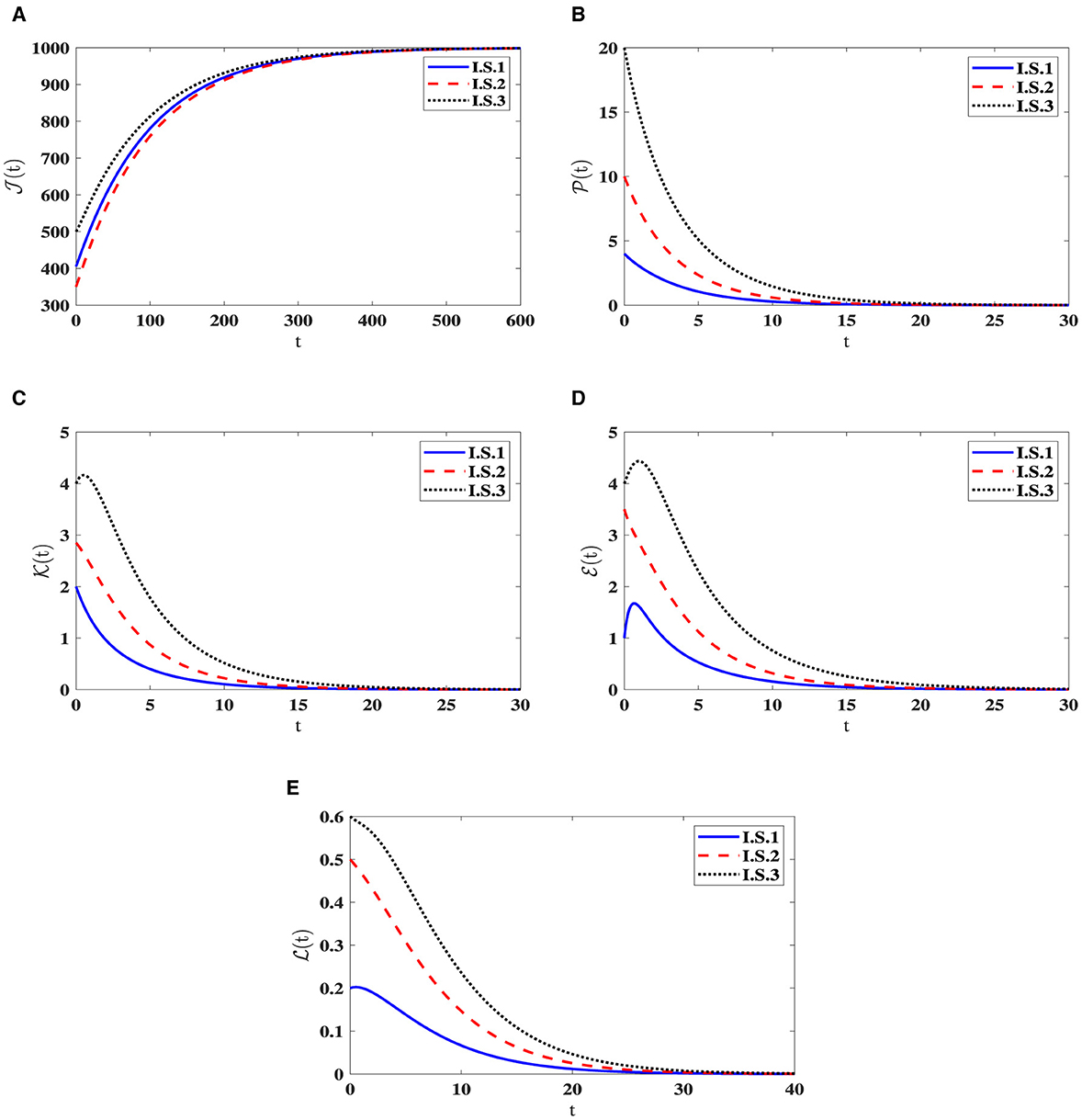
Figure 1. Solution patterns of the dynamical system (40) in the state of ℜ0(40) ≤ 1. (A) Healthy CD4+T cells. (B) Latently infected cells. (C) Actively infected cells. (D) HIV-1 particles. (E) CTLs.
Stability of O1(40). Choosing , ϵ = 0.02, and β = 0.001, yields ℜ0(40) = 2.804>1. Consequently, the steady state O1(40) exists when ℜ0(40) > 1, with specific values given by O1(40) = (408.467, 15.987, 3.903, 4.229, 0.479). In Figure 2, the numerical results align with the findings of Theorem 2.2, indicating the convergence of solutions for system (40) to O1(40) when ℜ0(40) > 1 across all I.S.1-I.S.3. From a biological standpoint, this situation implies the coexistence of both HIV-1 particles and CTLs within the host organism.
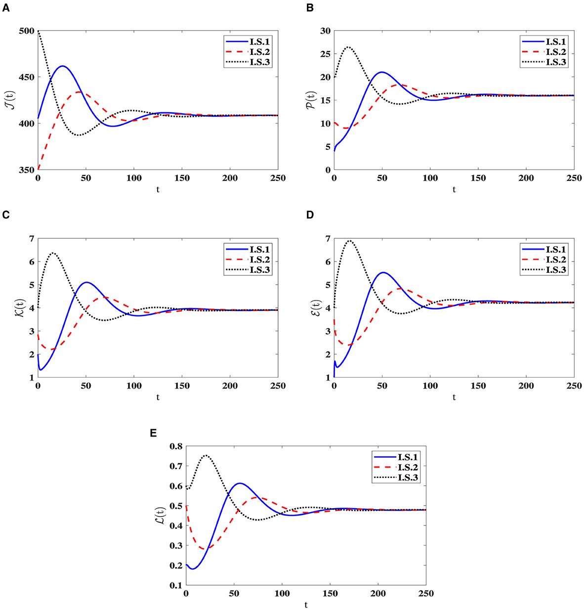
Figure 2. Solution patterns of the dynamical system (40) in the state of ℜ0(40) > 1. (A) Healthy CD4+T cells. (B) Latently infected cells. (C) Actively infected cells. (D) HIV-1 particles. (E) CTLs.
4.1.2 Impact of impaired CTL immunity
In this given context, we introduce fluctuations in the β value while maintaining specific values for , and ϵ = ϵZ = 0.02, where . We aim to explore how CTL immune impairment impacts the dynamics of the system (40), by obtaining numerical solutions with different β values as provided in Table 2. Under these circumstances, we employ the subsequent initial state:
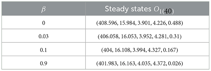
Table 2. Effect of the immune impairment parameter of CTLs on system (40).
I.S.4: .
As β increases, we notice a decline in the quantity of CTLs, as shown in Table 2. This decrease is accompanied by a greater quantity of infected cells, whether latent or active, along with a higher quantity of HIV-1 particles. Due to this, there is a reduction in the count of healthy cells. Notably, Figure 3 reveals that the stability criteria of the steady states remain unaffected by CTL immune impairment. This is a consequence of the fact that the parameter ℜ0(40) stays constant regardless of varying β values.
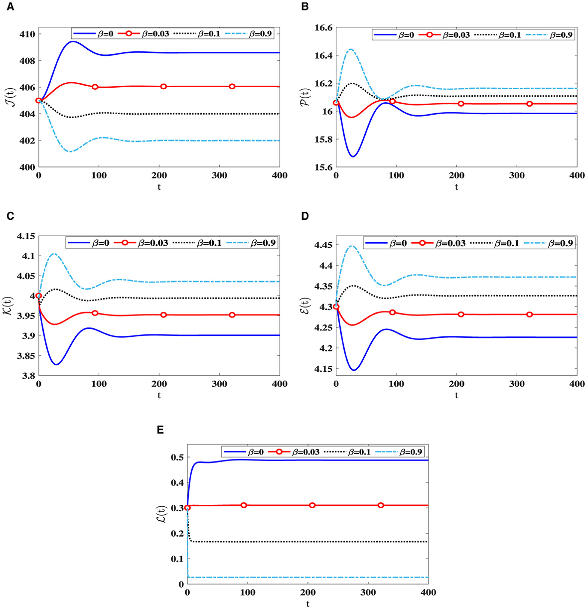
Figure 3. Solution patterns of the dynamical system (40) along different β values. (A) Healthy CD4+T cells. (B) Latently infected cells. (C) Actively infected cells. (D) HIV-1 particles. (E) CTLs.
4.1.3 The saturation infection rates effect on the system dynamics
In this instance, we fix specific values for , , , and β = 0.001. We numerically solve system (40) with various values of ϵ = ϵZ for , accompanied by the following initial state:
I.S.5: .
Upon examining the results in Table 3, a positive correlation is apparent between ϵ and healthy cells, meaning that when ϵ becomes higher, the concentration of healthy cells becomes higher too. In contrast, the counts of other compartments become lower. Notably, the parameter ℜ0(40) remains independent of ϵ. Consequently, Figure 4 illustrates that altering ϵ does not have an impact on the steady states' stability.
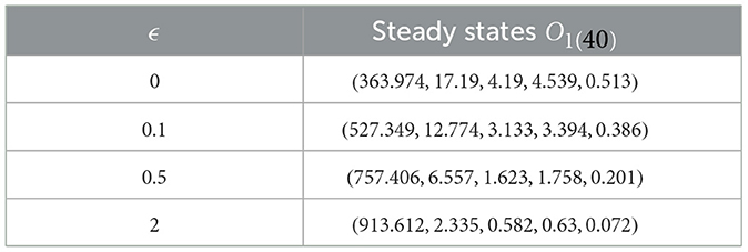
Table 3. Exploring system (40) dynamics under the influence of saturation infection rates.
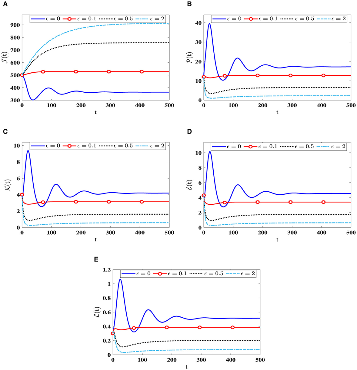
Figure 4. The influence of saturation infection rates on the solution patterns in system (40). (A) Healthy CD4+T cells. (B) Latently infected cells. (C) Actively infected cells. (D) HIV-1 particles. (E) CTLs.
4.2 Numerical simulation for model (23)
In the context of numerical analysis, we adopt the following specific form regarding the probability distribution functions πi(r), for i = 1, 2, 3:
where β*(.) is the Dirac delta function. When fi → ∞, we observe
Furthermore, we obtain
Additionally, we will select the Holling type-II incidence rates of infection as follows:
Here, the positive constants ρZ for denote the infection rate constants, while ϑ > 0 represents the Holling infection rate constant. Consequently, Based on the aforementioned reasoning, system (23) was modified into a system with a discrete time delay, as illustrated below:
The functions for are evidently continuously differentiable. Additionally, for each , these functions satisfy the conditions: and for all and Z > 0. Thus, the fulfillment of Condition C1 is evident. Furthermore, we observe
where . This can be expressed by stating that Condition C2 is valid. It is obvious that
Furthermore
which confirms that Condition C3 is also met. Moreover, we have
Hence, the verification of Condition C4 is straightforward. Additionally, it is evident that for . Consequently, Condition C5 is satisfied. Moreover, we have:
and
for all . Hence, Condition C6 is fulfilled as well. With the fulfillment of Conditions C1 –C6, the global stability results stated in Theorems 3.1 and 3.2 persist. Accordingly, the determination of the basic reproduction ratio for system (42) is outlined below:
where
4.2.1 The stability implications of time delays on steady states
To assess how time delay parameters affect the solutions of system (42), we maintain constant values for parameters , , , β = 0.001, b1 = 0.1, b2 = 0.2, b3 = 0.3, and set ϑ = 0.0001. Furthermore, you can refer to Table 1 for the values of the other parameters. Next, we examine how the dynamics are affected by experimenting with different variations of the delay parameters ri, where i takes values from 1 to 3. The stability of steady states is highly sensitive to changes in the parameters ri due to the dependence of on them [as indicated in Equation (43)]. Let's delve into the following choices for the delay parameters:
D.P.1: r1 = 0.003, r2 = 0.001, r3 = 0.002.
D.P.2: r1 = 0.01, r2 = 0.02, r3 = 0.03.
D.P.3: r1 = 0.8, r2 = 0.6, r3 = 0.7.
D.P.4: r1 = 1.189, r2 = 1.5, r3 = 2.5.
D.P.5: r1 = 3, r2 = 4, r3 = 5.
D.P.6: r1 = 5, r2 = 6, r3 = 7. We address the initial state for solving system (42) as follows:
I.S.6: , v∈[−r, 0], r = max{r1, r2, r3}. Table 4 displays the values of corresponding to different ri values, where i = 1, 2, 3. Significantly reducing is noteworthy when the ri parameters increase. Figure 5 visually depicts the numerical solutions derived from the system, emphasizing the significant impact of the included time-delays. Specifically, a positive correlation exists between ri and the count of healthy cells, indicating that their values increase simultaneously, while a decrease is observed in the counts of other compartments. This suggests the potential creation of a new category of medication aimed at extending delay times and ultimately mitigating HIV-1 multiplication.
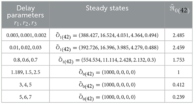
Table 4. Analyzing the influence of delay parameters, ri, on System (42).
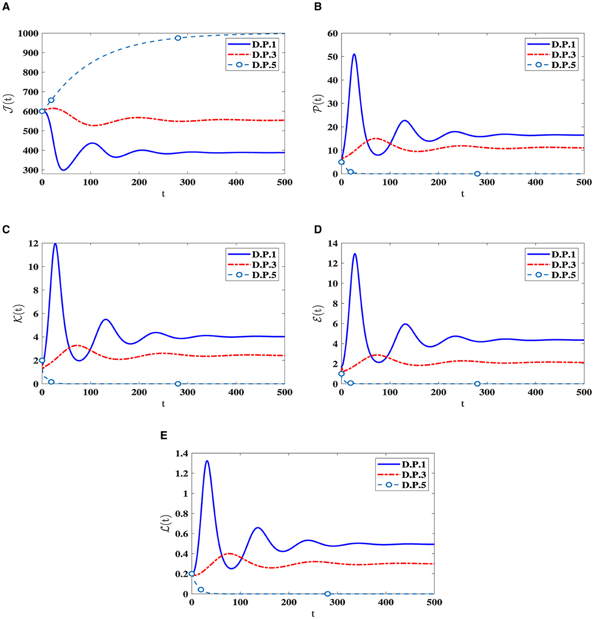
Figure 5. The influence of ri on the solution patterns in system (42). (A) Healthy CD4+T cells. (B) Latently infected cells. (C) Actively infected cells. (D) HIV-1 particles. (E) CTLs.
4.2.2 The Holling type-II infection rates effect on the system dynamics
In this scenario, we set , , , b1 = 0.1, b2 = 0.2, b3 = 0.3, β = 0.001, and ri = 0.002 for i = 1, 2, 3. We consider different values of ϑ and numerically solve system (42) with the initial state I.S.6 to analyze the impact of Holling infection rates on the dynamics of the system (42). Analyzing Table 5 reveals a correlation wherein an augmentation in ϑ leads to an increase in the count of healthy cells, while there is a reduction in the counts of other compartments. Clearly, the parameter depends on ϑ. Therefore, Figure 6 confirms that the Holling infection alters the stability properties of steady states. Furthermore, we derive the subsequent observations:
1. Õ1(42) is being G.A.S under the condition 0 < ϑ < 0.0017336.
2. Õ0(42) is being G.A.S under the condition ϑ≥0.0017336.
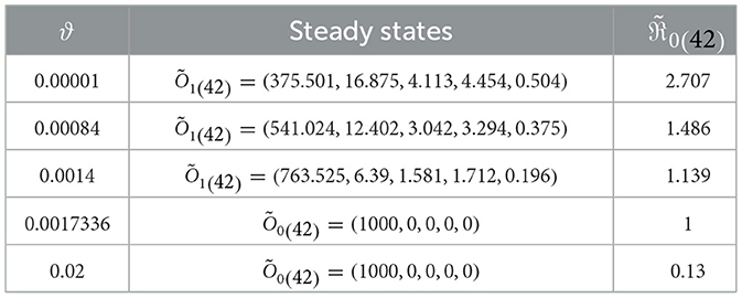
Table 5. The dynamics of system (42) affected by Holling infection rates.
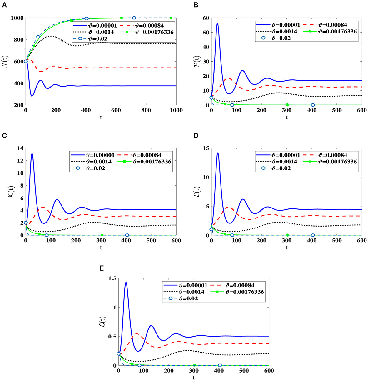
Figure 6. The influence of Holling infection rates on the solution patterns in system (42). (A) Healthy CD4+T cells. (B) Latently infected cells. (C) Actively infected cells. (D) HIV-1 particles. (E) CTLs.
4.3 Analysis of parameter sensitivity
4.3.1 Investigating the sensitivity of parameters for model (40)
The principal goal of analyzing parameter sensitivity is to determine the variable that has the most substantial impact on ℜ0, which should be the focus of control strategies. To achieve this, we will employ direct differentiation, a method that calculates sensitivity indices by considering changes in variables based on parameters. We can define the normalized forward sensitivity index of ℜ0, which depends on the differentiability with respect to a parameter ϱ, as follows:
For each parameter belonging to ℜ0(40), we utilized Equation (44) to compute the sensitivity index values. For this purpose, we considered the parameters specified in Table 1, while also incorporating supplementary values for , , and . Sensitivity index values for ℜ0(40) are showcased in Table 6 and Figure 7, revealing positive index values for θ, , , , ϖ, and ψ. In this context, higher values of these parameters correspond to a higher prevalence of HIV-1 infection within this population. In contrast, the remaining indices show negativity, implying that an increase in , , , and corresponds to a reduction in the ℜ0(40) value. Notably, the parameters θ, , and ϖ emerge as the pivotal factors in terms of sensitivity, whereas , , and ψ are considered less critical. Interestingly, the parameter ξ, representing CTLs responsiveness, demonstrates no impact on ℜ0(40).

Table 6. Examining sensitivity in parameters regarding ℜ0(40).
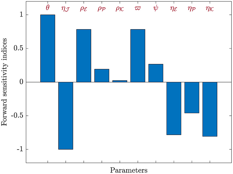
Figure 7. Analyzing sensitivity of parameters for ℜ0(40) in model (40).
4.3.2 Investigating the sensitivity of parameters for model (42)
Here, Equation (44) will be applied to calculate sensitivity indices concerning , considering each parameter contributing to the basic reproduction ratio. The calculations were performed with the parameters specified in Table 1, supplemented by the inclusion of the additional parameters: , , , b1 = 0.1, b2 = 0.2, b3 = 0.3, r1 = 0.8, r2 = 0.6, r3 = 0.7, and ϑ = 0.0001. The sensitivity index values for are presented in Table 7, and Figure 8 provides a graphical representation. Positive indices for θ, , , , ϖ, and ψ suggest that an increase in these values will elevate the prevalence of HIV-1 disease. Conversely, negative indices, including , , , , b1, b2, b3, r1, r2, r3, and ϑ, indicate that an increase in these values will lower the parameter . Notably, θ, , and ϖ emerge as the most influential parameters, while , , and ψ are considered less critical. Furthermore, the parameter representing CTLs responsiveness, ξ, demonstrates no discernible effect on .
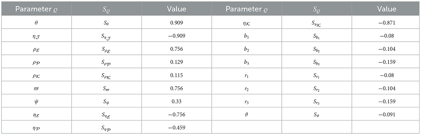
Table 7. Examining sensitivity in parameters regarding .
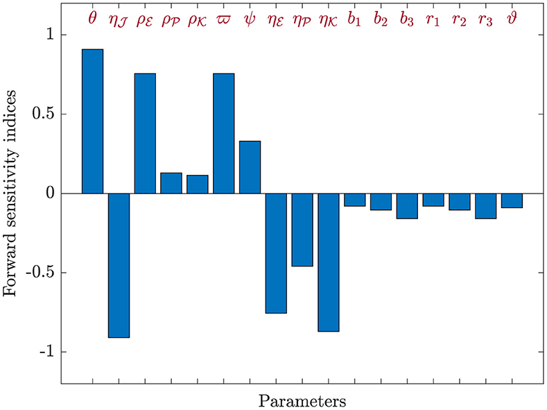
Figure 8. Analyzing sensitivity of parameters for in model (42).
5 Discussion
To emphasize the importance of integrating L-CTC spread into our investigated models, we analyze model (3) in the context of various antiviral interventions, outlined as follows:
The parameter 0 ≤ ς1 ≤ 1 represents the effectiveness of antiviral therapy in inhibiting VTC transmission, while 0 ≤ ς2, ς3 ≤ 1 denote the therapeutic efficacies in blocking L-CTC and A-CTC transmissions, respectively [62].
For system (45), the following establishes the basic reproduction ratio:
Assuming ς to be equal to ς1, ς2, and ς3, we obtain:
Currently, we compute the drug efficacy, ς, which results in and stabilizes O0 in system (45) as follows:
Neglecting the spread of L-CTC in model (45) yields
and the definition of the basic reproduction ratio of model (47) will be
We identify the drug efficacy, denoted as ς, that ensures , thereby stabilizing the steady state O0 of system (47). The condition is expressed as:
It is evident that . Interestingly, comparing Equations (46, 48) reveal that is always smaller than . Therefore, applying drugs with efficacy ς in case of will guarantee that , ensuring the global asymptotic stability of O0 in the system (47). However, , indicating the instability of O0 in system (45). As a result, drug therapies are designed without considering the spread of L-CTC may be inaccurate or insufficient for achieving viral eradication from the body. Therefore, compared to the model given in Alofi and Azoz [24] and Zhang and Xu [25], our suggested models are more pertinent in explaining HIV-1 infections.
6 Conclusion
This work formulates two HIV-1 dynamics models with CTL immune impairment. These models comprise five compartments: healthy CD4+T cells, latently infected cells, actively infected cells, free HIV-1 and CTLs. To enhance realism, we introduced a scenario in which healthy cells acquire susceptibility to infection upon exposure to infectious compartments (HIV-1 particles, latently infected cells and actively infected cells). The second model takes the first model a step further by incorporating multiple distributed-time delays. Both models incorporate general functions to represent the incidence rates. Notably, the solutions produced by these models display properties of nonnegativity and boundedness. Within this framework, we identified two crucial steady states: the virus-free steady state, O0 (Õ0), and the virus-persistence steady state, O1 (Õ1). We calculated the basic reproduction ratios, referred to as ℜ0 (), which are essential for determining whether the steady states mentioned earlier exist and remain stable over time. It is noteworthy that ℜ0 () consists of three separate components, representing the contributions from VTC, L-CTC, and A-CTC. The Lyapunov function technique and L.I.P. are employed to comprehend the system's behavior over time by studying the global asymptotic stability of the steady states. Two key findings emerged from our investigation: firstly, the virus-free steady state O0 (Õ0) is being G.A.S whenever ℜ0 < 1 (), ultimately leading to the disappearance of the infection. In contrast, the steady state O0 (Õ0) loses its stability and the virus-persistence steady state O1 (Õ1) is being G.A.S whenever ℜ0 > 1 (), indicating a long-term infection. For experimental verification of our theoretical derivations, we employed numerical simulations, which yielded results consistent with our analytical solutions. Our exploration encompassed the influence of CTL immune impairment, time delays, and L-CTC on HIV-1 dynamics, revealing reduced immune function as a key factor contributing significantly to disease progression. Moreover, time delays significantly reduced the basic reproduction ratio (), leading to suppressed HIV-1 reproduction. Therefore, eliminating HIV-1 requires prioritizing strategies that keep below 1. Our study also highlights the critical role of L-CTC spread in HIV-1 dynamics. Additionally, a sensitivity analysis revealed key factors influencing the system's behavior, deepening our understanding of HIV-1 dynamics.
We are optimistic that the strategy outlined in our article may be improved upon. The modeling of the in-host dynamics with an emphasis on the immune system vs invading particles would be an intriguing viewpoint. Recently, active-particle approaches have been utilized to describe the immunological rivalry in detail at the cellular level, allowing for the modeling of epidemics (see [63]).
It seems like an interesting avenue to investigate the memory impact on the dynamics of our model with fractional differential equations (FDEs) [64–66]. Non-local and memory-dependent effects, which are frequently essential in virological systems, can be captured by FDEs. In our proposed modeled we assumed that the production rate of healthy CD4+T cells is constant. Nonetheless, HIV-1 infection possesses the capability to infect and disrupt the thymus's supply of these cells. As a result, rather than being constant, the thymus's supply of new cells has been seen to be changeable [55, 67]. These topics are left for later research.
Data availability statement
The original contributions presented in the study are included in the article/supplementary material, further inquiries can be directed to the corresponding author.
Author contributions
AE: Conceptualization, Formal analysis, Methodology, Writing – original draft, Writing – review & editing. NA: Conceptualization, Formal analysis, Investigation, Methodology, Writing – original draft, Writing – review & editing. RH: Formal analysis, Investigation, Methodology, Writing – original draft, Writing – review & editing.
Funding
The author(s) declare that no financial support was received for the research, authorship, and/or publication of this article.
Conflict of interest
The authors declare that the research was conducted in the absence of any commercial or financial relationships that could be construed as a potential conflict of interest.
Publisher's note
All claims expressed in this article are solely those of the authors and do not necessarily represent those of their affiliated organizations, or those of the publisher, the editors and the reviewers. Any product that may be evaluated in this article, or claim that may be made by its manufacturer, is not guaranteed or endorsed by the publisher.
References
1. Nowak MA, May RM. Virus Dynamics. New York, NY: Oxford University Press (2000). doi: 10.1093/oso/9780198504184.001.0001
2. Nowak MA, Bangham CRM. Population dynamics of immune responses to persistent viruses. Science. (1996) 272:74–9. doi: 10.1126/science.272.5258.74
3. Jan R, Khan A, Boulaaras S, Zubair SA. Dynamical behaviour and chaotic phenomena of HIV infection through fractional calculus. Discrete Dyn Nat Soc. (2022) 2022:5937420. doi: 10.1155/2022/5937420
4. Jan A, Srivastava HM, Khan A, Mohammed PO, Jan R, Hamed YS, et al. In vivo HIV dynamics, modeling the interaction of HIV and immune system via non-integer derivatives. Fractal Fract. (2023) 7:361. doi: 10.3390/fractalfract7050361
5. Jan R, Boulaaras S, Shah SAA. Fractional-calculus analysis of human immunodeficiency virus and CD4+ T-cells with control interventions. Commun Theor Phys. (2022) 74:105001. doi: 10.1088/1572-9494/ac7e2b
6. Jolly C, Sattentau Q. Retroviral spread by induction of virological synapses. Traffic. (2004) 5:643–50. doi: 10.1111/j.1600-0854.2004.00209.x
7. Komarova NL, Wodarz D. Virus dynamics in the presence of synaptic transmission. Math Biosci. (2013) 242:161–71. doi: 10.1016/j.mbs.2013.01.003
8. Sigal A, Kim JT, Balazs AB, Dekel E, Mayo A, Milo R, et al. Cell-to-cell spread of HIV permits ongoing replication despite antiretroviral therapy. Nature. (2011) 477:95–8. doi: 10.1038/nature10347
9. Gao Y, Wang J. Threshold dynamics of a delayed nonlocal reaction-diffusion HIV infection model with both cell-free and cell-to-cell transmissions. J Math Anal Appl. (2020) 488:124047. doi: 10.1016/j.jmaa.2020.124047
10. Graw F, Perelson AS. Modeling viral spread. Ann Rev Viro. (2016) 3:555–72. doi: 10.1146/annurev-virology-110615-042249
11. Guo T, Qiu Z. The effects of CTL immune response on HIV infection model with potent therapy, latently infected cells and cell-to-cell viral transmission. Math Biosci Eng. (2019) 16:6822–41. doi: 10.3934/mbe.2019341
12. Wang J, Guo M, Liu X, Zhao Z. Threshold dynamics of HIV-1 virus model with cell-to-cell transmission, cell-mediated immune responses and distributed delay. Appl Math Comput. (2016) 291:149–61. doi: 10.1016/j.amc.2016.06.032
13. Yang Y, Zhang T, Xu Y, Zhou J. A delayed virus infection model with cell-to-cell transmission and CTL immune response. Int J Bifurcat Chaos. (2017) 27:1750150. doi: 10.1142/S0218127417501504
14. Cervantes-Perez AG, Avila-Vales E. Dynamical analysis of multipathways and multidelays of general virus dynamics model. Int J Bifurcat Chaos. (2019) 29:1950031–30. doi: 10.1142/S0218127419500317
15. Elaiw AM, AlShamrani NH. Global stability of a delayed adaptive immunity viral infection with two routes of infection and multi-stages of infected cells. Commun Nonlinear Sci Numer Simul. (2020) 86:105259. doi: 10.1016/j.cnsns.2020.105259
16. Regoes R, Wodarz D, Nowak MA. Virus dynamics: the effect to target cell limitation and immune responses on virus evolution. J Theor Biol. (1998) 191:451–62. doi: 10.1006/jtbi.1997.0617
17. Hu Z, Zhang J, Wang H, Ma W, Liao F. Dynamics analysis of a delayed viral infection model with logistic growth and immune impairment. Appl Math Model. (2014) 38:524–34. doi: 10.1016/j.apm.2013.06.041
18. Krishnapriya P, Pitchaimani M. Modeling and bifurcation analysis of a viral infection with time delay and immune impairment. Jpn J Ind Appl Math. (2017) 34:99–139. doi: 10.1007/s13160-017-0240-5
19. Eric AV, Noe CC, Gerardo GA. Analysis of a viral infection model with immune impairment, intracellular delay and general non-linear incidence rate. Chaos Solitons Fractals. (2014) 69:1–9. doi: 10.1016/j.chaos.2014.08.009
20. Wang S, Song X, Ge Z. Dynamics analysis of a delayed viral infection model with immune impairment. Appl Math Model. (2011) 35:4877–85. doi: 10.1016/j.apm.2011.03.043
21. Krishnapriya P, Pitchaimani M. Analysis of time delay in viral infection model with immune impairment. J Appl Math Comput. (2017) 55:421–53. doi: 10.1007/s12190-016-1044-5
22. Wang ZP, Liu XN. A chronic viral infection model with immune impairment. J Theor Biol. (2007) 249:532–42. doi: 10.1016/j.jtbi.2007.08.017
23. Elaiw AM, Raezah A, Alofi BS. Dynamics of delayed pathogen infection models with pathogenic and cellular infections and immune impairment. AIP Adv. (2018) 8:025323. doi: 10.1063/1.5023752
24. Alofi BS, Azoz SA. Stability of general pathogen dynamic models with two types of infectious transmission with immune impairment. AIMS Mathem. (2020) 6:114–40. doi: 10.3934/math.2021009
25. Zhang L, Xu R. Dynamics analysis of an HIV infection modelwith latent reservoir, delayed CTL immune response and immune impairment. Nonlinear Anal Model Control. (2023) 28:1–19. doi: 10.15388/namc.2023.28.29615
26. Xu R, Song C. Dynamics of an HIV infection model with virus diffusion and latently infected cell activation. Nonlinear Anal Real World Appl. (2022) 67:103618. doi: 10.1016/j.nonrwa.2022.103618
27. Nath BJ, Sadri K, Sarmah HK, Hosseini K. An optimal combination of antiretroviral treatment and immunotherapy for controlling HIV infection. Math Comput Simul. (2024) 217:226–43. doi: 10.1016/j.matcom.2023.10.012
28. Agosto L, Herring M, Mothes W, Henderson A. HIV-1-infected CD4+ T cells facilitate latent infection of resting CD4+ T cells through cell-cell contact. Cell. (2018) 24:2088–100. doi: 10.1016/j.celrep.2018.07.079
29. Wang W, Wang X, Guo K, Ma W. Global analysis of a diffusive viral model with cell-to-cell infection and incubation period. Math Methods Appl Sci. (2020) 43:5963–78. doi: 10.1002/mma.6339
30. Hattaf K, Dutta H. Modeling the dynamics of viral infections in presence of latently infected cells. Chaos Solitons Fractals. (2020) 136:109916. doi: 10.1016/j.chaos.2020.109916
31. Elaiw AM, AlShamrani NH. Stability of a general CTL-mediated immunity HIV infection model with silent infected cell-to-cell spread. Adv Diff Equ. (2020) 2020:355. doi: 10.1186/s13662-020-02818-3
32. Li J, Wang X, Chen Y. Analysis of an age-structured HIV infection model with cell-to-cell transmission. Eur Phys J Plus. (2024) 139:78. doi: 10.1140/epjp/s13360-024-04873-1
33. Bai N, Xu R. Mathematical analysis of an HIV model with latent reservoir, delayed CTL immune response and immune impairment. Math Biosc Eng. (2021) 18:1689–707. doi: 10.3934/mbe.2021087
34. AlShamrani NH, Halawani RH, Shammakh W, Elaiw AM. Global properties of HIV-1 dynamics models with CTL immune impairment and latent cell-to-cell spread. Mathematics. (2023) 11:3743. doi: 10.3390/math11173743
35. AlShamrani NH, Halawani RH, Elaiw AM. Effect of impaired B-cell and CTL functions on HIV-1 dynamics. Mathematics. (2023) 11:4385. doi: 10.3390/math11204385
36. Ma Y, Yu X. The effect of environmental noise on threshold dynamics for a stochastic viral infection model with two modes of transmission and immune impairment. Chaos Solitons Fractals. (2020) 134:109699. doi: 10.1016/j.chaos.2020.109699
37. Yang Y, Xu R. Mathematical analysis of a delayed HIV infection model with saturated CTL immune response and immune impairment. J Appl Math Comput. (2022) 68:2365–80. doi: 10.1007/s12190-021-01621-x
38. Yaagoub Z, Sadki M, Allali K. A generalized fractional hepatitis B virus infection modelwith both cell-to-cell and virus-to-cell transmissions. Nonlinear Dyn. (2024). doi: 10.21203/rs.3.rs-3958680/v1
39. Elaiw AM, AlShamrani NH. Global stability of humoral immunity virus dynamics models with nonlinear infection rate and removal. Nonlinear Anal: Real World Appl. (2015) 26:161–90. doi: 10.1016/j.nonrwa.2015.05.007
40. Shu H, Chen Y, Wang L. Impacts of the cell-free and cell-to-cell infection modes on viral dynamics. J Dynam Differential Equations. (2018) 30:1817–36. doi: 10.1007/s10884-017-9622-2
41. Smith HL, Waltman P. The Theory of the Chemostat: Dynamics of Microbial Competition. Cambridge: Cambridge University Press (1995). doi: 10.1017/CBO9780511530043
42. van den Driessche P, Watmough J. Reproduction numbers and sub-threshold endemic equilibria for compartmental models of disease transmission. Math Biosci. (2002) 180:29–48. doi: 10.1016/S0025-5564(02)00108-6
43. Korobeinikov A. Global properties of basic virus dynamics models. Bull Math Biol. (2004) 66:879–83. doi: 10.1016/j.bulm.2004.02.001
44. Hale JK, Lunel SMV. Introduction to Functional Differential Equations. New York, NY: Springer-Verlag (1993). doi: 10.1007/978-1-4612-4342-7
46. Perelson A, Neumann A, Markowitz M, Leonard J, Ho D. HIV-1 dynamics in vivo: virion clearance rate, infected cell life-span, and viral generation time. Science. (1996) 271:1582–6. doi: 10.1126/science.271.5255.1582
47. Culshaw RV, Ruan S, Webb G. A mathematical model of cell-to-cell spread of HIV-1 that includes a time delay. J Math Biol. (2003) 46:425–44. doi: 10.1007/s00285-002-0191-5
48. Lai X, Zou X. Modelling HIV-1 virus dynamics with both virus-to-cell infection and cell-to-cell transmission. SIAM J Appl Math. (2014) 74:898–917. doi: 10.1137/130930145
49. Elaiw AM, Raezah AA. Stability of general virus dynamics models with both cellular and viral infections and delays. Math Methods Appl Sci. (2017) 40:5863–80. doi: 10.1002/mma.4436
50. Adak D, Bairagi N. Analysis and computation of multi-pathways and multi-delays HIV-1 infection model. Appl Math Model. (2018) 54:517–36. doi: 10.1016/j.apm.2017.09.051
51. Yang Y, Zou L, Ruan S. Global dynamics of a delayed within-host viral infection model with both virus-to-cell and cell-to-cell transmissions. Math Biosci. (2015) 270:183–91. doi: 10.1016/j.mbs.2015.05.001
52. Kuang Y. Delay Differential Equations with Applications in Population Dynamics. San Diego: Academic Press (1993).
53. Sahani SK, Yashi. Effects of eclipse phase and delay on the dynamics of HIV infection. J Biol Syst. (2018) 26:421–54. doi: 10.1142/S0218339018500195
54. Li F, Ma W. Dynamics analysis of an HTLV-1 infection model with mitotic division of actively infected cells and delayed CTL immune response. Math Methods Appl Sci. (2018) 41:3000–17. doi: 10.1002/mma.4797
55. Perelson AS, Kirschner DE, de Boer R. Dynamics of HIV infection of CD4+ T cells. Math Biosci. (1993) 114:81–125. doi: 10.1016/0025-5564(93)90043-A
56. Callaway DS, Perelson AS. HIV-1 infection and low steady state viral loads. Bull Math Biol. (2002) 64:29–64. doi: 10.1006/bulm.2001.0266
57. Mohri H, Bonhoeffer S, Monard S, Perelson AS, Ho DD. Rapid turnover of T lymphocytes in SIV-infected rhesus macaques. Science. (1998) 279:1223–7. doi: 10.1126/science.279.5354.1223
58. Wang Y, Liu J, Liu L. Viral dynamics of an HIV model with latent infection incorporating antiretroviral therapy. Adv Differ Equ. (2016) 2016:225. doi: 10.1186/s13662-016-0952-x
59. Yan C, Wang W. Modeling HIV dynamics under combination therapy with inducers and antibodies. Bull Math Biol. (2019) 81:2625–48. doi: 10.1007/s11538-019-00621-0
60. Allali K, Danane J, Kuang Y. Global analysis for an HIV infection model with CTL immune response and infected cells in eclipse phase. Appl Sci. (2017) 7:861. doi: 10.3390/app7080861
61. Sun Q, Min L, Kuang Y. Global stability of infection-free state and endemic infection state of a modified human immunodeficiency virus infection model. IET Syst Biol. (2015) 9:95–103. doi: 10.1049/iet-syb.2014.0046
62. Wang X, Rong L. HIV low viral load persistence under treatment: insights from a model of cell-to-cell viral transmission. Appl Math Lett. (2019) 94:44–51. doi: 10.1016/j.aml.2019.02.019
63. Burini D, Knopoff D. Epidemics and society-a multiscale vision from the small world to the globally interconnected world. Math Models Methods Appl Sci. (2024) 34:1564–96. doi: 10.1142/S0218202524500295
64. Boulaaras S, Rehman ZU, Abdullah FA, Jan R, Abdullah M, Jan A, et al. Coronavirus dynamics, infections and preventive interventions using fractional-calculus analysis. AIMS Math. (2023) 8:8680–701. doi: 10.3934/math.2023436
65. Tang TQ, Shah Z, Jan R, Deebani W, Shutaywi M. A robust study to conceptualize the interactions of CD4+ T-cells and human immunodeficiency virus via fractional-calculus. Phys Scr. (2021) 96:125231. doi: 10.1088/1402-4896/ac2d7b
66. Hattaf K. A new mixed fractional derivative with applications in computational biology. Computation. (2024) 12:7. doi: 10.3390/computation12010007
Keywords: HIV-1, immune impairment, global stability, delays, Lyapunov stability, sensitivity analysis
Citation: AlShamrani NH, Halawani RH and Elaiw AM (2024) Stability of generalized models for HIV-1 dynamics with impaired CTL immunity and three pathways of infection. Front. Appl. Math. Stat. 10:1412357. doi: 10.3389/fams.2024.1412357
Received: 04 April 2024; Accepted: 15 July 2024;
Published: 14 August 2024.
Edited by:
Fahad Al Basir, Asansol Girls' College, IndiaReviewed by:
Rashid Jan, University of Swabi, PakistanZakaria Yaagoub, University of Hassan II Casablanca, Morocco
Nicola Bellomo, Polytechnic University of Turin, Italy
Copyright © 2024 AlShamrani, Halawani and Elaiw. This is an open-access article distributed under the terms of the Creative Commons Attribution License (CC BY). The use, distribution or reproduction in other forums is permitted, provided the original author(s) and the copyright owner(s) are credited and that the original publication in this journal is cited, in accordance with accepted academic practice. No use, distribution or reproduction is permitted which does not comply with these terms.
*Correspondence: Noura H. AlShamrani, bmhhbHNoYW1yYW5pQHVqLmVkdS5zYQ==