A robust, exponentially fitted higher-order numerical method for a two-parameter singularly perturbed boundary value problem

This study constructs a robust higher-order fitted operator finite difference method for a two-parameter singularly perturbed boundary value problem. The derivatives in the governing ordinary differential equation are substituted by second-order central finite difference approximations, after which the fitting parameter is introduced and determined. The resulting system of linear equations may then be solved using the Thomas method. The stability, consistency, and convergence of the current method have been thoroughly validated. To enhance accuracy and achieve a higher-order numerical solution, a post-processing technique was employed to upgrade the method from second-order to fourth-order convergence. Finally, three test examples were used to confirm the method's appropriateness. The numerical results demonstrate that the proposed technique is stable, consistent, and produces a higher-order numerical solution than the existing ones in the literature.

1 Introduction

Singularly perturbed differential equations involve the highest-order derivative term being multiplied by a small perturbation parameter, ε. In the context of singularly perturbed problems, differential equations with two small parameters affecting the diffusion and convection terms are intriguing areas of research. The main purpose of this study is to obtain a robust higher-order numerical method to solve a two-parameter singularly perturbed boundary value problem. Find Υ such that

$\begin{array}{ll}{\Pi }_{\epsilon ,\mu }{\rm Y}\left(\theta \right)\equiv -\epsilon {{\rm Y}}^{\prime \prime }\left(\theta \right)+\mu a\left(\theta \right){{\rm Y}}^{\prime }\left(\theta \right)+b\left(\theta \right){\rm Y}\left(\theta \right)=f\left(\theta \right),\theta \in \Omega =\left(0,1\right),& (1)\end{array}$

subject to the boundary conditions

$\begin{array}{ll}{\rm Y}\left(0\right)={\gamma }_0,{\rm Y}\left(1\right)={\gamma }_1,& (2)\end{array}$

where ε(0 < ε ≪ 1) and μ(0 < μ ≪ 1) are the small parameters that make the differential equation singularly perturbed. Let us assume the functions a(θ), b(θ) and f(θ) are sufficiently smooth and bounded to ensure the existence of a unique solution. Assume that there exist constants α, β and ζ independent of ε and μ such that for any θ = [0, 1] the conditions,

$a\left(\theta \right)\ge \alpha >0,b\left(\theta \right)\ge \beta >0,b\left(\theta \right)-\frac{1}{2}\mu a^{\prime }\left(\theta \right)\ge \zeta >0,$

hold for some constant α, β and ζ. Assume $\delta \approx \underset{x\in \bar{\Omega }}{min}\frac{b\left(\theta \right)}{a\left(\theta \right)}$. When μ = 1, Equation 1 is reduced to the singularly perturbed convection-diffusion boundary value problem. When μ = 0, Equation 1 reduces to a well-known singularly perturbed reaction-diffusion boundary value problem. The mathematical model for the kind of Equation 1 often arises in chemical reactor theory [1], transport phenomena in chemistry and biology [2], and lubrication theory [3]. The nature of the two-parameter problem was asymptotically examined by O'Malley [4], where the ratio of μ to ε has significant role in the solution. For this problem, two boundary layers occur at θ = 0 and θ = 1. Because of the presence of these layers, some standard numerical methods in Lodhi et al. [5], Kambampati et al. [6], Pandit and Kumar [7], Khandelwal and Khan [8] are applied to a uniform mesh, which provides an oscillatory numerical solution. Consequently, considerable attention has been devoted to using non-uniform meshes to solve two-parameter singularly perturbed boundary value problems, as discussed in works by O'Riordan and Pickett [9], Roos and Uzelac [10], Kadalbajoo and Yadaw [11], Kadalbajoo and Jha [12], Brdar and Zarin [13], Luo et al. [14], Brdar and Zarin [15, 16], Padmaja et al. [17], Andisso and Duressa [18], Linß and Roos [19], Cheng [20], Zhang and Lv [21], Valarmathi and Ramanujam [22], Patidar [23] to solve two-parameter singularly perturbed boundary value problems. The majority of the previously developed methods to solve the problem at hand are less accurate and of lower order. Inspired by this, the goal of this study is to offer a high order and more accurate fitted operator method with the help of post-processing technique to solve the considered problem. Because of the presence of boundary layer in the solution of Equation 1, devising a higher-order convergent numerical method is a big challenge. In this study, we apply the well-known post-processing technique of Richardson extrapolation method to obtain fourth order uniformly convergent numerical solution of Equation 1. The present approach yields a more accurate solution in terms of maximum absolute errors than previous approaches found in the literature.

Some robust numerical methods for one-parameter and two-parameter singularly perturbed problems in studies by Hassen and Duressa [24], Mohye et al. [25], Tesfaye et al. [26], Cheru et al. [27], Daba et al. [28], Gupta et al. [29], singularly perturbed turning point problem in Gupta et al. [30], time-fractional singularly perturbed convection-diffusion problem [31], singularly perturbed problems with spatio-time delays the study by Ejere et al. [32] and singularly perturbed problems Burger-Huxley problem in the study by Daba and Duressa [33] and Derzie et al. [34]. Some methods are employed studies by Li et al. [35], El Ahmadi et al. [36], Nachaoui [37], Mardanov et al. [38] to solve different types of differential equations.

The remaining part of the article is arranged as follows: In Section 2, we have provided a brief description of the present method for the numerical solution of Equations 1, 2. The convergence analysis of the method is presented in Section 3. Section 4 presents the numerical results, and comparisons are made with other existing methods. Finally, the conclusion is provided at the end of the article in Section 5.

2 The continuous problem

In this section, we provide a priori bounds for the solution and its corresponding derivatives. The governing problem in Equations 1, 2 exhibits twin boundary layers with different layer widths depending on the relation between the values of ε and μ. If αμ² ≤ δε, then the reduced problem corresponding to Equations 1, 2 is given by

$b\left(\theta \right){\rm Y}\left(\theta \right)=f\left(\theta \right).$

Thus, the boundary layers are expected near θ = 0 and θ = 1, with a width of $O\left(\sqrt{\epsilon }\right)$ if Υ₀(0) ≠ γ₀ and Υ₀(1) ≠ γ₁. If αμ² ≥ δε, then the reduced problem corresponding to Equations 1, 2 is given by

$\begin{array}{r}\mu a\left(\theta \right){{\rm Y}}_{\mu }^{\prime }\left(\theta \right)+b\left(\theta \right){{\rm Y}}_{\mu }\left(\theta \right)=f\left(\theta \right),\\ {{\rm Y}}_{\mu }\left(0\right)={\gamma }_0.\end{array}$

Thus, the boundary layer of width O(ε/μ) is expected in the right neighborhood of θ = 0 if Υ_μ(0) ≠ γ₀ and the boundary layer of width O(μ) is expected in the left neighborhood of θ = 1 if Υ_μ(1) ≠ γ₁. The assumptions given for Equations 1, 2 ensure that the differential operator Π_{ε, μ} satisfies the following maximum principle.

Lemma 1. Let ϖ(θ) be a smooth function such that ϖ(0) ≥ 0 and ϖ(1) ≥ 0. If Π_ε,μ ϖ(θ) ≥ 0, for θ ∈ Ω, then ϖ(θ) ≥ 0, for $\theta \in \bar{\Omega }$.

Proof. Assume θ^* be such that $\varpi \left({\theta }^{*}\right)=\underset{\theta \in \bar{\Omega }}{min}\varpi \left(\theta \right)$ and ϖ(θ^*) < 0. Then, it is obvious that θ^* ∉ {0, 1}. Hence, ϖ′(θ^*) = 0 and ϖ^′′(θ^*) ≥ 0. Now, ${\Pi }_{\epsilon ,\mu }\varpi \left({\theta }^{*}\right)\equiv -\epsilon {\varpi }^{\prime \prime }\left({\theta }^{*}\right)+\mu a\left(\theta \right){\varpi }^{\prime }\left({\theta }^{*}\right)+b\left(\theta \right)\varpi \left({\theta }^{*}\right)<0$, which is contradiction. Hence, we conclude that ϖ(θ) ≥ 0 for all θ ∈ [0, 1].     □

The following lemma proves the stability estimate to obtain a unique solution.

Lemma 2. On $\theta \in \bar{\Omega }$, the solution Υ(θ) to the problem in Equations 1, 2 satisfy the bound

$\parallel {\rm Y}\left(\theta \right)\parallel \le max\left\{\left|{\gamma }_0\right|,\left|{\gamma }_1\right|\right\}+{\beta }^{-1}\parallel f\left(\theta \right)\parallel .$

Proof. Defining two functions ζ^±(θ) such that

${\zeta }^{\pm }\left(\theta \right)=max\left\{\left|{\gamma }_0\right|,\left|{\gamma }_1\right|\right\}+{\beta }^{-1}\parallel f\left(\theta \right)\parallel \pm {\rm Y}\left(\theta \right).$

It is straightforward that ζ^±(0) ≥ 0 and ζ^±(1) ≥ 0. Now, for θ ∈ Ω,

$\begin{array}{l}{\Pi }_{\epsilon ,\mu }{\zeta }^{\pm }\left(\theta \right)=-\epsilon \left[\pm {{\rm Y}}^{\prime \prime }\left(\theta \right)\right]+\mu a\left(\theta \right)\left[\pm {{\rm Y}}^{\prime }\left(\theta \right)\right]+\\ b\left(\theta \right)\left[max\left\{\left|{\gamma }_0\right|,\left|{\gamma }_1\right|\right\}+{\beta }^{-1}\parallel f\left(\theta \right)\parallel \pm {\rm Y}\left(\theta \right)\right]\\ =b\left(\theta \right)\left[max\left\{\left|{\gamma }_0\right|,\left|{\gamma }_1\right|\right\}+{\beta }^{-1}\parallel f\left(\theta \right)\parallel \right]\pm {\Pi }_{\epsilon ,\mu }{\rm Y}\left(\theta \right)\\ \ge \beta max\left\{\left|{\gamma }_0\right|,\left|{\gamma }_1\right|\right\}+\parallel f\left(\theta \right)\parallel \pm f\left(\theta \right),\text{ since }b\left(\theta \right)\\ \ge \beta >0,\ge 0.\end{array}$

Therefore, the desired result follows by applying Lemma (1).     □

The solution to the reduced problem μa(θ)Υ′(θ)+b(θ)Υ(θ) = f(θ), in general, does not satisfy both the boundary conditions; therefore, there exist boundary layers at both the boundaries, θ = 0 and θ = 1 [10]. To describe these boundary layers, the characteristic equation for the homogeneous part of Equation 1 with constant coefficients that are the minimum values of the corresponding variable coefficients is considered as

$\begin{array}{ll}-\epsilon {\text{Ψ}}^2\left(\theta \right)+\mu \alpha \text{Ψ}\left(\theta \right)+\beta =0.& (3)\end{array}$

The characteristic equation in Equation 3 has two real solutions

$\begin{array}{l}{\text{Ψ}}_0\left(\theta \right)=\frac{-\mu \alpha -\sqrt{{\mu }^2{\alpha }^2+4\epsilon \beta }}{-2\epsilon }\text{ and}\\ {\text{Ψ}}_1\left(\theta \right)=\frac{-\mu \alpha +\sqrt{{\mu }^2{\alpha }^2+4\epsilon \beta }}{-2\epsilon }.\end{array}$

The solution Ψ₀(θ) < 0 describes the boundary layer at θ = 0, whereas Ψ₁(θ) > 0 describes the boundary layer at θ = 1. To bound the solution and its derivatives, we define

${\lambda }_0=-{\displaystyle \underset{\theta \in \left[0,1\right]}{max}}{\text{Ψ}}_0\left(\theta \right)\text{ and }{\lambda }_1={\displaystyle \underset{\theta \in \left[0,1\right]}{min}}{\text{Ψ}}_1\left(\theta \right).$

The two real solutions Ψ₀(θ) < 0 and Ψ₁(θ) < 0 describing the boundary layers, respectively, at θ = 0 and θ = 1 are based on the two cases below.

Case 1. If $\frac{{\mu }^2}{\epsilon }\to 0$ as ε → 0, then

$\begin{array}{l}\text{Ψ}\left(\theta \right)=\frac{-\mu \alpha \pm \sqrt{{\mu }^2{\alpha }^2+4\epsilon \beta }}{-2\epsilon }=\frac{-\mu \alpha \pm 2\sqrt{\epsilon \beta }\sqrt{1+\frac{{\mu }^2{\alpha }^2}{4\epsilon \beta }}}{-2\epsilon }\\ =\frac{\mu \alpha }{2\epsilon }\mp \sqrt{\frac{\beta }{\epsilon }}\sqrt{1+\frac{{\mu }^2{\alpha }^2}{4\epsilon \beta }}=\mp \sqrt{\frac{\beta }{\epsilon }}.\end{array}$

The governing Equation 1 has two boundary layers that behave like the reaction-diffusion case (μ≈0) with each of width $O\left(\sqrt{\epsilon }\right)$ at θ = 1 and θ = 0. The complementary function of Equation 1 may be expressed as

${\rm Y}\left(\theta \right)=A_1{e}^{\sqrt{\frac{\beta }{\epsilon }}\theta }+B_1{e}^{\sqrt{\frac{\beta }{\epsilon }}\left(1-\theta \right)},$

where A₁ and B₁ are real constant numbers.

Case 2. If $\frac{\epsilon }{{\mu }^2}\to 0$ as μ → 0, then

$\begin{array}{l}\text{Ψ}\left(\theta \right)=\frac{-\mu \alpha \pm \sqrt{{\mu }^2{\alpha }^2+4\epsilon \beta }}{-2\epsilon }=\frac{-\mu \alpha \pm \mu \alpha \sqrt{1+\frac{4\epsilon \beta }{{\mu }^2{\alpha }^2}}}{-2\epsilon }\\ =\frac{\mu \alpha }{2\epsilon }\left(1\mp \sqrt{1+\frac{4\epsilon \beta }{{\mu }^2{\alpha }^2}}\right)=\frac{\mu \alpha }{2\epsilon }\left(1\mp 1\right).\end{array}$

In this case, the governing Equation 1 has two boundary layers near θ = 0 and θ = 1 with different layer widths O(ε/μ) and O(μ), respectively. Now, the complementary function of Equation 1 can be given as

${\rm Y}\left(\theta \right)=A_2+B_2{e}^{\frac{\mu \alpha }{\epsilon }\left(1-\theta \right)},$

where A₂ and B₂ are real constant numbers. Note that most numerical methods give an accurate numerical solution for case 1, since μ≈0 behaves like a reaction-diffusion problem. For case 2, it is challenging to produce an accurate numerical solution. Therefore, in this study, we focus on case 2.

Theorem 1. For any 0 < p < 1, we have up to a certain order q that depends on the smoothness of the data. If $a,b,f\in C^k\left(\bar{\Omega }\right)$, then the solution u(θ) satisfies

$\left|{{\rm Y}}^{\left(i\right)}\left(\theta \right)\right|\le C\left(1+{\lambda }_0^i{e}^{-p{\lambda }_0\theta }+{\lambda }_1^i{e}^{-p{\lambda }_1\left(1-\theta \right)}\right),\text{ for }0<k<q.$

Proof. The details of the proof is well established in studies by Roos and Uzelac [10].     □

3 The discrete problem

Let N be a positive integer and [0,1] be the closed domain, where N is the subinterval such that 0 = θ₀ < θ₁ < ⋯ < θ_N = 1 and ${\theta }_i=i\ell ,\ell =\frac{1}{N}$ i = 0, 1, ⋯ , N. Using the notation Υ_i as a numerical approximation to the analytical solution Υ(θ_i) and second-order central finite difference approximations for the second- and first derivatives, we have the discrete problem as

$\begin{array}{l}{\Pi }_{\epsilon ,\mu }^N{{\rm Y}}_i\equiv -\epsilon \left(\frac{{{\rm Y}}_{i+1}-2{{\rm Y}}_i+{{\rm Y}}_{i-1}}{{\ell }^2}\right)\\ +\mu a_i\left(\frac{{{\rm Y}}_{i+1}-{{\rm Y}}_{i-1}}{2\ell }\right)+b_i{{\rm Y}}_i=f_i+TE,& (4)\end{array}$

with the discrete boundary conditions

$\begin{array}{ll}{{\rm Y}}_0={\gamma }_0,{{\rm Y}}_N={\gamma }_1,& (5)\end{array}$

where $TE={\ell }^2\left(\frac{1}{12}{{\rm Y}}_i^{\left(4\right)}+\frac{1}{6}{{\rm Y}}_i^{\left(3\right)}\right)\approx O\left(h^2\right)$. In order to regulate the solution behavior of the singular perturbation parameter ε, we have introduced the fitting factor η on the homogeneous part of Equation 4.

$\begin{array}{ll}\begin{array}{l}{\Pi }_{\epsilon ,\mu }^N{{\rm Y}}_i\equiv -\epsilon \eta \left(\frac{{{\rm Y}}_{i+1}-2{{\rm Y}}_i+{{\rm Y}}_{i-1}}{{\ell }^2}\right)\\ +\mu a_i\left(\frac{{{\rm Y}}_{i+1}-{{\rm Y}}_{i-1}}{2\ell }\right)+b_i{{\rm Y}}_i=f_i.\end{array}& (6)\end{array}$

The discrete problem in Equation 6 can be written as the three-term recurrence relation of the form

$\begin{array}{ll}{\Pi }_{\epsilon ,\mu }^N{{\rm Y}}_i\equiv L_i{{\rm Y}}_{i-1}+M_i{{\rm Y}}_i+R_i{{\rm Y}}_{i+1}=f_i,& (7)\end{array}$

with the discrete boundary conditions in Equation 5 and where the coefficients are given by

$\begin{array}{ll}{L}_i=\frac{-\epsilon \eta }{{\ell }^2}-\frac{\mu a_i}{2\ell },M_i=\frac{2\epsilon \eta }{{\ell }^2}+b_i,R_i=\frac{-\epsilon \eta }{{\ell }^2}+\frac{\mu a_i}{2\ell }.& (8)\end{array}$

The developed method is considered as an exponentially fitted operator finite difference method to solve the problem in Equations 1, 2. The coefficients L_i, M_i, and R_i are given to satisfy the conditions |L_i| > 0, |M_i| > 0, |R_i| > 0 and |M_i| ≥ |L_i|+|R_i|. These conditions guarantee that the linear system is diagonally dominant and can be solved by a tri-diagonal solver, which is the Thomas algorithm.

3.1 Determination of fitting factor

It is possible to rewrite the equation in the following form to determine the fitting factor.

$\begin{array}{l}{\Pi }_{\epsilon ,\mu }^N{{\rm Y}}_i\equiv -\epsilon \eta \left(\frac{{{\rm Y}}_{i+1}-2{{\rm Y}}_i+{{\rm Y}}_{i-1}}{{\ell }^2}\right)\\ +\mu a_i\left(\frac{{{\rm Y}}_{i+1}-{{\rm Y}}_{i-1}}{2\ell }\right)+b_i{{\rm Y}}_i=f_i.& (9)\end{array}$

Multiplying Equation 9 by ℓ and taking the limit on both sides as h → 0 yields

$\begin{array}{l}-\frac{\eta }{\rho }{\displaystyle \underset{\ell \to 0}{lim}}[{\rm Y}\left(\left(i-1\right)\ell \right)-2{\rm Y}\left(i\ell \right)+{\rm Y}\left(\left(i+1\right)\ell \right)]\\ +\frac{1}{2}{\displaystyle \underset{\ell \to 0}{lim}}a\left(i\ell \right)[{\rm Y}\left(\left(i-1\right)\ell \right)-{\rm Y}\left(\left(i+1\right)\ell \right)]=0,& (10)\end{array}$

where $\rho =\frac{\mu \ell }{\epsilon }$. To determine the fitting factor in Equation 10, the theory of singular perturbations have been applied. Based on O'Malley's [39] theory of singular perturbations, the asymptotic solution of Equation 10 for the left boundary layer is as follows

$\begin{array}{ll}{\rm Y}\left(\theta \right)={{\rm Y}}_0\left(\theta \right)+\frac{a\left(0\right)}{a\left(\theta \right)}\left({\gamma }_0-{{\rm Y}}_0\left(0\right)\right)e^{-{\int }_0^{\theta }\frac{\mu a\left(\theta \right)}{\epsilon }d\theta }+O\left(\epsilon /\mu \right),& (11)\end{array}$

where Υ₀(θ) represents the solution of the reduced problem

$\mu a\left(\theta \right){{\rm Y}}^{\prime }\left(\theta \right)+b\left(\theta \right){\rm Y}\left(\theta \right)=f\left(\theta \right).$

Taking the Taylor series expansion for a(θ) restricted to the first term about the point θ = 0 and also evaluating the limit as ℓ → 0 for θ_i = iℓ, we get

$\begin{array}{ll}{\displaystyle \underset{\ell \to 0}{lim}}{\rm Y}\left(i\ell \right)={{\rm Y}}_0\left(0\right)+\left({\gamma }_0-{{\rm Y}}_0\left(0\right)\right)e^{-a\left(0\right)i\rho }+O\left(\epsilon /\mu \right),& (12)\end{array}$

where $\rho =\frac{\mu \ell }{\epsilon }.$ Similarly,

$\begin{array}{ll}\begin{array}{l}{\displaystyle \underset{\ell \to 0}{lim}}{\rm Y}\left(\left(i-1\right)\ell \right)={{\rm Y}}_0\left(0\right)+\left({\gamma }_0-{{\rm Y}}_0\left(0\right)\right)e^{-a\left(0\right)\left(i-1\right)\rho },\\ {\displaystyle \underset{\ell \to 0}{lim}}{\rm Y}\left(\left(i+1\right)\ell \right)={{\rm Y}}_0\left(0\right)+\left({\gamma }_0-{{\rm Y}}_0\left(0\right)\right)e^{-a\left(0\right)\left(i+1\right)\rho }.\end{array}& (13)\end{array}$

Substituting Equations 12 and 13 into Equation 10 and simplifying gives the following fitting factor:

$\begin{array}{ll}{\eta }_L=a\left(0\right)\frac{\rho }{2}coth\left(a\left(0\right)\frac{\rho }{2}\right).& (14)\end{array}$

For the right boundary layer, consider the asymptotic solution of the form

$\begin{array}{ll}{\rm Y}\left(\theta \right)={{\rm Y}}_0\left(\theta \right)+\frac{a\left(1\right)}{a\left(\theta \right)}\left({\gamma }_1-{{\rm Y}}_0\left(1\right)\right)e^{-{\int }_{\theta }^1\frac{\mu a\left(\theta \right)}{\epsilon }d\theta }+O\left(\mu \right).& (15)\end{array}$

Using Taylor's series expansion for a(θ) restricting to the first term about θ = 1 and also taking the limit as ℓ → 0, we obtain

$\begin{array}{ll}{\displaystyle \underset{\ell \to 0}{lim}}{\rm Y}\left(i\ell \right)={{\rm Y}}_0\left(0\right)+\left({\gamma }_1-{{\rm Y}}_0\left(1\right)\right)e^{-a\left(1\right)\left(\frac{\mu }{\epsilon }-i\rho \right)}+O\left(\mu \right).& (16)\end{array}$

Similarly, we have

$\begin{array}{ll}\begin{array}{l}{\displaystyle \underset{\ell \to 0}{lim}}{\rm Y}\left(\left(i-1\right)\ell \right)={{\rm Y}}_0\left(0\right)+\left({\gamma }_1-{{\rm Y}}_0\left(1\right)\right)e^{-a\left(1\right)\left(\frac{\mu }{\epsilon }-\left(i-1\right)\rho \right)},\\ {\displaystyle \underset{\ell \to 0}{lim}}{\rm Y}\left(\left(i+1\right)\ell \right)={{\rm Y}}_0\left(0\right)+\left({\gamma }_1-{{\rm Y}}_0\left(1\right)\right)e^{-a\left(1\right)\left(\frac{\mu }{\epsilon }-\left(i+1\right)\rho \right)}.\end{array}& (17)\end{array}$

Substituting Equations 16 and 17 into Equation 10 and simplifying gives the following fitting factor:

$\begin{array}{ll}{\eta }_R=a\left(0\right)\frac{\rho }{2}coth\left(a\left(1\right)\frac{\rho }{2}\right).& (18)\end{array}$

Combining Equations 14 and 18 gives variable fitting factor as follows

$\begin{array}{ll}{\eta }_i=a_i\frac{\rho }{2}coth\left(a_i\frac{\rho }{2}\right).& (19)\end{array}$

4 Convergence analysis

In this section, we prove the stability and convergence analysis of the discrete problem. First, we want to prove the discrete comparison principle for the discrete scheme in Equation 12.

Theorem 2. Assume ${\Pi }_{\epsilon ,\mu }^N$ be discrete operator and Θ_i be comparison function such that ${\Pi }_{\epsilon ,\mu }^N{{\rm Y}}_i\le {\Pi }_{\epsilon ,\mu }^N{\Theta }_i,\forall i=1,2,\cdots ,N-1$. If Υ₀ ≤ Θ₀ and Υ_N ≤ Θ_N, then Υ_i ≤ Θ_i ∀i = 0, ⋯ , N.

Proof. The matrix associated with operator ${\Pi }_{\epsilon ,\mu }^N$ is of size (N − 1) × (N − 1) and satisfies the property of M-matrix. That is, the inverse matrix exists, and it is nonnegative. See the detailed proof in Kellogg and Tsan [40]. This guarantees the existence and uniqueness of the discrete solution.     □

Lemma 3. Let Υ_i be the discrete solution. Then, we have the following bound

$\parallel {{\rm Y}}_i\parallel \le {\beta }^{-1}{\displaystyle \underset{\forall i\in \bar{\Omega }}{max}}\left|{\Pi }_{\epsilon ,\mu }^N{{\rm Y}}_i\right|+max\left\{\left|{\gamma }_0\right|,\left|{\gamma }_1\right|\right\}.$

Proof. Let $\Xi ={\beta }^{-1}\underset{\forall i\in \left[0,1\right]}{max}\left|{\Pi }_{\epsilon ,\mu }^N{{\rm Y}}_i\right|+max\left\{\left|{\gamma }_0\right|,\left|{\gamma }_1\right|\right\}$ and define the two barrier functions ${\text{Ψ}}_i^{\pm }$ by ${\text{Ψ}}_i^{\pm }=\Xi \pm {{\rm Y}}_i.$ At the boundary points, we have ${\text{Ψ}}_0^{\pm }=\Xi \pm {{\rm Y}}_0=\Xi \pm {\gamma }_0\ge 0$, and ${\text{Ψ}}_N^{\pm }=\Xi \pm {{\rm Y}}_N=\Xi \pm {\gamma }_N\ge 0.$ On the discretized domain 1 ≤ i ≤ N − 1, we have

$\begin{array}{l}{\Pi }_{\epsilon ,\mu }^N{\text{Ψ}}_i^{\pm }\equiv -\frac{\epsilon \sigma }{{\ell }^2}\left[\left(\Xi \pm {{\rm Y}}_{i-1}\right)-2\left(\Xi \pm {{\rm Y}}_i\right)+\left(\Xi \pm {{\rm Y}}_{i+1}\right)\right]\\ +\frac{\mu a_i}{2\ell }\left(\left(\Xi \pm {{\rm Y}}_{i+1}\right)-\left(\Xi \pm {{\rm Y}}_{i-1}\right)\right)+b_i\left(\Xi \pm {{\rm Y}}_i\right),\\ =b_i\Xi \pm {\Pi }_{\epsilon ,\mu }^N{{\rm Y}}_i,\\ =b_i\Xi \pm f_i,\\ \ge 0,\end{array}$

where b_i ≥ β > 0 and from Theorem (2), we get ${\text{Ψ}}_i^{\pm }\ge 0$, for ${\theta }_i\in \bar{\Omega }.$     □

We use the truncation error given in Equation 5 to show the convergence analysis of the present method as follows:

Theorem 3. Let Υ(θ_i) be the continuous solution and Υ_i be the discrete solution. Then, the error bound satisfies

$\begin{array}{ll}{\displaystyle \underset{0<\epsilon \ll 1,0<\mu \ll 1}{sup}}{\displaystyle \underset{0\le i\le N}{max}}|{{\rm Y}}_i-{\rm Y}\left({\theta }_i\right)|\le C{N}^{-2},& (20)\end{array}$

where C is a constant independent of ε, μ and the mesh lengths h.

The above theorem shows that the present method is second-order convergent, independent of the parameters ε and μ. Next, we develop the post-processing technique to improve the accuracy of the present method and order of convergence.

4.1 Post-processing technique

To improve the accuracy of the numerical solution Υ^N by the post-processing technique, we solve the discrete scheme in Equation 7 on the fine mesh $D^{2N}={\bar{\Omega }}^{2N}$ with 2N mesh intervals. From Equation 20, we have

$\begin{array}{ll}|{{\rm Y}}_i-{\rm Y}\left({\theta }_i\right)|\le C{\ell }^2,& (21)\end{array}$

where Υ(θ_i) and Υ_i are continuous and numerical solutions, respectively, and C is a constant independent of the perturbation parameters ε, μ and mesh size ℓ and ${\ell }^2=\frac{1}{N^2}$. Assume Ω^N ⊂ Ω^2N, where Ω^N is the mesh obtained from the mesh interval ℓ, and Ω^2N is the mesh obtained by bisecting the mesh interval ℓ. Denoting the numerical solution obtained with the mesh points Ω^2N by ${\widetilde{{\rm Y}}}_i$. Consider the mesh ${\theta }_i\in {\Omega }^N$ and Equation 21 works for any ℓ ≠ 0 which implies

$\begin{array}{ll}{{\rm Y}}_i-{\rm Y}\left({\theta }_i\right)=C{\ell }^2+R^N,& (22)\end{array}$

where R^N is the remainder term of the truncation error with O(ℓ²). Now, we construct another mesh ${\tilde{\Omega }}^{2N}=\left\{0={\tilde{\theta }}_0<{\tilde{\theta }}_1<\cdots <{\tilde{\theta }}_{2N}=1\right\}$ which is obtained by bisecting the mesh Ω^N. Let us define the step size as $\tilde{\ell }={\tilde{\theta }}_i-{\tilde{\theta }}_{i-1}$. Then, ${\tilde{\theta }}_i-{\tilde{\theta }}_{i-1}=\tilde{\ell }=\frac{\ell }{2}$ for ${\tilde{\theta }}_i\in {\Omega }^{2N}$. For the mesh ${\tilde{\theta }}_i\in {\Omega }^{2N}$, we have

$\begin{array}{ll}{\widetilde{{\rm Y}}}_i-{\rm Y}\left({\theta }_i\right)=C(\frac{\ell }{2}{)}^2+R^{2N},& (23)\end{array}$

where R^2N is the remainder term of the truncation error with O(ℓ⁴). Multiplying Equation 23 by four and subtracting the result obtained from Equation 22 yields

$\begin{array}{ll}{{\rm Y}}_i-{\rm Y}\left({\theta }_i\right)-\left(4{\widetilde{{\rm Y}}}_i-4{\rm Y}\left({\theta }_i\right)\right)=R^N-4R^{2N}.& (24)\end{array}$

Dropping the error term in Equation 24 and rearranging, we have

$\begin{array}{ll}3{\rm Y}\left({\theta }_i\right)-\left(4{\widetilde{{\rm Y}}}_i-{{\rm Y}}_i\right)\approx O\left(h^4\right),& (25)\end{array}$

from which the following extrapolation formula is developed

$\begin{array}{ll}{{\rm Y}}_i^{ext}=\frac{1}{3}\left(4{\widetilde{{\rm Y}}}_i-{{\rm Y}}_i\right),& (26)\end{array}$

which is also the numerical solution for Υ(θ_i). The error bound for after post-processing technique can now be stated in the theorem below.

Theorem 4. Let Υ(θ_i) be the solution to the continuous problem and ${{\rm Y}}_i^{ext}$ be the post-processed solution. Then, the new error bound takes the form

$\begin{array}{l}{\displaystyle \underset{0<\epsilon \ll 1,0<\mu \ll 1}{sup}}{\displaystyle \underset{0\le i\le N}{max}}|{{\rm Y}}_i^{ext}-{\rm Y}\left(x_i\right)|\le C{N}^{-4},\end{array}$

where C is a constant independent of ε, μ and the mesh length h.

As a result, the post-processing technique enhances the second-order parameter-uniformly convergent method to achieve fourth-order parameter-uniform convergence. Consequently, the current approach is fourth-order convergent and more efficient. We now implement the theoretical findings from the preceding sections through computerized calculations.

5 Numerical computations and discussions

In this section, we undertake computerized calculations to validate the efficacy of the proposed method against the theoretical results described in previous sections.

Example 1. Consider variable coefficient two parameter singularly perturbed problem

$\begin{array}{l}\begin{array}{r}-\epsilon {{\rm Y}}^{\prime \prime }\left(\theta \right)+\mu \left(1+{\theta }^2\right){{\rm Y}}^{\prime }\left(\theta \right)+\left(2-\theta \right){\rm Y}\left(\theta \right)={\theta }^3,0<\theta <1,\\ {\rm Y}\left(0\right)=1,{\rm Y}\left(1\right)=0.\end{array}\end{array}$

Example 2. Consider variable coefficient two parameter singularly perturbed problem

$\begin{array}{l}\begin{array}{r}-\epsilon {{\rm Y}}^{\prime \prime }\left(\theta \right)+\mu \left(3-2{\theta }^2\right){{\rm Y}}^{\prime }\left(\theta \right)+{\rm Y}\left(\theta \right)={\left(1+\theta \right)}^2,0<\theta <1,\\ {\rm Y}\left(0\right)=0,{\rm Y}\left(1\right)=0.\end{array}\end{array}$

Since the exact solutions for each example are not available, the double mesh principle was employed to compute the maximum absolute errors for each (ε, μ):

$e_{\epsilon ,\mu }^N={\displaystyle \underset{0\le i\le N}{max}}|{{\rm Y}}_i^N-{{\rm Y}}_i^{2N}|,$

where ${{\rm Y}}_i^N$ is the numerical solution with N mesh points and ${{\rm Y}}_i^{2N}$ is the numerical solution at the finer mesh with 2N mesh points.

Example 3. Consider constant coefficient two parameter singularly perturbed problem

$\begin{array}{l}\begin{array}{r}-\epsilon {{\rm Y}}^{\prime \prime }\left(\theta \right)+\mu {{\rm Y}}^{\prime }\left(\theta \right)+{\rm Y}\left(\theta \right)=1,0<\theta <1,\\ {\rm Y}\left(0\right)=0,{\rm Y}\left(1\right)=0,\end{array}\end{array}$

for which the analytical solution is given by

${\rm Y}\left(\theta \right)=1+\frac{\left(e^{{\lambda }_1}-1\right)e^{{\lambda }_0\theta }}{e^{{\lambda }_0}-e^{{\lambda }_1}}+\frac{\left(1-e^{{\lambda }_0}\right)e^{{\lambda }_1\theta }}{e^{{\lambda }_0}-e^{{\lambda }_1}},$

where

${\lambda }_0=\frac{\mu +\sqrt{{\mu }^2+4\epsilon }}{2\epsilon }\text{ and }{\lambda }_1=\frac{\mu -\sqrt{{\mu }^2+4\epsilon }}{2\epsilon }.$

The maximum absolute errors for each (ε, μ) may be determined using the following formula, as the exact solution for Example (3) is known.

$e_{\epsilon ,\mu }^N={\displaystyle \underset{0\le i\le N}{max}}|{{\rm Y}}_i^N-{{\rm Y}}^N\left({\theta }_i\right)|,$

where ${{\rm Y}}_i^N$ is the numerical solution with N mesh points and ${{\rm Y}}^N\left({\theta }_i\right)$ is the analytical solution. The (ε, μ)-maximum errors for all the Examples are calculated using the following formula

$e^N={\displaystyle \underset{\epsilon ,\mu }{max}}{e}_{\epsilon ,\mu }^N.$

Furthermore, we compute the numerical rate of convergence before and after post-processing technique with the following formulas, respectively:

$\begin{array}{l}{\rho }_{\epsilon ,\mu }^N={log}_2(\frac{e_{\epsilon ,\mu }^N}{e_{\epsilon ,\mu }^{2N}})\text{and}{\left({\rho }_{\epsilon ,\mu }^N\right)}^{post-processed}\\ ={log}_2(\frac{{\left(e_{\epsilon ,\mu }^N\right)}^{post-processed}}{{\left(e_{\epsilon ,\mu }^{2N}\right)}^{post-processed}}).\end{array}$

The (ε, μ)−maximum rates of convergence before and after post-processing techniques were calculated using the following formulas, respectively

${\rho }^N={\displaystyle \underset{\epsilon ,\mu }{max}}{\rho }_{\epsilon ,\mu }^N\text{ and }{\rho }_{post-processed}^N={\displaystyle \underset{\epsilon ,\mu }{max}}{\left({\rho }_{\epsilon ,\mu }^N\right)}^{post-processed}.$

Tables 1–3 show the calculated maximum errors $e_{\epsilon ,\mu }^N$ and the parameter-uniform errors e^N for Examples (1)–(3), respectively. These findings demonstrate that the current approach provides parameter-uniform convergence for both the before and after post-processing technique. Figures 1–3 display the plots of the numerical simulations for Examples (1)–(3). Figures 1–3 illustrate the plots of the numerical solution profile for Examples (1)–(3) for fixed μ and varying ε. From these figures, we observe that for fixed μ as ε → 0, strong layers are formed. Figures 4–6, respectively, show the log–log scale plots of the maximum errors for Examples (1), (2), and (3). The numerical findings show that the current higher-order fitted operator finite difference technique provides a numerical solution with more accuracy. The application of post-processing approach improves the accuracy of the numerical solution and speeds up the rate of convergence, as demonstrated by the numerical findings in all of the Tables.

Table 1

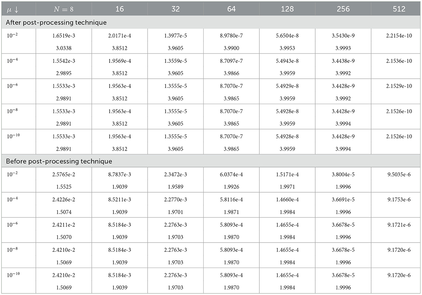
Table 1. Computation of $e_{\epsilon ,\mu }^N,{\left(e_{\epsilon ,\mu }^N\right)}^{post-processed}$ ${\rho }_{\epsilon ,\mu }^N,{\left({\rho }_{\epsilon ,\mu }^N\right)}^{post-processed}$ for Example (1) using ε = 10⁻².

Table 2

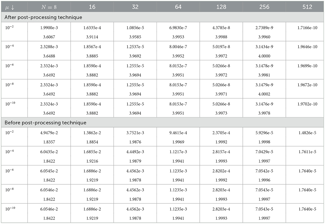
Table 2. Computation of $e_{\epsilon ,\mu }^N,{\left(e_{\epsilon ,\mu }^N\right)}^{post-processed}$ ${\rho }_{\epsilon ,\mu }^N,{\left({\rho }_{\epsilon ,\mu }^N\right)}^{post-processed}$ for Example (2) using ε = 10⁻².

Table 3

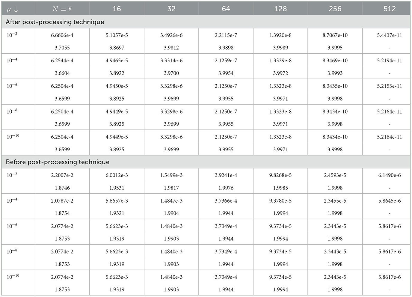
Table 3. Computation of $e_{\epsilon ,\mu }^N,{\left(e_{\epsilon ,\mu }^N\right)}^{post-processed}$ ${\rho }_{\epsilon ,\mu }^N,{\left({\rho }_{\epsilon ,\mu }^N\right)}^{post-processed}$ for Example (3) using ε = 10⁻².

Figure 1

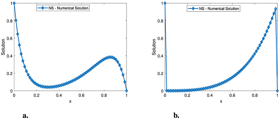
Figure 1. A plot of the numerical solution for Example (1) at N = 64 and μ = 10⁻⁶. (A) ε = 10⁻². (B) ε = 10⁻⁶.

Figure 2

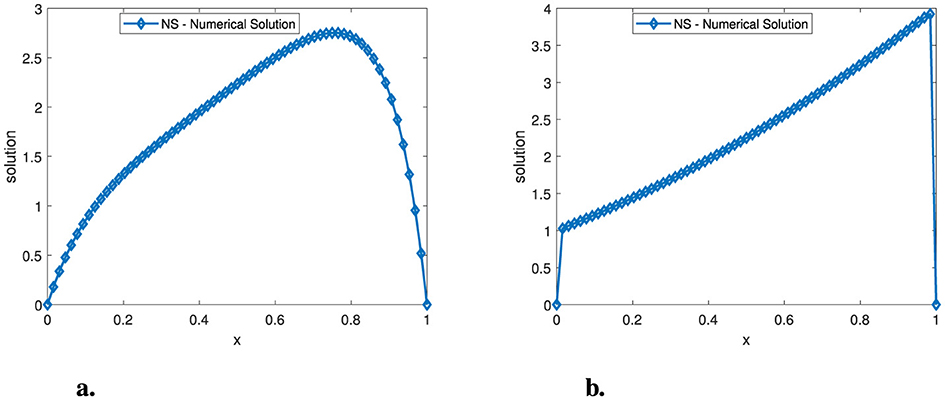
Figure 2. A plot of the numerical solution for Example (2) at N = 64 and μ = 10⁻⁶. (A) ε = 10⁻². (B) ε = 10⁻⁶.

Figure 3

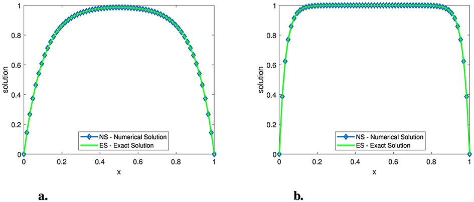
Figure 3. Plot of the numerical solution for Example (3) at N = 64 and μ = 10⁻⁶. (A) ε = 10⁻². (B) ε = 10⁻³.

Figure 4

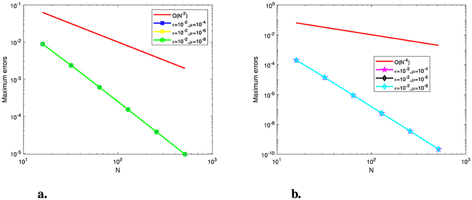
Figure 4. Log-log plot of the maximum point-wise errors for Example (1). (A) Before post-processing. (B) After post-processing.

Figure 5

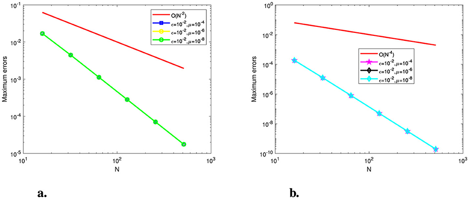
Figure 5. Log-log plot of the maximum point-wise errors for Example (2). (A) Before post-processing. (B) After post-processing.

Figure 6

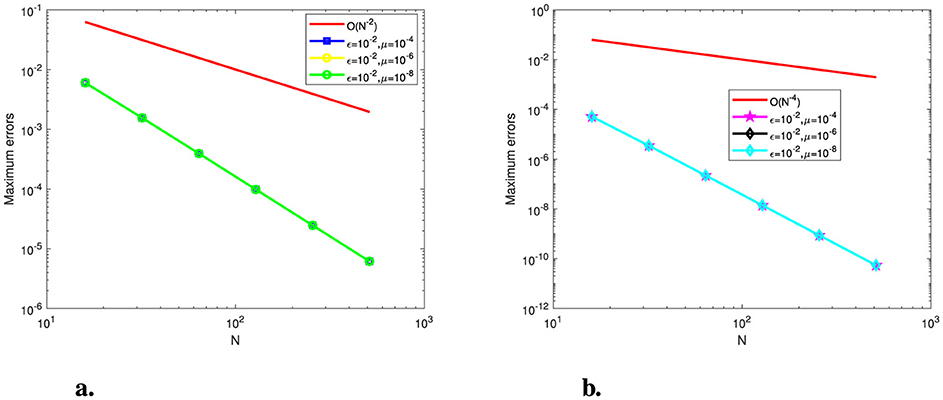
Figure 6. Log-log plot of the maximum point-wise errors for Example (3). (A) Before post-processing. (B) After post-processing.

6 Conclusion

A higher-order exponentially fitted operator finite difference method for two parameter singularly perturbed boundary value problems is presented in this study. The stability and uniform convergence of the current method are well established, ensuring second-order convergence. The post-processing technique is then applied to enhance the convergence order of the method and improve accuracy in terms of maximum errors. Theoretically, we have proven that the post-processing technique provides fourth-order parameter-uniform convergence. Three numerical examples are computed for various perturbation parameter values in order to verify the applicability of the current method. The present method can be applied to singularly perturbed parabolic problem with or without delay.

Data availability statement

The original contributions presented in the study are included in the article/supplementary material, further inquiries can be directed to the corresponding author/s.

Author contributions

AA: Conceptualization, Formal analysis, Investigation, Methodology, Software, Validation, Writing – original draft, Writing – review & editing, Supervision. FG: Conceptualization, Formal analysis, Investigation, Methodology, Software, Supervision, Validation, Writing – original draft, Writing – review & editing. MF: Conceptualization, Investigation, Methodology, Writing – original draft, Writing – review & editing, Software, Supervision.

Funding

The author(s) declare that no financial support was received for the research, authorship, and/or publication of this article.

Acknowledgments

The authors appreciate valuable comments and suggestions of the reviewers.

Conflict of interest

The authors declare that the research was conducted in the absence of any commercial or financial relationships that could be construed as a potential conflict of interest.

Publisher's note

All claims expressed in this article are solely those of the authors and do not necessarily represent those of their affiliated organizations, or those of the publisher, the editors and the reviewers. Any product that may be evaluated in this article, or claim that may be made by its manufacturer, is not guaranteed or endorsed by the publisher.

References

1. Chen J, O'Malley R Jr. On the asymptotic solution of a two-parameter boundary value problem of chemical reactor theory. SIAM J Appl Math. (1974) 26:717–29. doi: 10.1137/0126064

Crossref Full Text | Google Scholar

2. Bigge J, Bohl E. Deformations of the bifurcation diagram due to discretization. Mathem. Comput. (1985) 45:393–403. doi: 10.1090/S0025-5718-1985-0804931-X

PubMed Abstract | Crossref Full Text | Google Scholar

3. DiPrima RC. Asymptotic methods for an infinitely long slider squeeze-film bearing. J Lubr Technol. (1968) 90:173–83. doi: 10.1115/1.3601534

Crossref Full Text | Google Scholar

4. O'Malley R. Two-parameter singular perturbation problems for second-order equations. J. Math. Mech. (1967) 16:1143–64.

Google Scholar

5. Lodhi RK, Jaiswal BR, Nandan D, Ramesh K. Numerical Solution of two-parameter singularly perturbed convection-diffusion boundary value problems via fourth order compact finite difference method. Math Modell Eng Probl. (2021) 8:819–25. doi: 10.18280/mmep.080519

Crossref Full Text | Google Scholar

6. Kambampati S, Emineni SP, Reddy M, Kolloju P. Fourth order computational spline method for two-parameter singularly perturbed boundary value problem. Int J Appl Mech Eng. (2023) 28:79–93. doi: 10.59441/ijame/176516

Crossref Full Text | Google Scholar

7. Pandit S, Kumar M. Haar wavelet approach for numerical solution of two parameters singularly perturbed boundary value problems. Appl Math Inf Sci. (2014) 8:2965. doi: 10.12785/amis/080634

Crossref Full Text | Google Scholar

8. Khandelwal P, Khan A. Singularly perturbed convection-diffusion boundary value problems with two small parameters using nonpolynomial spline technique. Math Sci. (2017) 11:119–26. doi: 10.1007/s40096-017-0215-3

Crossref Full Text | Google Scholar

9. O'Riordan E, Pickett M. Numerical approximations to the scaled first derivatives of the solution to a two parameter singularly perturbed problem. J Comput Appl Math. (2019) 347:128–49. doi: 10.1016/j.cam.2018.08.004

Crossref Full Text | Google Scholar

10. Roos HG, Uzelac Z. The SDFEM for a convection-diffusion problem with two small parameters. Comput Methods Appl Math. (2003) 3:443–58. doi: 10.2478/cmam-2003-0029

Crossref Full Text | Google Scholar

11. Kadalbajoo MK, Yadaw AS. B-Spline collocation method for a two-parameter singularly perturbed convection-diffusion boundary value problems. Appl Math Comput. (2008) 201:504–13. doi: 10.1016/j.amc.2007.12.038

PubMed Abstract | Crossref Full Text | Google Scholar

12. Kadalbajoo MK, Jha A. Exponentially fitted cubic spline for two-parameter singularly perturbed boundary value problems. Int J Comput Math. (2012) 89:836–50. doi: 10.1080/00207160.2012.663492

PubMed Abstract | Crossref Full Text | Google Scholar

13. Brdar M, Zarin H. Convection-diffusion-reaction problems on a B-type mesh. PAMM. (2013) 13:423–4. doi: 10.1002/pamm.201310207

Crossref Full Text | Google Scholar

14. Luo XQ, Liu LB, Ouyang A, Long G. B-spline collocation and self-adapting differential evolution (jDE) algorithm for a singularly perturbed convection-diffusion problem. Soft Computing. (2018) 22:2683–93. doi: 10.1007/s00500-017-2523-9

Crossref Full Text | Google Scholar

15. Brdar M, Zarin H. On graded meshes for a two-parameter singularly perturbed problem. Appl Math Comput. (2016) 282:97–107. doi: 10.1016/j.amc.2016.01.060

Crossref Full Text | Google Scholar

16. Brdar M, Zarin H. A singularly perturbed problem with two parameters on a Bakhvalov-type mesh. J Comput Appl Math. (2016) 292:307–19. doi: 10.1016/j.cam.2015.07.011

Crossref Full Text | Google Scholar

17. Padmaja P, Aparna P, Gorla RSR, Pothanna N. Numerical solution of singularly perturbed two parameter problems using exponential splines. Int J Appl Mech Eng. (2021) 26:160–72. doi: 10.2478/ijame-2021-0025

PubMed Abstract | Crossref Full Text | Google Scholar

18. Andisso FS, Duressa GF. Graded mesh B-spline collocation method for two parameters singularly perturbed boundary value problems. MethodsX. (2023) 11:102336. doi: 10.1016/j.mex.2023.102336

PubMed Abstract | Crossref Full Text | Google Scholar

19. Linß T, Roos HG. Analysis of a finite-difference scheme for a singularly perturbed problem with two small parameters. J Math Anal Appl. (2004) 289:355–66. doi: 10.1016/j.jmaa.2003.08.017

PubMed Abstract | Crossref Full Text | Google Scholar

20. Cheng Y. On the local discontinuous Galerkin method for singularly perturbed problem with two parameters. J Comput Appl Math. (2021) 392:113485. doi: 10.1016/j.cam.2021.113485

Crossref Full Text | Google Scholar

21. Zhang J, Lv Y. High-order finite element method on a Bakhvalov-type mesh for a singularly perturbed convection-diffusion problem with two parameters. Appl Math Comput. (2021) 397:125953. doi: 10.1016/j.amc.2021.125953

Crossref Full Text | Google Scholar

22. Valarmathi S, Ramanujam N. Computational methods for solving two-parameter singularly perturbed boundary value problems for second-order ordinary differential equations. Appl Math Comput. (2003) 136:415–41. doi: 10.1016/S0096-3003(02)00053-X

Crossref Full Text | Google Scholar

23. Patidar KC. A robust fitted operator finite difference method for a two-parameter singular perturbation problem1. J Diff Equ Appl. (2008) 14:1197–214. doi: 10.1080/10236190701817383

Crossref Full Text | Google Scholar

24. Hassen ZI, Duressa GF. Parameter-uniformly convergent numerical scheme for singularly perturbed delay parabolic differential equation via extended B-spline collocation. Front Appl Math Stat. (2023) 9:1255672. doi: 10.3389/fams.2023.1255672

Crossref Full Text | Google Scholar

25. Mohye MA, Munyakazi JB, Dinka TG. A nonstandard fitted operator finite difference method for two-parameter singularly perturbed time-delay parabolic problems. Front Appl Math Stat. (2023) 9:1222162. doi: 10.3389/fams.2023.1222162

Crossref Full Text | Google Scholar

26. Tesfaye SK, Duressa GF, Woldaregay MM, Dinka TG. Fitted computational method for singularly perturbed convection-diffusion equation with time delay. Front Appl Math Stat. (2023) 9:1244490. doi: 10.3389/fams.2023.1244490

Crossref Full Text | Google Scholar

27. Cheru SL, Duressa GF, Mekonnen TB. Numerical integration method for two-parameter singularly perturbed time delay parabolic problem. Front Appl Math Stat. (2024) 10:1414899. doi: 10.3389/fams.2024.1414899

Crossref Full Text | Google Scholar

28. Daba IT, Melesse WG, Kebede GD. Third-degree B-spline collocation method for singularly perturbed time delay parabolic problem with two parameters. Front Appl Math Stat. (2024) 9:1260651. doi: 10.3389/fams.2023.1260651

Crossref Full Text | Google Scholar

29. Gupta V, Kadalbajoo MK, Dubey RK. A parameter-uniform higher order finite difference scheme for singularly perturbed time-dependent parabolic problem with two small parameters. Int J Comput Math. (2019) 96:474–99. doi: 10.1080/00207160.2018.1432856

Crossref Full Text | Google Scholar

30. Gupta V, Sahoo SK, Dubey RK. Robust higher order finite difference scheme for singularly perturbed turning point problem with two outflow boundary layers. Comput Appl Math. (2021) 40:1–23. doi: 10.1007/s40314-021-01564-w

Crossref Full Text | Google Scholar

31. Sahoo SK, Gupta V. A robust uniformly convergent finite difference scheme for the time-fractional singularly perturbed convection-diffusion problem. Comput Math Appli. (2023) 137:126–46. doi: 10.1016/j.camwa.2023.02.016

Crossref Full Text | Google Scholar

32. Ejere AH, Duressa GF, Woldaregay MM, Dinka TG. A robust numerical scheme for singularly perturbed differential equations with spatio-temporal delays. Front Appl Math Stat. (2023) 9:1125347. doi: 10.3389/fams.2023.1125347

Crossref Full Text | Google Scholar

33. Daba IT, Duressa GF. Numerical treatment of singularly perturbed unsteady Burger-Huxley equation. Front Appl Math Stat. (2023) 8:1061245. doi: 10.3389/fams.2022.1061245

PubMed Abstract | Crossref Full Text | Google Scholar

34. Derzie EB, Munyakazi JB, Dinka TG. A NSFD method for the singularly perturbed Burgers-Huxley equation. Front Appl Math Stat. (2023) 9:1068890. doi: 10.3389/fams.2023.1068890

PubMed Abstract | Crossref Full Text | Google Scholar

35. Li J, Singh G, Ilhan OA, Manafian J, Gasimov YS. Modulational instability, multiple Exp-function method, SIVP, solitary and cross-kink solutions for the generalized KP equation. AIMS Math. (2021) 6:7555–84. doi: 10.3934/math.2021441

Crossref Full Text | Google Scholar

36. El Ahmadi M, Ayoujil A, Berrajaa M. Existence and multiplicity of solutions for a class of double phase variable exponent problems with nonlinear boundary condition. Adv Math Models Appl. (2023) 8:401–14.

Google Scholar

37. Nachaoui A. An iterative method for cauchy problems subject to the convection-diffusion equation. Adv Math Models Appl. (2023) 8:327–38.

Google Scholar

38. Mardanov MJ, Sharifov YA, Gasimov YS, Cattani C. Non-linear first-order differential boundary problems with multipoint and integral conditions. Fractal Fract. (2021) 5:15. doi: 10.3390/fractalfract5010015

Crossref Full Text | Google Scholar

39. O'Malley RE. Introduction to Singular Perturbations. New York, NY (1974).

Google Scholar

40. Kellogg RB, Tsan A. Analysis of some difference approximations for a singular perturbation problem without turning points. Math Comput. (1978) 32:1025–39. doi: 10.1090/S0025-5718-1978-0483484-9

PubMed Abstract | Crossref Full Text | Google Scholar