The connection between non-normality and trophic coherence in directed graphs

Abstract

Trophic coherence and non-normality are both ways of describing the overall directionality of directed graphs or networks. Trophic coherence can be regarded as a measure of how neatly a graph can be divided into distinct layers, whereas non-normality is a measure of how unlike a matrix is with its transpose. We explore the relationship between trophic coherence and non-normality by first considering the connections that exist in literature and calculating the trophic coherence and non-normality for some toy networks. We then explore how persistence of an epidemic in an SIS model depends on coherence and how this relates to the non-normality. A similar effect on dynamics governed by a linear operator suggests that it may be useful to extend the concept of trophic coherence to matrices, which do not necessarily represent graphs.

1 Introduction

In this perspective article, we aimed to explore the relationship between trophic coherence and non-normality, which are both qualities used to describe directed graphs. Non-normality refers to the overall asymmetry of an adjacency matrix. Trophic coherence is defined as how neatly the network can be divided into distinct layers, but it can also be interpreted as a tendency of edges to align with a global direction. These two notions come together in directed graphs. A directed graph can be represented with an N × N adjacency matrix A. If the graph is unweighted then A is binary: A_ij = 1 if there is an edge from node v_i to node v_j, else A_ij = 0. When there is an edge from v_i to v_j, we will say that v_i “sees” v_j. A weighted directed graph can be represented with a matrix whose entries are real numbers. For our purposes here, we will always assume that A is non-negative. Each node has an in-degree and an out-degree: and . These are sometimes referred to as “strengths” if the directed graph is weighted.

Definition 1.1. (Non-normality.) Given a real matrix A and its transpose A^T, we say that the matrix A is normal if AA^T−A^TA = 0. It is non-normal otherwise.

Definition 1.2. (Trophic Coherence) A directed graph is said to be maximally coherent if it is possible to assign to each node a natural number such that nodes assigned to n only see others assigned to n + 1. The greater the deviation from such a configuration, the more incoherent the graph.

The need to understand non-normal matrices and operators arises in the fields of fluid dynamics [1–4], PT-symmetry [5–12], and mathematical biology [13] among other disciplines. In particular, non-normal systems are often characterized by eigenvalues that are sensitive to perturbation. It is for this non-normality is considered an asset in information transfer and communication as it can amplify small environmental changes [14, 15]. Additionally, non-normal linear operators are difficult to capture numerically as small discrepancies arising from machine precision can manifest as large perturbations in the eigenvalues. This has given rise to the study of pseudospectra; the ϵ-pseudospectrum of a matrix A is defined as the set {z ∈ ℂ:||(A−zI)⁻¹|| < ϵ⁻¹}). The definition of pseudospectra corresponds to a measure of sensitivity to perturbations of size ϵ; an equivalent definition of pseudospectra is the set {z ∈ Sp(A+B):||B|| ≤ ϵ} [16]. Despite this being one of the most useful tools for understanding how eigenvalues respond to perturbation, it is not necessarily the best way of understanding the sensitivity of directed graphs to operators such as changing the weights of edges or edge deletion. This is equivalent to putting a structure on the matrix B, which thus breaks the correspondence between the “perturbation view of pseudospectra” and the “transient phenomena” view of pseudospectra. The latter is particularly relevant when the adjacency matrix represents a discrete dynamical system.

Ecologists define the “trophic level” of a species as the average level of its prey, plus one [17]. Trophic coherence was first proposed as a solution to May's paradox: the fact that large ecosystems are stable [18]. If the trophic difference of each edge in a graph is the difference between the trophic levels of the in- and out-neighbors, then the broader the distribution of differences (i.e., the larger the standard deviation of this distribution), the more incoherent the network. It was found that ecosystem models based on sufficiently coherent graphs became more stable, rather than less so, with increasing size. It was subsequently shown, by means of graph ensembles and numerical simulations, that trophic coherence could be related to several aspects of directed networks more generally, including the spectral radius and distribution of cycles [19]; motif profiles [20]; non-normality and strong connectivity [21, 22]; pseudospectra [23]; and various dynamical processes [24–26]. However, relying on the ecological definition of trophic levels restricted the application of trophic coherence to networks with at least one node with in-degree zero. Hence, a new measure of trophic levels was proposed that can be applied to any directed graph [27]. This is the method we use here.

In this article, we wish to emphasize the connection between trophic coherence and non-normality and to suggest that this may be relevant not only for directed graphs but for other systems described by matrices. In the first section, “Measuring Trophic Coherence and Non-normality,” we take a deeper look into literature and present results that connect the two ideas. We also calculate the non-normality and trophic coherence of some toy networks in order to help the reader build an intuition. In the second section, we study an SIS model and a simple linear dynamics, both of which are affected by the coherence of an underlying matrix. We see how non-normality, strong connectivity, and the spectral radius also change with the trophic coherence. We then conclude by discussing potential further avenues of research to establish stronger bonds between these topics.

2 Measuring trophic coherence and non-normality

Definition 2.1. The vector of trophic levels h of a directed graph with adjacency matrix A is the solution to the equation

where

and the vectors of total degree and degree imbalance are, respectively, u = kⁱⁿ + k^out and v = kⁱⁿ − k^out [27]. As the solution to Equation 1 is defined only up to an additive constant, the convention that min(h_i) = 0 is used (i.e., all the elements of h are positive except for the smallest value which is set to zero.)

While Equation 1 always has a solution, which is unique given the convention stated at the end of the definition, we should note that one cannot obtain this solution by inverting Λ, as this matrix is always singular. One must therefore use some other method to find the solution, such as LU decomposition, the Moore-Penrose pseudo-inverse or an iterative method.

We can measure the trophic coherence of a directed graph with the incoherence parameterF, given by:

Definition 2.2. The trophic incoherence of a directed graph with adjacency matrix A and trophic levels h given by Equation 1 is as follows:

The incoherence F would coincide with the square of the parameter q proposed by Johnson et al. [18] if trophic levels were calculated as in ecology (F = q²) [18]. Using the trophic levels given by Equation 1, F is bounded between zero and one: F = 0 implies a perfectly coherent directed graph in which vertices fit into integer trophic levels; and F = 1 corresponds to maximum incoherence, which occurs if and only if the directed graph is balanced (v = 0) [27].

Definitions 2.1 and 2.2 were originally derived by first writing down (Equation 3) for generic levels, and then finding the solution h that minimized F—which leads to Equation 1. In other words, the trophic levels, under this definition, are those which minimize the trophic incoherence.

The average trophic difference is z = 1 − F, so one interpretation of trophic coherence is as the “directedness” of the graph, and z can be referred to as the trophic coherence [27]. Another interpretation is given by SpringRank [28], which likens each edge to a spring with natural length l = 1. F is then the energy, which is minimized at the solution h. However, another interpretation of the same equation is Helmholtz-Hodge decomposition, whereby a vector field can be decomposed into a gradient part and a zero divergence part [29]. When applied to graphs, F is then its “circularity.” The fact the same equation has appeared independently at least three times testifies to its wide applicability [27]. We note also that if the “−1” in Equation 3 were replaced with a constant “−a,” this would simply multiply the trophic levels by a: h′ = ah. Hence, a = 1 is a natural choice that does not reduce generality.

Λ is twice the Laplacian of the undirected version of the graph (A + A^T)/2, which can be considered an undirected graph as all edges now have an opposite edge of the same weight. In particular, an interpretation is that Λh = v is the corresponding inhomogenous equation to the homogenous equation (L(A) + L(A^T))x = 0. The multiplicity of the eigenvalue 0 corresponds to the number of connected components in the undirected case, hence can be seen as when we “force” (L(A) + L(A^T))x = 0, by unbalancing the in and out degrees on each node.

Whereas the trophic coherence can be captured by a single number, it is not so easy to have a single number which captures non-normality. Various measures have been proposed to quantify the non-normality of matrices, the most obvious being ||AA^T − A^TA|| for some suitable norm (here and in the paper we use the Frobenius norm). Another method is Henrici's deviation from normality: , where ||·||_F is the Frobenius norm and {λ_i} are the eigenvalues of A. This can be normalized by dividing through by the giving the parameter

is known as the “normality” [27]. Note that a directed graph with normal adjacency matrix A would have and hence ν = 1 (d_F = 0), but a “very non-normal” network would have |λ_j| = 0 for all j and in this case ν = 0 (d_F = 1). However, we stress that the idea of “very non-normal” is also subjective with respect to which measure. The norm ||AA^T − A^TA|| can be considered more sensitive to structural features such as skewness or asymmetry, whereas Henrici's measure aggregates deviations related to eigenvalue magnitudes, potentially smoothing out localized anomalies. In particular, for matrices close to being symmetric, but not normal, the two measures might diverge significantly. The measure ||AA^T − A^TA|| could show a large deviation, while Henrici's measure may remain small if the eigenvalues are unaffected.

In Table 1, we compute the trophic coherence and non-normality measures for two graphs (the loop on five vertices and the so-called vortex graph on five vertices). We consider these measures for both the adjacency matrix and the non-symmetric Laplacian L(A). We also add an edge to the cycle and delete an edge. We see that trophic coherence increases (trophic incoherence F decreases) in both settings. In addition, we can relate back to our previous discussion regarding pseudospectra. where deletion and addition of an edge can be considered a norm of the same size; hence, a more nuanced approach is needed. In addition, we have that the two measures of non-normality behave differently as the Henrici norm perceives the graph with edge deletion as more non-normal regarding the adjacency matrix and the Laplacian, whereas the converse is true for the other measure. Further analysis is needed to establish if there is a physical meaning to this in certain scenarios, i.e., the graph represents a dynamical system. Although, in both cases, the orientation of each edge can be reversed resulting in the same graph, the fact that flow is not conserved on the “loop under edge addition” may make this graph more asymmetric. Further study must be done in this direction to establish this.

Table 1

	Vortex graph on five vertices V5	Loop on five vertices P5	Loop under edge deletion (chain)	Loop under edge addition
Property
Adjacency Matrix
Laplacian (L = Dout−A)
Trophic incoherence (F)	1	1	0	0.91
Trophic levels	(0,0,0,0,0)	(0,0,0,0,0)	(0,1,2,3,4)	(0,0.18, 0.27, 0.36, 0.54)
Adjacency non-normality ||ATA−AAT||	0	0	1.41	2.44
Laplacian non-normality ||LTL−LLT||	0	0	2	4
Adjacency non-normality (Henrici)	0	0	1	0.37
Laplacian non-normality (Henrici)	0	0	0.71	0.38

Comparison of various properties for different types of networks (vortex graph on five vertices, loop on five vertices, loop under edge addition, loop under edge deletion).

Asllani et al. [30] have recently studied the effects of non-normality in directed graphs, where it was shown that d_F correlates strongly with a measure of structural asymmetry. Furthermore, the structures of graphs with different degree distributions were calculated. The approach of the Henrici norm has also been used recently in work looking at non-normality in the context of trophic coherence [21, 27].

It is possible to estimate the expected value of various magnitudes given that a network has a specified trophic coherence, by means of graph ensembles [19, 21, 27]. The “coherence ensemble” is the set of all possible directed graphs with a given degree sequence and trophic coherence. Thus, the expected value of the spectral radius is as follows:

and the bar denotes expectation [19]. L is the number of edges, L_B is the number of edges connected to the source or sink nodes (those with no incoming or outgoing edges), and the “branching factor” is α = 〈kⁱⁿk^out〉/〈k〉 where the brackets are averages over vertices. τ is referred to as the “loop exponent.” Because τ is positive for F ≃ 1 but becomes negative when F ≃ 0, directed graphs fall into one of two regimes, referred to as “loopful” (τ > 0) and “loopless” (τ < 0) [19]. In the former the number of circuits of length l increases exponentially with l, whereas in the latter they decay exponentially. This can have a crucial bearing on many other topological and dynamical features of complex systems, as we illustrate below with the example of an SIS model: an epidemic perdures indefinitely when τ > 0 but quickly goes extinct when τ < 0.

This approach has been used to show that the expected non-normality is bounded, [21], and approximated by [27]. Hence, trophically coherent graphs (F → 0 or τ → −∞) are non-normal (d_F → 1). The fact that the expected value of the non-normality is bounded below by the expected spectral radius [21] is natural when considering the transient wave-packet phenomena that can happen with non-normal matrices [16].

3 Spreading processes with graphs and operators

It is known that the trophic coherence of directed graphs can exert an important influence on the dynamics of various complex systems [21]. Similarly, in dynamical systems governed by linear operators, the non-normality thereof will fundamentally affect system behavior [16]. We go on to show, using two simple examples of spreading processes, that there are close similarities between these two kinds of phenomena. First we look at the SIS model on coherent directed graphs and then we compare this to the action of a non-normal linear operator. These examples also show that the methods which have been proposed to generate directed graphs with tunable trophic coherence might also be useful for studying other matrices numerically [24, 31].

The SIS (susceptible-infectious-susceptible) model is perhaps the simplest which can be used to study the spread through a population of an infectious disease—typically one which confers little or no immunity [32]. We will use this paradigm to demonstrate the influence of trophic coherence or non-normality on even the simplest of dynamical processes.

Consider an unweighted, directed network given by the N × N adjacency matrix A. To each node i is associated with a dynamical variable s_i(t) which can take, at each discrete time t, either the value 0 or 1, representing susceptible or infectious states, respectively. Let . The system then evolves according to:

with all nodes updated in parallel. In other words, a susceptible node becomes infectious for one time step if at least one of its in-neighbors is infectious.

Will an epidemic die out naturally or go on indefinitely? We study this by beginning with all nodes being susceptible except for %5 which are chosen at random to be made infectious. We generate networks using the generalized preferential preying model [24]. This model has a parameter, T, which allows one to set the trophic coherence of the network: T = 0 produces maximally coherent structures, and incoherence increases with positive T.

Not that in this scheme the only randomness is in the generation of the network and the choice of initial conditions; the dynamics thereafter are deterministic. Figure 1 top left shows the stationary proportion of nodes which remain infectious indefinitely against T. At low values of T the epidemic dies out, but for higher values, there is a continuous transition to a regime in which a significant proportion of the nodes remain infectious. This can be understood by considering that the epidemic requires a strongly connected component of nodes to sustain itself, which only exists in sufficiently incoherent networks [22]. Or, more formally, it is known that the critical rate of infection required for an epidemic to survive is lower bounded by the inverse of the spectral radius of the adjacency matrix [33], which depends on trophic coherence [19].

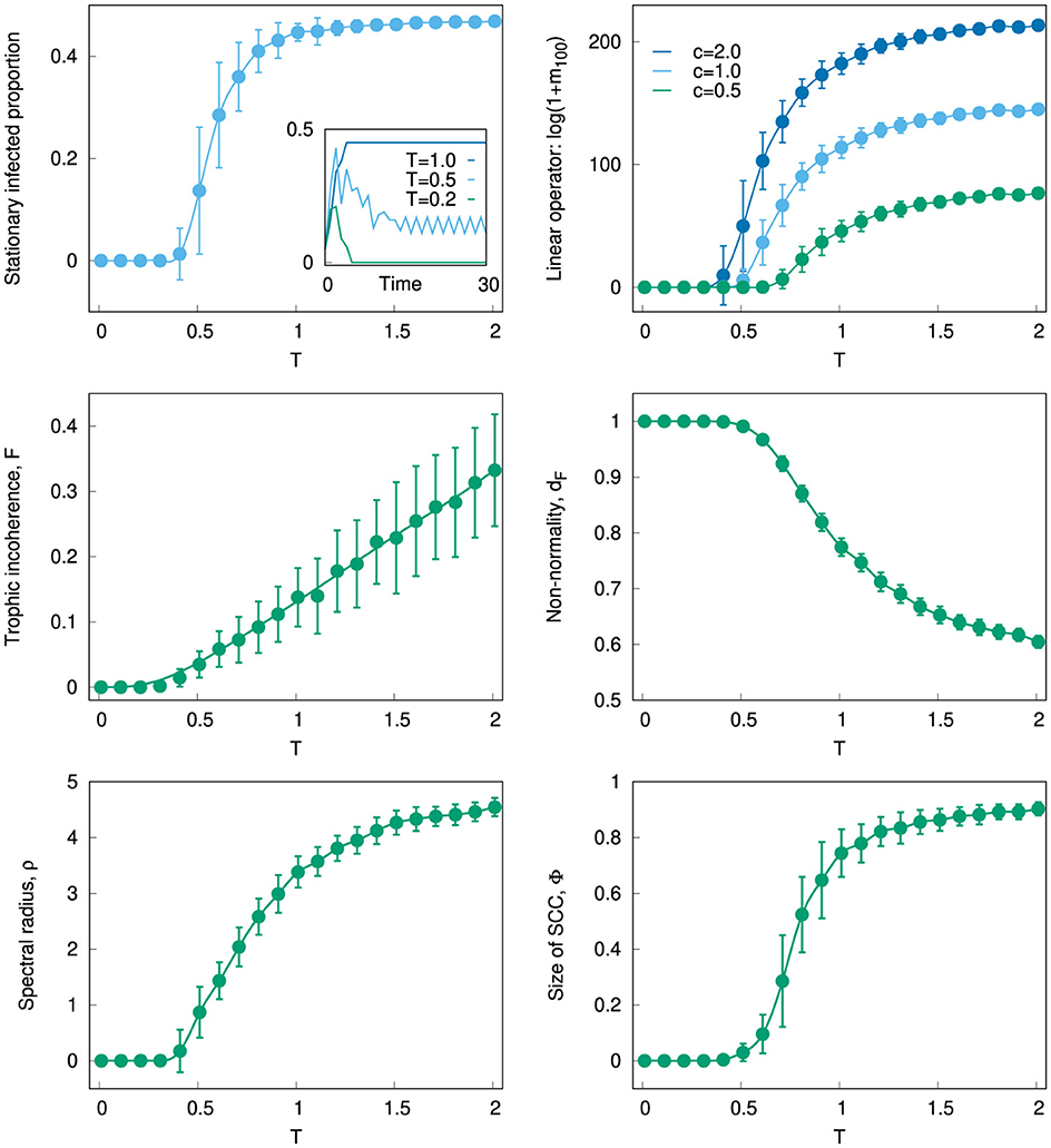
Figure 1

24]. Number of nodes and edges: N = 100 and L = 500. Averages over 100 networks; error bars are standard deviations. Stationary values computed as the average from t = 90 to t = 100. Inset: Time series of the proportion of infected nodes for three networks, generated with T = 1, 0.5, and 0.2. Top right: Mean activity m(t) at t = 100 according to Equations 8, 9, where A is the adjacency matrix of the networks used in the top left panel. Initially, all elements have x(0) = 0, except for a randomly chosen 5% which are set to x(0) = 1. The extent of activity is measured as ln[1 + m(100)], for c = 0.5, 1, and 2. Middle left: Trophic incoherence F against T for the same directed graphs as in the panels above. Middle right: Non-normality d_F against T for the same directed graphs. Bottom left: Spectral radius ρ against T for the same directed graphs. Bottom right: Size of the strongly connected component Φ against T for the same directed graphs.

As we have seen, non-normality also varies with trophic coherence. Hence, in the inset we see a “bump” in the time series for lower values of T (which produces small F and high d_F), which corresponds to transient phenomena. In a future study, we will consider the average difference between the pseudospectral abscissa and the spectral radius at early times to establish transient phenomena [16]. In our SIS model computations, we see that as trophic coherence increases, the size of the strongly-connected component increases. Unlike in undirected graphs, the multiplicity of the λ = 0 eigenvalue of the Laplacian L(A) does not equal the number of components, but rather the number of reaches [34] (a reach is the maximal unilaterally connected set). Whereas dynamical processes such as these have been related to the existence and size of strongly connected components, we have yet to investigate the effect of different reach structures.

Consider now the following dynamical system with N elements. Every element i is characterized by a continuous dynamical variable x_i(t) at discrete time t. The system evolves according to

where c is a constant parameter and A is a non-negative, N × N real matrix. We might consider A as a linear operator or as a directed graph on which the process is taking place. In particular, we can take A to be infinite dimensional in which case we could be giving a graphical interpretation to such linear operators. We begin with a small number of randomly chosen agents in state x(0) = 1 and all others x(0) = 0, and track the average value of the activity,

This will either decay to zero or diverge according to the spectral radius of A and the parameter c, as shown in Figure 1 top right. However, for significantly non-normal networks (low T) there may be transient behavior that eventually dies out, as in the SIS case on a trophically coherent graph. This might correspond to an epidemic, rumor or other spreading process, which reaches most of the system but goes on to disappear, whereas in the more normal or incoherent case, even a process that only reaches some of the system might continue to fuel itself indefinitely thanks to feedback.

Figure 1 middle left, middle right shows how the trophic incoherence F and the non-normality d_F also vary in this network model with the parameter T. A comparison with Figure 1 top left reveals that some nodes begin to sustain the epidemic once F>0 or d_F < 1; and a similar effect is evident in the linear operator case (Figure 1 top right). Figure 1 bottom left, bottom right shows how the two topological features we can relate to both the SIS dynamic and the linear operator – namely, the spectral radius ρ and the size of the strongly connected component Φ—undergo a similar transition with increasing T as the stationary proportion of infected nodes or the logarithm of m(t). Just as degree heterogeneity can drastically reduce the size of epidemic waves [35], trophic coherence can affect their extinction. Moreover, whereas trophic coherence has to date been thought of only as a property of directed graphs, this example suggests that it can be studied in the case of operators and square matrices more broadly.

4 Discussion

In this article, we have discussed the relationship between trophic coherence and non-normality. We have mentioned some existing connections in the literature and studied some small graphs for illustration. We have also presented numerical experiments in the form of an SIS model and a linear dynamics, which show how trophic coherence and non-normality are related and have significant effects on dynamical systems governed by matrices.

There are many relationships still to be discovered, particularly regarding the connection between non-normality and trophic coherence in matrices in general. Also of interest is the relationship with strongly connected components, and how edge deletion and edge addition may be considered in a way that is amenable to the calculation of pseudospectra. In future work, we aim to explore which kind of edge perturbations can create the largest change in non-normality, trophic coherence, or even other measures such as algebraic connectivity (which is non-trivial to compute in a directed graph and is so far yet to profit from the advances in the computations of non-self-adjoint problems). By studying how such edge perturbations change the non-normality, trophic coherence, and algebraic connectivity, we may improve our understanding of how such magnitudes are related and their effects on dynamical systems. This is the subject of upcoming study.

References

• 1.

  CossuCChomazJM. Global measures of local convective instabilities. Phys Rev Lett. (1997) 78:4387. 10.1103/PhysRevLett.78.4387

  • CrossRef
  • Google Scholar
  • View reference in article

• 2.

  ChomazJM. Global instabilities in spatially developing flows: non-normality and nonlinearity. Annu Rev Fluid Mech. (2005) 37:357–92. 10.1146/annurev.fluid.37.061903.175810

  • CrossRef
  • Google Scholar
  • View reference in article

• 3.

  SujithRJuniperMSchmidP. Non-normality and nonlinearity in thermoacoustic instabilities. Int J Spray Combust Dyn. (2016) 8:119–46. 10.1177/1756827716651571

  • CrossRef
  • Google Scholar
  • View reference in article

• 4.

  SchmidPJHenningsonDSJankowskiD. Stability and transition in shear flows. Applied mathematical sciences, vol 142. Appl Mech Rev. (2002) 55:B57–9. 10.1115/1.1470687

  • CrossRef
  • Google Scholar

• 5.

  BenderCMBrodyDCJonesHF. Complex extension of quantum mechanics. Phys Rev Lett. (2002) 89:270401. 10.1103/PhysRevLett.89.270401

  • Pubmed Abstract
  • CrossRef
  • Google Scholar

• 6.

  BenderCM. Making sense of non-Hermitian Hamiltonians. Rep Prog Phys. (2007) 70:947–1018. 10.1088/0034-4885/70/6/R03

  • Pubmed Abstract
  • CrossRef
  • Google Scholar
  • View reference in article

• 7.

  BenderCMBoettcherS. Real spectra in non-Hermitian Hamiltonians having PT symmetry. Phys Rev Lett. (1998) 80:5243–6. 10.1103/PhysRevLett.80.5243

  • CrossRef
  • Google Scholar
  • View reference in article

• 8.

  BenderCMBrodyDCJonesHF. Must a Hamiltonian be Hermitian?Am J Phys. (2003) 71:1095–102. 10.1119/1.1574043

  • CrossRef
  • Google Scholar
  • View reference in article

• 9.

  BenderCMMeisingerPNWangQ. Calculation of the hidden symmetry operator in PT-symmetric quantum mechanics. J Phys A Math Gen. (2003) 36:1973–83. 10.1088/0305-4470/36/7/312

  • CrossRef
  • Google Scholar
  • View reference in article

• 10.

  MostafazadehA. Metric operator in pseudo-Hermitian quantum mechanics and the imaginary cubic potential. J Phys A Math Gen. (2006) 39:10171–88. 10.1088/0305-4470/39/32/S18

  • CrossRef
  • Google Scholar
  • View reference in article

• 11.

  SieglPKrejčiříkD. On the metric operator for the imaginary cubic oscillator. Phys Rev D. (2012) 86:121702. 10.1103/PhysRevD.86.121702

  • CrossRef
  • Google Scholar
  • View reference in article

• 12.

  DaviesEB. Wild spectral behaviour of anharmonic oscillators. Bull Lond Math Soc. (2000) 32:432–8. 10.1112/S0024609300007050

  • CrossRef
  • Google Scholar
  • View reference in article

• 13.

  DrysdaleCColbrookMJ. A novel use of pseudospectra in mathematical biology: understanding HPA axis sensitivity. arXiv preprint arXiv:240800845. (2024).

  • Google Scholar
  • View reference in article

• 14.

  BaggioGZampieriS. Non-normality improves information transmission performance of network systems. IEEE Trans Control Netw Syst. (2021) 8:1846–58. 10.1109/TCNS.2021.3088795

  • CrossRef
  • Google Scholar
  • View reference in article

• 15.

  BaggioGRuttenVHennequinGZampieriS. Efficient communication over complex dynamical networks: the role of matrix non-normality. Sci Adv. (2020) 6:eaba2282. 10.1126/sciadv.aba2282

  • Pubmed Abstract
  • CrossRef
  • Google Scholar
  • View reference in article

• 16.

  TrefethenLNEmbreeM. Spectra and Pseudospectra: The Behavior of Nonnormal Matrices and Operators. Princeton: Princeton University Press. (2005). 10.1515/9780691213101

  • CrossRef
  • Google Scholar
  • View reference in article

• 17.

  LevineS. Several measures of trophic structure applicable to complex food webs. J Theor Biol. (1980) 83:195–207. 10.1016/0022-5193(80)90288-X

  • Pubmed Abstract
  • CrossRef
  • Google Scholar
  • View reference in article

• 18.

  JohnsonSDomínguez-GarcíaVDonettiLMuñozMA. Trophic coherence determines food-web stability. Proc Natl Acad Sci. (2014) 111:17923–8. 10.1073/pnas.1409077111

  • Pubmed Abstract
  • CrossRef
  • Google Scholar
  • View reference in article

• 19.

  JohnsonSJonesNS. Looplessness in networks is linked to trophic coherence. Proc Natl Acad Sci USA. (2017) 114:5618–23. 10.1073/pnas.1613786114

  • Pubmed Abstract
  • CrossRef
  • Google Scholar
  • View reference in article

• 20.

  KlaiseJJohnsonS. The origin of motif families in food webs. Sci Rep. (2017) 7:16197. 10.1038/s41598-017-15496-1

  • Pubmed Abstract
  • CrossRef
  • Google Scholar
  • View reference in article

• 21.

  JohnsonS. Digraphs are different: Why directionality matters in complex systems. J Phys. (2020) 1:015003. 10.1088/2632-072X/ab8e2f

  • CrossRef
  • Google Scholar
  • View reference in article

• 22.

  RodgersNTiňoPJohnsonS. Strong connectivity in real directed networks. Proc Natl Acad Sci. (2023) 120:e2215752120. 10.1073/pnas.2215752120

  • Pubmed Abstract
  • CrossRef
  • Google Scholar
  • View reference in article

• 23.

  RodgersNTiňoPJohnsonS. Influence and influenceability: global directionality in directed complex networks. R Soc Open Sci. (2023) 10:221380. 10.1098/rsos.221380

  • Pubmed Abstract
  • CrossRef
  • Google Scholar
  • View reference in article

• 24.

  KlaiseJJohnsonS. From neurons to epidemics: How trophic coherence affects spreading processes. Chaos. (2016) 26:065310. 10.1063/1.4953160

  • Pubmed Abstract
  • CrossRef
  • Google Scholar
  • View reference in article

• 25.

  PilgrimCGuoWJohnsonS. Organisational social influence on directed hierarchical graphs, from tyranny to anarchy. Sci Rep. (2020) 10:1–13. 10.1038/s41598-020-61196-8

  • Pubmed Abstract
  • CrossRef
  • Google Scholar
  • View reference in article

• 26.

  RodgersNTiňoPJohnsonS. Network hierarchy and pattern recovery in directed sparse Hopfield networks. Phys Rev E. (2022) 105:064304. 10.1103/PhysRevE.105.064304

  • Pubmed Abstract
  • CrossRef
  • Google Scholar
  • View reference in article

• 27.

  MacKayRSJohnsonSSansomB. How directed is a directed network?R Soc Open Sci. (2020) 7:201138. 10.1098/rsos.201138

  • Pubmed Abstract
  • CrossRef
  • Google Scholar
  • View reference in article

• 28.

  De BaccoCLarremoreDBMooreC. A physical model for efficient ranking in networks. Sci Adv. (2018) 4:eaar8260. 10.1126/sciadv.aar8260

  • Pubmed Abstract
  • CrossRef
  • Google Scholar
  • View reference in article

• 29.

  KichikawaYIyetomiHIinoTInoueH. Community structure based on circular flow in a large-scale transaction network. Appl Netw Sci. (2019) 4:1–23. 10.1007/s41109-019-0202-8

  • CrossRef
  • Google Scholar
  • View reference in article

• 30.

  AsllaniMLambiotteRCarlettiT. Structure and dynamical behavior of non-normal networks. Sci Adv. (2018) 4:eaau9403. 10.1126/sciadv.aau9403

  • Pubmed Abstract
  • CrossRef
  • Google Scholar
  • View reference in article

• 31.

  RodgersNTiňoPJohnsonS. Fitness-based growth of directed networks with hierarchy. J Phys. (2024) 5:035013. 10.1088/2632-072X/ad744e

  • CrossRef
  • Google Scholar
  • View reference in article

• 32.

  HethcoteHW. Three basic epidemiological models. In: Applied Mathematical Ecology. Springer (1989). p. 119–144. 10.1007/978-3-642-61317-3_5

  • CrossRef
  • Google Scholar
  • View reference in article

• 33.

  Van MieghemPVan de BovenkampR. Non-Markovian infection spread dramatically alters the susceptible-infected-susceptible epidemic threshold in networks. Phys Rev Lett. (2013) 110:108701. 10.1103/PhysRevLett.110.108701

  • Pubmed Abstract
  • CrossRef
  • Google Scholar
  • View reference in article

• 34.

  VeermanJLyonsRA. primer on Laplacian dynamics in directed graphs. Nonlinear Phenom Compl Syst. (2020) 23:196–206. 10.33581/1561-4085-2020-23-2-196-206

  • CrossRef
  • Google Scholar
  • View reference in article

• 35.

  JohnsonS. Epidemic modelling requires knowledge of the social network. J Phys. (2024) 5:01LT01. 10.1088/2632-072X/ad19e0

  • CrossRef
  • Google Scholar
  • View reference in article