Laplacian spectra and structural insights: applications in chemistry and network science

This paper presents the practical applications of Laplacian and signless Laplacian spectra across various fields including theoretical chemistry, computer science, electrical engineering, and complex network analysis. By focusing on the spectrum-based evaluation of generalized mesh network and ladder graphs, the research aims to uncover valuable relationships with the structural properties of real-world networks. The study not only explores the theoretical underpinnings but also applies these spectra to calculate essential network measures such as mean-first passage time, average path length, spanning trees, and spectral radius. These analyses offer a deeper understanding of how graph spectra influence network characteristics, enriching our ability to predict and analyze complex networks. This comprehensive approach enhances our knowledge across multiple scientific disciplines, facilitating more informed predictions about drugs infrastructure.

1 Introduction

Spectral graph theory is an important part of algebraic graph theory which mainly utilizes matrix theory, polynomial theory, and combinatorial methods to study the different spectra (or ranges of values) that come from graphs. Furthermore, spectral theory investigates how these spectra are connected to the structure and properties of graphs. It links the algebraic (math-based) aspects of graphs to their topological (shape-based) aspects. By studying how a graph's spectrum relates to its structure, we can not only better understand these graphs but also find useful applications in areas like improving networks, designing computer circuits, and solving operational problems. Some key areas of study in spectral theory include the adjacency spectrum, Laplacian spectrum, signless-Laplacian spectrum, and distance spectrum of graphs. Among these, the Laplacian spectrum is the most studied and produces the most results. Studying the Laplacian spectrum is not only valuable for theoretical knowledge but also has many uses in chemistry, physics, complex networks, and electronic engineering. Over the last few decades, significant attention has been given to examining the structure of graphs, along with their spectral, topological, and combinatorial characteristics. Laplacian eigenvalues have proven useful in identifying various graph invariants, including the Kirchhoff index, global mean-first passage time, and the count of spanning trees. Typically, the characteristic polynomial and spectrum of the graph matrix for certain graph operations, such as the complement, union, Cartesian product, direct product, and strong product, can be derived from the factor graphs. Since complex molecular graphs can be effectively described using graph operations, it is feasible to represent the properties of these complex molecular graphs through the invariants of their factor graphs.

From the perspective of spectral graph theory, numerous structural features and dynamic behaviors of graphs have been investigated. The literature on spectral graph theory covers diverse aspects of Laplacian matrices across different graph structures. Merris provides a comprehensive survey, discussing the Laplacian matrix's spectrum, algebraic connectivity, and applications in areas such as chemistry [1]. Hong and Zhang investigate Laplacian eigenvalues in simple and bipartite graphs, establishing key bounds and structural insights, particularly for trees and regular graphs [2]. Agaev and Chebotarev (2006) extended the study to weighted directed graphs, exploring the connections between Laplacian and stochastic matrices and their semiconvergent properties [3]. Rojo and Soto focused on unweighted rooted trees, analyzing the eigenvalues of adjacency and Laplacian matrices based on symmetric tridiagonal matrices [4]. Ding and Jiang investigate the spectral norms and eigenvalue distributions of random graph matrices, revealing key convergence behaviors aligned with Wigner's semi-circular law [5]. Wu extends the use of Laplacian matrices into quantum mechanics, exploring conditions for separability in weighted graphs [6]. Kaveh and Rahami (2006) focus on the eigenvalues and eigenvectors of graph products, presenting efficient methods for solving eigenproblems in structural mechanics, especially for Cartesian and lexicographic products [7]. Spielman emphasizes the significance of Laplacian matrices in algorithm design, highlighting their role in fast solutions for linear equations and their application to graph theory through innovations like graph sparsifiers and local clustering [8].

In 2012, Estrada introduced path Laplacian matrices as a new concept that generalized the combinatorial Laplacian and applied them to consensus analysis in networks, thus showing its potential for enhancing network synchronization and other applications [9]. In their 2013 publication, Krishnan et al. came up with a novel scheme of multi-level preconditioning for Laplacian matrices used in computer graphics which resulted in substantial performance benefits in applications such as image colorization and mesh processing [10]. Another similar work by Dong et al. aimed toward exploring laplacian matrix learning for smooth graph signal representation that contributed to advancement in graph signal processing [11]. Pirani and Sundaram analyzed the smallest eigenvalue properties of grounded Laplacian matrices giving out insights into spectral graph theory and its applications [12]. Efficient methods have been developed by Bergamaschi and Martínez to approximate the generalized inverse of Laplacian matrices which are important when solving large scale graph problems [13]. Recent research on Laplacian matrices has led to notable advancements. In 2016, Jog and Kotambari analyzed the spectra of coalesced complete graphs, studying the adjacency, Laplacian, and signless Laplacian energies to understand their spectral properties and applications [19]. Moving to 2018, Bandeira explored random Laplacian matrices, revealing that the largest eigenvalue often approximates the largest diagonal entry, with implications for convex relaxation techniques and Erdos-Rényi graph connectivity thresholds [14]. Li provided insights into the constrained Rayleigh quotient for eigen-balanced Laplacian matrices, which proved valuable for cooperative control problems and convergence rates in consensus protocols [16]. The work by Bergamaschi and Bozzo focused on comparing algorithms for computing the smallest eigenpairs of graph Laplacians, including the Implicitly Restarted Lanczos Method and Jacobi-Davidson method, particularly for large, sparse networks [18]. Zhou et al. introduced an optimal neighborhood multi-view spectral clustering algorithm, which enhances clustering performance by effectively combining first-order and high-order Laplacian matrices [15]. Hermann and Konigorski addressed the optimization of edge weights in directed graph Laplacians to achieve desired spectral properties [17].

In 2019, Alhevaz et al. explored the Brouwer-type conjecture related to the eigenvalues of the distance signless Laplacian matrix. Their findings provided bounds for the sums of the largest and smallest eigenvalues, applying these results to graphs with specific diameters and transmission properties [20]. Moving forward to 2022, Ganie and Shang investigated the spectral radius and energy of the signless Laplacian matrix of digraphs, proposing new lower bounds and characterizing extremal digraphs based on vertex degrees and walk lengths [21]. Also in 2022, Morbidi examined matrix functions of the Laplacian matrix and their applications to distributed formation control, showing how these functions can enhance performance and flexibility in consensus protocols [22]. Recent studies have significantly advanced our understanding of various Laplacian matrices and their applications. In 2021, Reinhart introduced the normalized distance Laplacian matrix, offering new insights into its spectral properties and connections with the normalized Laplacian matrix. The study showed that this matrix has fewer cospectral pairs compared to other matrices [23]. The same year, Chakrabarty et al. explored the spectral properties of adjacency and Laplacian matrices in inhomogeneous Erdõs-Rényi random graphs. Their work detailed the empirical spectral distributions and their convergence to deterministic limits [24].

The paper by Alazemi et al. [25] explores chain graphs, a specific class of bipartite graphs, with unique Laplacian eigenvalues. The authors provide structural insights, degree constraints, and analyze the eigenspaces of these graphs. Notably, they highlight conditions such as the absence of vertex triplets sharing identical neighborhoods and propose applications in Laplacian dynamics, including the controllability of multi-agent systems. Meanwhile, Anđelić et al. [26] introduce a family of tridiagonal matrices with eigenvalues as perfect squares, applying this result to analyze the Laplacian controllability of half graphs, a subclass of chain graphs, further advancing the understanding of spectral graph theory. The authors in [28] investigate the Laplacian controllability of graphs formed using standard graph products, including joins, Cartesian, tensor, and strong products. The study provides theoretical insights and introduces an iterative method to construct infinite families of controllable Laplacian pairs. Additionally, Anđelić et al. [29] focus on the Q-index, the largest eigenvalue of the signless Laplacian matrix, for connected graphs with fixed order and size. The authors derive spectral bounds for the Q-index of nested split graphs, offering both theoretical results and computational comparisons to improve understanding of spectral properties in graph theory.

More recently, in 2023, Bapat et al. extended the concept of bipartite matrices by examining the bipartite Laplacian matrix of nonsingular trees. They provided a combinatorial description of this matrix and established several key identities [27]. Additionally, Mallik expanded the Matrix Tree Theorem to signed graphs, introducing a new oriented incidence matrix and offering a combinatorial formula for the determinant of the signless net Laplacian matrix [30]. Raza et al. focused on generalized prism graphs and found that spectral analysis helps measure network features like passage time and path length [31]. Raza and Munir extended this by showing how Laplacian and signless Laplacian spectra can be used to understand network properties and predict behaviors in various fields [32]. In a later study, Raza et al. applied these methods to torus grid graphs, deriving key network measures and improving our knowledge of network structures [33].

We define a path of length α_m ∈ ℕ as the graph P_αm that has vertex set V = {v ∈ ℕ : 0 ≤ v ≤ α_m} and where two vertices determine an edge if and only if |v_i−v_j| = 1 for v_i, v_j ∈ V. Then, a mesh network graph ${\mathcal{M}}_m^n$, often known as two-dimensional lattice graph or grid graph, is defined as the Cartesian product ${\mathcal{M}}_m^n=P_{{\alpha }_m}⊡P_{{\alpha }_n}$, exhibits a total of 2mn−m−n = (m−1)n+(n−1)m edges, reflecting the combined count of horizontal and vertical edges. Simultaneously, ${\mathcal{M}}_m^n$ boasts mn vertices, aligning with the Cartesian product of the vertex sets of P_m and P_n. The mentioned graph operation have gained significant attention in the field of graph theory and computer science. These graphs are widely used to model spatial relationships and connectivity in various applications, such as computer networks, image processing, and computational geometry. The study of grid graphs has evolved over the years, with researchers exploring their properties, algorithms, and applications. Harel and Sardashti [34] presented a comprehensive analysis of the structural characteristics of mesh network graph, highlighting their regularity and symmetry. Smith et al. [35] investigated efficient algorithms for computing shortest paths in mesh network graphs, providing valuable insights into optimizing navigation in grid-based environments. Additionally, Chen and Du [36] explored the application of ${\mathcal{M}}_m^n$ in wireless sensor networks, showcasing their relevance in practical scenarios. Recent work by Hinz and Holz auf der Heide [35] delved into the dynamic aspects, addressing challenges related to real-time updates and adaptability. Furthermore, the survey by Kumar et al. [37] offers a holistic overview of mesh network graph applications and algorithmic advancements. Building on earlier research about mesh network graphs and their spectra, our study thoroughly examined the Adjacency et al. Laplacian spectra of ${\mathcal{M}}_m^n$. We didn't just calculate these spectra; we also applied them to real-world network analysis. Using our results, we computed important network measures such as graph energies, Kirchhoff index, mean-first passage time, path length, spanning trees, and spectral radius. This approach aimed to give a deeper insight into the properties of ${\mathcal{M}}_m^n$, such as its connectivity, resilience, and efficiency. In this section, we review key findings from earlier studies that relate to the solutions discussed in this paper. This study distinguishes itself by conducting a comprehensive spectral analysis of generalized mesh networks, focusing on the adjacency, Laplacian, and signless Laplacian spectra to derive explicit expressions for critical network parameters such as the Kirchhoff index, spectral radius, average path length, global mean first passage time, graph energies, and the number of spanning trees. While previous research has applied spectral methods to various network types, such as torus networks and categorical product networks, your work uniquely emphasizes generalized mesh networks, providing detailed spectral characterizations that enhance the understanding of their structural and dynamic properties. The complete structure of our article is presented hierarchically in Figure 1. By presenting results graphically, your study offers clear visualizations of how these parameters vary with network dimensions, facilitating deeper insights into their interplay and impact. This approach not only broadens the applicability of spectral methods but also offers a robust framework for exploring and optimizing complex real-world networks, thereby contributing valuable perspectives across multiple scientific disciplines.

Figure 1

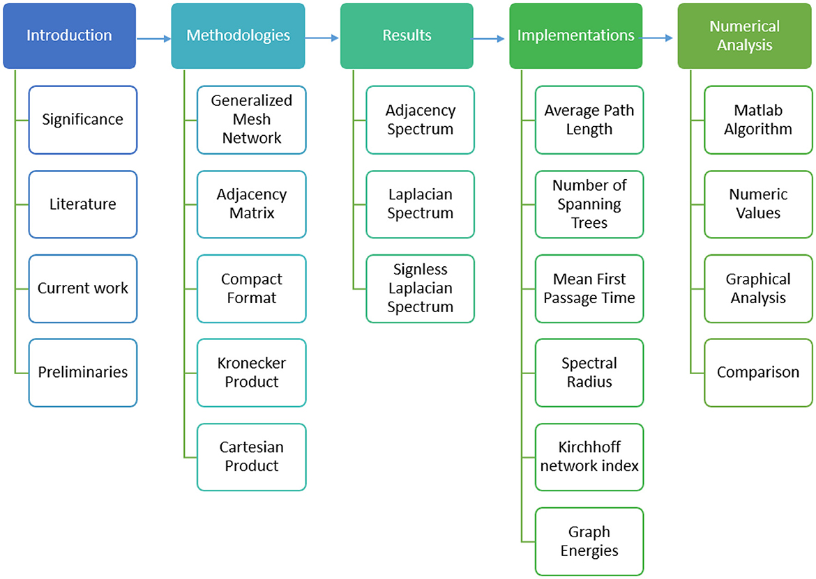
Figure 1. Structuring the research: a detailed map of the paper's content.

2 Preliminaries

Before discussing graph-based matrices and the related lemmas associated with the Kronecker product, let's first revisit the notion of ψ-sum graphs. Let $ = (V($), E($)) be a simple undirected graph, where V($) represents its vertex set and E($) represents its edge set. The number of vertices in $ is denoted by |V($)|, and the number of edges is denoted by |E($)|. If an edge e connects two vertices u and v, the edge uv can also be referred to as e. For a given vertex v ∈ V($), its neighborhood in $, denoted by N_$(v), is the set of vertices adjacent to v, specifically N_$(v) = {u ∈ V($)∣uv ∈ E($)}. The degree of a vertex v, symbolized as d_$(v), is the number of vertices in its neighborhood, i.e., d_$(v) = |N_$(v)|.

Definition 1. The diagonal matrix is defined as ${\mathcal{D}}_g(\$)=\mathrm{\text{diag}}\left[d_{{\upsilon }_{ij}}\right]$ for i = j and the Laplacian matrix ${\mathcal{L}}_p(\$)={\mathcal{D}}_g(\$)-{\mathcal{A}}_d(\$)$ is defined by the subtraction of the adjacency matrix from the diagonal matrix of vertex degrees. Elaborating in matrix form, ${\mathcal{L}}_p(\$)$ is defined as:

$\begin{array}{l}{ℒ}_p(\text{\$})=\{\begin{array}{l}-1\text{ for all }{\upsilon }_i⊵{\upsilon }_j,\hfill \\ d_{{\upsilon }_{ij}}\text{ for all }i=j,\hfill \\ 0\text{ for all }{\upsilon }_i⋭{\upsilon }_j.\hfill \end{array}\end{array}$

Lemma 1. Let E ∈ M_{p, p}(G), F ∈ M_{p, q}(G), G ∈ M_{q, p}(G), H ∈ M_{q, q}(G) with H being invertible, such that

$T=\left(\begin{array}{ll}E\hfill & F\hfill \\ G\hfill & H\hfill \end{array}\right)$

Then,

$det(T)=det(H)-det(E-F{H}^{-1}G)$

Lemma 2. Let C = (c_ij) ∈ M_{r, s}(G), D ∈ M_{t, u}(G). Then the Kronecker product of C and D is defined as

$C\otimes D=\left(\begin{array}{cccc}{c}_{11}D& c_{12}D& \cdots & c_{1r}D\\ c_{21}D& c_{22}D& \cdots & c_{2r}D\\ ⋮& ⋮& \ddots & ⋮\\ c_{s1}D& c_{s2}D& \cdots & c_{sr}D\end{array}\right)$

Lemma 3. Let C and D be square matrices of order r and s, respectively, with eigenvalues λ_i (1 ≤ i ≤ r) and ν_j (1 ≤ j ≤ s). Then the eigenvalues of C ⊗ I_s+I_r ⊗ D are λ_i+ν_j. Moreover, if V_i is an eigenvector of C corresponding to λ_i and W_j is an eigenvector of D corresponding to ν_j, then V_i ⊗ W_j is an eigenvector of C ⊗ I_s+I_r ⊗ D corresponding to λ_i+ν_j.

Lemma 4. Let C ∈ M_{r, s}(G), D ∈ M_{t, u}(G), E ∈ M_{r, t}(G), F ∈ M_{s, u}(G), and β ∈ G. The following properties hold:

(a) (C ⊗ D)^T = C^T ⊗ D^T.

(b) (C ⊗ D)(E ⊗ F) = (CE) ⊗ (DF).

(c) (C ⊗ D) ⊗ E = C ⊗ (D ⊗ E).

(d) β(C ⊗ D) = βC ⊗ D = C ⊗ βD.

(e) If C and D are invertible, then (C ⊗ D)⁻¹ = C⁻¹ ⊗ D⁻¹.

Lemma 5. The eigenvalues of the Adjacency matrix, Laplacian matrix, and Signless Laplacian matrix for a path graph ${\mathcal{P}}_n$ are expressed as $2cos\left(\frac{\pi k}{n+1}\right)$, $2-2cos\left(\frac{\pi k}{n}\right)$, and $2+2cos\left(\frac{2\pi k}{n+1}\right)$, respectively, where k = 0, 1, 2, …, n−1.

3 Methodologies and results

In this section, we have evaluated the exact values for the Adjacency, Laplacian and signless Laplacian spectrum of the generalized Mesh Network graphs utilizing the graph and algebra techniques. Theorem 1 provides expressions for the sum of reciprocals and the product of adjacency eigenvalues of the generalized mesh graph ${\mathcal{M}}_m^n$, which are fundamental in understanding network connectivity and robustness [38]. The sum of the reciprocals of the eigenvalues is often associated with resistance distance and other network invariants, while their product is related to graph determinant properties, which have applications in quantum networks and structural analysis [39]. Extending this analysis, Theorem 2 focuses on the Laplacian eigenvalues, which play a crucial role in describing network dynamics such as diffusion processes and synchronization [41]. The sum of the reciprocals of the Laplacian eigenvalues is connected to important network measures like Kirchhoff's index, influencing resistance-based properties, while their product is associated with the number of spanning trees, a key quantity in evaluating network reliability and resilience [42]. Furthermore, Theorem 3 explores the Signless Laplacian spectrum, which is particularly useful in applications involving directed flows and energy distribution in networks [40]. The sum of the reciprocals of these eigenvalues helps in analyzing clustering tendencies in complex networks, whereas their product provides a measure of structural stability and modular properties. These interpretations establish strong connections between spectral properties and real-world applications, enhancing the accessibility of the results for researchers in diverse fields such as physics, computer science, and engineering.

Theorem 1. Let the summation of the reciprocals and the product of the adjacency eigenvalues of the generalized mesh graph ${\mathcal{M}}_m^n$ be denoted by ${\mathcal{Z}}_m^n$ and ${\mathcal{W}}_m^n$, respectively. Then:

$\begin{array}{l}{\mathcal{Z}}_m^n=\frac{1}{2}{\displaystyle \sum _{j=0}^{m-1}}{\displaystyle \sum _{i=0}^{n-1}}{\left(cos\frac{\pi i}{n+1}+cos\frac{\pi j}{m+1}\right)}^{-1}\end{array}$

$\begin{array}{l}{\mathcal{W}}_m^n=2{\displaystyle \prod _{j=0}^{m-1}}{\displaystyle \prod _{i=0}^{n-1}}\left(cos\frac{\pi i}{n+1}+cos\frac{\pi j}{m+1}\right)\end{array}$

Proof. The adjacency matrix of the mesh graph ${\mathcal{M}}_m^n$ is:

$ℬ\left({ℳ}_m^n\right)={\left[\begin{array}{ccc}{I}_n& & \text{\hspace{1em}if }k=\ell -1\text{ and }k\ge 1,\\ ℬ\left(Q_n\right)& & \text{\hspace{1em}if }k=\ell ,\\ I_n& & \text{\hspace{1em}if }k=\ell +1\text{and}k\ge 2,\\ O_n& & \text{\hspace{1em}otherwise}.\end{array}\right]}_m,$

By matrix addition, it can be expressed as:

$\begin{array}{l}ℬ\left({ℳ}_m^n\right)={\left[\begin{array}{ccc}ℬ\left(Q_n\right)& & \text{\hspace{1em}for }k=\ell ,\\ O_n& & \text{\hspace{1em}otherwise}.\end{array}\right]}_m\\ +{\left[\begin{array}{ccc}{I}_n& & \text{\hspace{1em}if }k\ge 1,\ell =k+1\text{ or }k\ge 2,\ell =k-1,\\ O_n& & \text{\hspace{1em}otherwise}.\end{array}\right]}_m.\end{array}$

Using Lemma 2, we have:

$\begin{array}{l}ℬ\left({ℳ}_m^n\right)={\left[\begin{array}{cc}1& \text{\hspace{1em}for }k=\ell ,\\ O_m& \text{\hspace{1em}otherwise}.\end{array}\right]}_m\otimes ℬ\left(Q_n\right)\\ +{\left[\begin{array}{cc}1& \text{\hspace{1em}for }k\ge 1,\ell =k+1\text{or}k\ge 2,\ell =k-1,\\ O_m& \text{\hspace{1em}otherwise}.\end{array}\right]}_m\otimes I_n.\end{array}$

The matrix

${\left[\begin{array}{cc}1& \text{\hspace{1em}for }k\ge 1,\ell =k+1\text{or}k\ge 2,\ell =k-1,\\ O_m& \text{\hspace{1em}otherwise}.\end{array}\right]}_m$

is the adjacency matrix of Q_m, a path graph with m vertices. Thus:

$\mathcal{B}\left({\mathcal{M}}_m^n\right)=\mathcal{B}\left(Q_n\right)\otimes I_m+\mathcal{B}\left(Q_m\right)\otimes I_n.$

Now, assume two invertible matrices U and V related to the matrices Q_n and Q_m, such that:

$\mathcal{B}{\left(Q_n\right)}^{\prime }=U^{-1}\mathcal{B}\left(Q_n\right)U,$

and

$\mathcal{B}{\left(Q_m\right)}^{\prime }=V^{-1}\mathcal{B}\left(Q_m\right)V,$

Since, the eigenvalues of the Adjacency matrix for a path graph Q_n are given by ${\lambda }_k=2cos\left(\frac{\pi k}{n+1}\right),k=0,1,2,\dots ,n-1,$ so the diagonal entries of the upper triangular matrices are:

$\begin{array}{l}2cos\frac{\pi i}{n+1},\text{and\hspace{1em}}2cos\frac{\pi j}{m+1},\text{with\hspace{1em}}i=0,1,\dots ,n-1\\ \text{and\hspace{1em}}j=0,1,\dots ,m-1.\end{array}$

Consequently:

$\begin{array}{l}{\left(U\otimes V\right)}^{-1}\left(\mathcal{B}\left(Q_n\right)\otimes I_m+\mathcal{B}\left(Q_m\right)\otimes I_n\right)\left(U\otimes V\right)\\ =\mathcal{B}{\left(Q_n\right)}^{\prime }\otimes I_m+\mathcal{B}{\left(Q_m\right)}^{\prime }\otimes I_n,\end{array}$

and the diagonal entries of this upper triangular matrix are given by:

$\begin{array}{l}2\left(cos\frac{\pi i}{n+1}+cos\frac{\pi j}{m+1}\right),\text{with\hspace{1em}}i=0,1,\dots ,n-1\\ \text{and\hspace{1em}}j=0,1,\dots ,m-1.\end{array}$

Thus, the adjacency eigenvalues for the generalized mesh graph are:

$\begin{array}{l}2cos\frac{\pi i}{n+1}+2cos\frac{\pi j}{m+1},\text{with\hspace{1em}}i=0,1,\dots ,n-1\\ \text{and\hspace{1em}}j=0,1,\dots ,m-1.\end{array}$

Using this result, we obtain:

${\mathcal{Z}}_m^n=\frac{1}{2}{\displaystyle \sum _{j=0}^{m-1}}{\displaystyle \sum _{i=0}^{n-1}}{\left(cos\frac{\pi i}{n+1}+cos\frac{\pi j}{m+1}\right)}^{-1},$

and

${\mathcal{W}}_m^n=2{\displaystyle \prod _{j=0}^{m-1}}{\displaystyle \prod _{i=0}^{n-1}}\left(cos\frac{\pi i}{n+1}+cos\frac{\pi j}{m+1}\right).$

Corollary 1. For a mesh graph with equal dimensions (n = m), the product and sum of the reciprocals of the adjacency eigenvalues are given by:

${\mathcal{Z}}_n^n=\frac{1}{4}{\displaystyle \sum _{j=0}^{n-1}}sec\frac{\pi j}{n+1},\text{and\hspace{1em}}{\mathcal{W}}_n^n=4{\displaystyle \prod _{j=0}^{n-1}}cos\frac{\pi j}{n+1}.$

The proof follows directly from Theorem 1.

Theorem 2. Let ${\mathcal{Z}}_n^m\mathcal{L}$ and ${\mathcal{W}}_n^m\mathcal{L}$ denote the sum of the reciprocals and the product of the Laplacian eigenvalues, respectively, for the generalized mesh network graph ${\mathcal{M}}_m^n$. Then, these quantities are given by:

$\begin{array}{l}{\mathcal{Z}}_n^m\mathcal{L}={\displaystyle \sum _{j=0}^{n-1}}{\displaystyle \sum _{i=0}^{m-1}}{\left(4-2cos\frac{\pi i}{m}-2cos\frac{\pi j}{n}\right)}^{-1},\end{array}$

and

$\begin{array}{l}{\mathcal{W}}_n^m\mathcal{L}=2{\displaystyle \prod _{j=0}^{n-1}}{\displaystyle \prod _{i=0}^{m-1}}\left(2-cos\frac{\pi i}{m}-cos\frac{\pi j}{n}\right).\end{array}$

Proof. The Laplacian matrix associated with the mesh network graph ${\mathcal{M}}_m^n$ is expressed as:

${ℒ}_q\left({ℳ}_m^n\right)={\left[\begin{array}{ccc}-I_m& & \text{if }j=i-1,\text{ when }i\ge 1,\\ {ℒ}_q\left(Q_m\right)& & \text{if }j=i,\\ -I_m& & \text{if }j=i+1,\text{ when }i\ge 2,\\ O_m& & \text{elsewhere}.\end{array}\right]}_n.$

By decomposing this matrix, it can be rewritten as:

$\begin{array}{l}{ℒ}_q\left({ℳ}_m^n\right)={\left[\begin{array}{ccc}{ℒ}_q\left(Q_m\right)& & \text{for }j=i,\\ O_m& & \text{elsewhere}.\end{array}\right]}_n\\ +{\left[\begin{array}{ccc}-I_m& & \text{if }j=i+1\text{ when }i\ge 1\\ -I_m& & \text{if }j=i-1\text{ when }i\ge 2,\\ {\delta }_i& & \text{if }j=i,\\ O_m& & \text{elsewhere}.\end{array}\right]}_n.\end{array}$

Referring to Lemma 2, this is further simplified as:

$\begin{array}{l}={\left[\begin{array}{cc}1& \text{\hspace{1em}for }j=i,\\ O_m& \text{\hspace{1em}elsewhere}.\end{array}\right]}_n\otimes {ℒ}_q\left(Q_m\right)\\ +{\left[\begin{array}{ccc}-1& & \text{if }j=i+1\text{ when }i\ge 1\\ -1& & \text{if }j=i-1\text{ when }i\ge 2,\\ {\delta }_i& & \text{if }j=i,\\ [O_m& & \text{elsewhere}.\end{array}\right]}_n\otimes I_m.\end{array}$

The matrix

${\left[\begin{array}{ccc}-1& & \text{if }j=i+1\text{ when }i\ge 1\text{ or }j=i-1\text{ when }i\ge 2,\\ {\delta }_i& & \text{if }j=i,\\ O_m& & \text{elsewhere}.\end{array}\right]}_n$

is the Laplacian matrix for the path graph Q_n with n nodes. Therefore:

$\begin{array}{l}{\mathcal{L}}_q\left({\mathcal{M}}_m^n\right)={\mathcal{L}}_q\left(Q_m\right)\otimes I_n+{\mathcal{L}}_q\left(Q_n\right)\otimes I_m.\end{array}$

Suppose U and V are invertible matrices related to the matrices Q_n and Q_m, respectively. Then:

$\begin{array}{l}{\left({\mathcal{L}}_q\left(Q_m\right)\right)}^{\prime }=U^{-1}{\mathcal{L}}_q\left(Q_m\right)U,\text{and\hspace{1em}}{\left({\mathcal{L}}_q\left(Q_n\right)\right)}^{\prime }=V^{-1}{\mathcal{L}}_q\left(Q_n\right)V,\end{array}$

Since, The eigenvalues of the Laplacian matrix for a path graph Q_n are given by ${\mu }_k=2-2cos\left(\frac{\pi k}{n}\right),k=0,1,2,\dots ,n-1,$ so the diagonal entries of the upper triangular matrices are:

$\begin{array}{l}2-2cos\frac{\pi i}{m}\text{and\hspace{1em}}2-2cos\frac{\pi j}{n},\end{array}$

where i = 0, 1, 2, …, m−1 and j = 0, 1, 2, …, n−1.

Clearly:

$\begin{array}{l}{\left(U\otimes V\right)}^{-1}\left({\mathcal{L}}_q\left(Q_m\right)\otimes I_n+{\mathcal{L}}_q\left(Q_n\right)\otimes I_m\right)\left(U\otimes V\right)\\ ={\mathcal{L}}_q{\left(Q_m\right)}^{\prime }\otimes I_n+{\mathcal{L}}_q{\left(Q_n\right)}^{\prime }\otimes I_m,\end{array}$

with diagonal elements of the resulting matrix given by:

$\begin{array}{l}4-2cos\frac{\pi i}{m}-2cos\frac{\pi j}{n},\end{array}$

where i = 0, 1, 2, …, m−1 and j = 0, 1, 2, …, n−1.

Thus, the eigenvalues of the Laplacian matrix for the mesh network graph are:

$\begin{array}{ll}4-2\left(cos\frac{\pi i}{m}+cos\frac{\pi j}{n}\right),& \left(1\right)\end{array}$

where i = 0, 1, 2, …, m−1 and j = 0, 1, 2, …, n−1.

Finally, using the eigenvalues in Equation 1, we derive:

$\begin{array}{l}{\mathcal{Z}}_n^m\mathcal{L}={\displaystyle \sum _{j=0}^{n-1}}{\displaystyle \sum _{i=0}^{m-1}}{\left(4-2cos\frac{\pi i}{m}-2cos\frac{\pi j}{n}\right)}^{-1},\end{array}$

and

$\begin{array}{l}{\mathcal{W}}_n^m\mathcal{L}=2{\displaystyle \prod _{j=0}^{n-1}}{\displaystyle \prod _{i=0}^{m-1}}\left(2-cos\frac{\pi i}{m}-cos\frac{\pi j}{n}\right).\end{array}$

Corollary 2. For a mesh network graph of equal dimensions (n = m), the product and reciprocal of the sum of the Laplacian eigenvalues are given by:

${\mathcal{Z}}_n^n\mathcal{L}={\displaystyle \sum _{i=0}^{n-1}}{\left(4-4cos\frac{\pi i}{n}\right)}^{-1},\text{and }{\mathcal{W}}_n^n\mathcal{L}={\displaystyle \prod _{i=0}^{n-1}}\left(4-4cos\frac{\pi i}{n}\right).$

The proof follows directly from Theorem 2.

Theorem 3. Let the sum of the reciprocals and the product of all Signless Laplacian eigenvalues of the generalized mesh graph ${\mathcal{M}}_m^n$ be denoted by ${\mathcal{S}}_n^m\mathcal{Q}$ and ${\mathcal{P}}_n^m\mathcal{Q}$, respectively. Then,

$\begin{array}{l}{\mathcal{S}}_n^m\mathcal{Q}=\frac{1}{2}{\displaystyle \sum _{j=0}^{n-1}}{\displaystyle \sum _{i=0}^{m-1}}{\left(2+cos\frac{2\pi i}{m+1}+cos\frac{2\pi j}{n+1}\right)}^{-1},\end{array}$

$\begin{array}{l}{\mathcal{P}}_n^m\mathcal{Q}=2{\displaystyle \prod _{j=0}^{n-1}}{\displaystyle \prod _{i=0}^{m-1}}\left(2+cos\frac{2\pi i}{m+1}+cos\frac{2\pi j}{n+1}\right).\end{array}$

Proof. The Signless Laplacian matrix for the mesh graph ${\mathcal{M}}_m^n$ is expressed as:

$Q_S\left({ℳ}_m^n\right)={\left[\begin{array}{ccc}{I}_m& & i=j-1,\text{ if }i\ge 1,\\ Q_S\left(P_m\right)& & \text{if }j=i,\\ I_m& & i=j+1,\text{ if }i\ge 2,\\ O_m& & \text{otherwise}\end{array}\right]}_n,$

which can be broken down by matrix addition as follows:

$\begin{array}{l}{Q}_S\left({ℳ}_m^n\right)={\left[\begin{array}{ccc}{Q}_S\left(P_m\right)& & \text{for }i=j,\\ O_m& & \text{otherwise}\end{array}\right]}_n\\ +{\left[\begin{array}{ccc}{I}_m& & \text{if }i\ge 1,j=i+1\text{ or }i\ge 2,j=i-1,\\ d_i& & \text{if }i=j,\\ O_m& & \text{otherwise}\end{array}\right]}_n.\end{array}$

According to Lemma 1.1, we have:

$\begin{array}{l}{Q}_S\left({ℳ}_m^n\right)={\left[\begin{array}{cc}1& \text{for }i=j,\\ O_m& \text{elsewhere}\end{array}\right]}_n\otimes Q_S\left(P_m\right)\\ +{\left[\begin{array}{ccc}1& \text{if }i\ge 1,j=i+1\text{ or }i\ge 2,j=i-1,& \\ d_i& & \text{if }i=j,\\ O_m& & \text{elsewhere}\end{array}\right]}_n\\ \otimes I_m.\end{array}$

The matrix given by

${\left[\begin{array}{ccc}1& \text{if }i\ge 1,j=i+1\text{ or }i\ge 2,j=i-1,& \\ d_i& & \text{if }i=j,\\ O_m& & \text{elsewhere}\end{array}\right]}_n,$

is, in fact, the Signless Laplacian matrix of the path graph P_n with n vertices. Thus, we obtain:

$\begin{array}{l}{\mathcal{Q}}_S\left({\mathcal{M}}_m^n\right)={\mathcal{Q}}_S\left(P_m\right)\otimes I_n+{\mathcal{Q}}_S\left(P_n\right)\otimes I_m.\end{array}$

Introducing two invertible matrices A and B that correspond to the matrices P_n and P_m, we have:

$\begin{array}{l}{\left({\mathcal{Q}}_S\left(P_m\right)\right)}^{\prime }=A^{-1}{\mathcal{Q}}_S\left(P_m\right)A,\end{array}$

and

$\begin{array}{l}{\left({\mathcal{Q}}_S\left(P_n\right)\right)}^{\prime }=B^{-1}{\mathcal{Q}}_S\left(P_n\right)B.\end{array}$

Since, the eigenvalues of the Signless Laplacian matrix for a path graph Q_n are given by $q_k=2+2cos\left(\frac{2\pi k}{n+1}\right),k=0,1,2,\dots ,n-1$ so the diagonal entries of the upper triangular matrices are:

$\begin{array}{l}2+2cos\frac{2\pi i}{m+1}\text{ and }2+2cos\frac{2\pi j}{n+1},\end{array}$

where i = 0, 1, 2, …, m−1 and j = 0, 1, 2, …, n−1.

Clearly, the following holds:

$\begin{array}{l}{\left(A\otimes B\right)}^{-1}\left({\mathcal{Q}}_S\left(P_m\right)\otimes I_n+{\mathcal{Q}}_S\left(P_n\right)\otimes I_m\right)\left(A\otimes B\right)\\ ={\mathcal{Q}}_S{\left(P_m\right)}^{\prime }\otimes I_n+{\mathcal{Q}}_S{\left(P_n\right)}^{\prime }\otimes I_m,\end{array}$

where the diagonal elements of this matrix are given by:

$\begin{array}{l}4+2cos\frac{2\pi i}{m+1}+2cos\frac{2\pi j}{n+1},\end{array}$

where i = 0, 1, 2, …, m−1 and j = 0, 1, 2, …, n−1.

Thus, the adjacency eigenvalues for the mesh graph can be expressed as:

$\begin{array}{ll}2\left(2+cos\frac{2\pi i}{m+1}+cos\frac{2\pi j}{n+1}\right),& \left(2\right)\end{array}$

where i = 0, 1, 2, …, m−1 and j = 0, 1, 2, …, n−1.

From the results in Equation 3, we can derive:

$\begin{array}{l}{\mathcal{S}}_n^m\mathcal{Q}={\displaystyle \sum _{j=0}^{n-1}}{\displaystyle \sum _{i=0}^{m-1}}{\frac{1}{\lambda }}_{j,i}\\ =\frac{1}{2}{\displaystyle \sum _{j=0}^{n-1}}{\displaystyle \sum _{i=0}^{m-1}}{\left(2+cos\frac{2\pi i}{m+1}+cos\frac{2\pi j}{n+1}\right)}^{-1},\\ \left(j,i\right)\ne \left(0,0\right).\end{array}$

and

$\begin{array}{l}{\mathcal{P}}_n^m\mathcal{Q}={\displaystyle \prod _{j=0}^{n-1}}{\displaystyle \prod _{i=0}^{m-1}}{\lambda }_{j,i}=2{\displaystyle \prod _{j=0}^{n-1}}{\displaystyle \prod _{i=0}^{m-1}}\left(2+cos\frac{2\pi i}{m+1}+cos\frac{2\pi j}{n+1}\right),\\ \left(j,i\right)\ne \left(0,0\right).\end{array}$

Corollary 3. For regular dimension mesh graph (n = m), the products and reciprocals of the sums of Signless Laplacian eigenvalues are defined as

$\begin{array}{l}{\mathcal{X}}_n^n\mathcal{Q}={\displaystyle \sum _{\nu =0}^{n-1}}{\left(4+2cos\frac{2\pi \nu }{n+1}\right)}^{-1},\\ \text{and}{\mathcal{Y}}_n^n\mathcal{Q}={\displaystyle \prod _{\nu =0}^{n-1}}\left(4+2cos\frac{2\pi \nu }{n+1}\right).\end{array}$

The proof is obvious by Theorem 3.

4 Laplacian spectra and implementations in networking

The framework developed in the previous section allows for the calculation of important network metrics, including graph energy, Kirchhoff index $\mathcal{K}\mathcal{I}$, spectral radius $\mathcal{S}\mathcal{R}$, average path length $\mathcal{A}\mathcal{P}\mathcal{L}$, global mean first passage time $\mathcal{M}\mathcal{F}\mathcal{T}$, and the number of spanning trees $\mathcal{T}\mathcal{N}$. To facilitate these computations, two key quantities, ${\mathcal{M}}_A$ and ${\mathcal{M}}_B$, are introduced. The quantity ${\mathcal{M}}_A$ is defined as the product of all non-zero eigenvalues, denoted as λ_i, of a given matrix, while ${\mathcal{M}}_B$ is the sum of the reciprocals of these eigenvalues:

${\mathcal{M}}_A={\displaystyle \prod _{i=1}^n}{\lambda }_i\text{and\hspace{1em}}{\mathcal{M}}_B={\displaystyle \sum _{i=1}^n}\frac{1}{{\lambda }_i}.$

Here, λ_i represents the eigenvalues of the Laplacian matrix associated with the graph ${\mathcal{M}}_m^n$, where i ranges from 1 to n. These quantities serve as the basis for further analysis and provide a deeper understanding of various network properties.

4.1 Average path length

The networks with an extremely short mean path length, often referred to as "Small-world" networks, are common in real-world applications. This trait is frequently observed, and various parameters, such as the clustering coefficient, mean path length, and degree distribution, serve as strong indicators of the network's structure. Specifically, for a given mesh graph ${\mathcal{M}}_m^n$, the average path length, denoted by $\mathcal{A}\mathcal{P}\mathcal{L}$, is defined as the average number of steps along the shortest path d_ij. This metric is essential for measuring the efficiency of material transport or information exchange between all possible node pairs within the network. For the network ${\mathcal{M}}_m^n$, $\mathcal{A}\mathcal{P}\mathcal{L}$ is given by:

$\mathcal{APL}\left({\mathcal{M}}_m^n\right)=\frac{2}{n\left(n-1\right)}{\displaystyle \sum _{i<j}}{g}_{ij}\left({\mathcal{M}}_m^n\right).$

In an electrical network modeled as a complete graph, there exists a notable connection between the shortest paths $d_{ij}\left({\mathcal{M}}_m^n\right)$ and the effective resistance $g_{ij}\left({\mathcal{M}}_m^n\right)$, as detailed in reference [43]:

$d_{ij}=\frac{2g_{ij}}{n}.$

Here, n represents the order of the complete graph ${\mathcal{M}}_m^n$, which is the total number of vertices. By combining the equations above, a simplified expression is derived that reveals the relationship within the graph:

$\begin{array}{l}\mathcal{A}\mathcal{P}\mathcal{L}\left({\mathcal{M}}_m^n\right)=\frac{2}{n\left(n-1\right)}·\frac{n}{2}{\displaystyle \sum _{i<j}}\frac{1}{{\lambda }_{ij}}=\frac{n}{n-1}·{\displaystyle \sum _{i<j}}\frac{1}{{\lambda }_{ij}}\\ =\frac{nm}{2\left(nm-1\right)}{\displaystyle \sum _{i=0}^{n-1}}{\displaystyle \sum _{j=0}^{m-1}}{\left(2-cos\frac{\pi j}{m}-cos\frac{\pi i}{n}\right)}^{-1}.\end{array}$

Corollary 4. For a ladder graph, denoted as ${\mathcal{M}}_m^2$, the average path length $\mathcal{A}\mathcal{P}\mathcal{L}\left({\mathcal{M}}_m^2\right)$ can be derived from the general formula for the mesh graph by setting n = 2. The expression for the average path length of the ladder graph is given by:

$\mathcal{A}\mathcal{P}\mathcal{L}\left({\mathcal{M}}_m^2\right)=\frac{1}{\left(2m-1\right)}{\displaystyle \sum _{i=0}^1}{\displaystyle \sum _{j=0}^{m-1}}{\left(2-cos\frac{\pi j}{m}-cos\frac{\pi i}{2}\right)}^{-1}.$

4.2 The number of spanning trees

The count of spanning trees ($\mathcal{T}\mathcal{N}$) plays a crucial role in various complex network phenomena, including random walks, network reliability, resistor networks, transport systems, loop-erased random walks, and self-organized criticality, as explored in studies like [44–47]. Kirchhoff's Matrix-Tree Theorem, as detailed in [48, 49], reveals a fundamental link by showing that the product of all nonzero eigenvalues of a graph's Laplacian matrix equals the total number of spanning trees. This theorem is a powerful tool for accurately computing $\mathcal{T}\mathcal{N}$ for a generalized mesh graph, denoted by $\mathcal{T}\mathcal{N}\left({\mathcal{M}}_m^n\right)$. Essentially, this method provides an efficient way to decipher the intricate connections within the graph, greatly aiding in the precise determination of spanning trees across different network configurations:

$\begin{array}{l}\mathcal{T}\mathcal{N}\left({\mathcal{M}}_m^n\right)=\frac{{\displaystyle {\prod }_{i=2}^n}{\lambda }_i}{n}=\frac{{\displaystyle {\prod }_{i=0}^{m-1}}{\displaystyle {\prod }_{j=0}^{n-1}}{\eta }_{i,j}}{n}\\ =\frac{2}{nm}{\displaystyle \prod _{i=0}^{m-1}}{\displaystyle \prod _{j=0}^{n-1}}\left(2-cos\frac{\pi j}{n}-cos\frac{\pi i}{m}\right).\end{array}$

Corollary 5. For a ladder graph, denoted as ${\mathcal{M}}_m^2$, the number of spanning trees $\mathcal{T}\mathcal{N}\left({\mathcal{M}}_m^2\right)$ can be obtained by setting n = 2 in the general formula for the number of spanning trees of the mesh graph. The expression for the ladder graph is:

$\mathcal{T}\mathcal{N}\left({\mathcal{M}}_m^2\right)=\frac{1}{m}{\displaystyle \prod _{i=0}^{m-1}}{\displaystyle \prod _{j=0}^1}\left(2-cos\frac{\pi j}{2}-cos\frac{\pi i}{m}\right).$

4.3 Global mean-first passage time

In network analysis, the global mean-first passage time ($\mathcal{G}\mathcal{M}\mathcal{F}\mathcal{T}$) is a key metric for assessing the speed of random walks in complex networks, offering insights into how rapidly information or entities travel through the network. It is calculated by averaging individual first passage times over all node pairs. The formula for $\mathcal{G}\mathcal{M}\mathcal{F}\mathcal{T}$ is:

$\mathcal{G}\mathcal{M}\mathcal{F}\mathcal{T}=\frac{1}{n\left(n-1\right)}{\displaystyle \sum _{i=1}^n}{\displaystyle \sum _{j\ne i}^n}{F}_{i,j},$

where F_{i, j} is the first passage time from node i to node j, and n is the total number of nodes. This average is normalized to include all unique pairs. The commuting time (${\mathcal{C}}_{i,j}$) between nodes i and j is given by:

${\mathcal{C}}_{i,j}=F_{i,j}+F_{j,i}=2R_{i,j},$

where R_{i, j} is a graph-specific metric. For a generalized mesh graph ${\mathcal{M}}_m^n$, the global mean-first passage time is computed as:

$\mathcal{G}\mathcal{M}\mathcal{F}\mathcal{T}=\frac{2\mathcal{N}}{n\left(n-1\right)}{\displaystyle \sum _{i<j}}\frac{1}{{\lambda }_{i,j}},$

where n = nm and $\mathcal{N}=2nm-n-m$. Thus, $\mathcal{G}\mathcal{M}\mathcal{F}\mathcal{T}$ becomes:

$\mathcal{G}\mathcal{M}\mathcal{F}\mathcal{T}=\frac{2\left(2nm-n-m\right)}{nm\left(nm-1\right)}{\displaystyle \sum _{i=0}^{m-1}}{\displaystyle \sum _{j=0}^{n-1}}{\left(2-cos\frac{\pi j}{n}-cos\frac{\pi i}{m}\right)}^{-1}.$

Corollary 6. By setting n = 2 in the formula for the global mean-first passage time of a generalized mesh network, we obtain the corresponding result for the ladder graph:

$\mathcal{G}\mathcal{M}\mathcal{F}\mathcal{T}\left({\mathcal{M}}_m^2\right)=\frac{\left(4m-2-m\right)}{m\left(2m-1\right)}{\displaystyle \sum _{i=0}^{m-1}}{\displaystyle \sum _{j=0}^1}{\left(2-cos\frac{\pi j}{2}-cos\frac{\pi i}{m}\right)}^{-1}.$

4.4 Spectral radius

The spectral radius is a crucial metric in numerous fields, each leveraging it to gain insights into different systems. In vibration theory, it helps analyze the vibrational patterns of complex systems. Theoretical chemistry uses it to explore molecular structures and interactions, advancing chemical research. In combinatorial optimization, it supports improved decision-making and resource management. Communication networks rely on it to assess data transmission efficiency and reliability, while robustness analysis employs it to test system resilience. Electrical networks utilize the spectral radius to understand component stability and performance. Its versatility and broad application make it an invaluable tool across scientific and engineering disciplines [50, 51].

For adjacency matrices, the spectral radius, denoted as $\mathcal{SR}\left(G\right)$, represents the largest eigenvalue, reflecting the graph's connectivity and dynamics. This value is computed as:

$\mathcal{SR}\left(G\right)={\displaystyle \underset{i=1}{\overset{M}{max}}}|{\lambda }_i|$

In the context of a generalized mesh graph, $\mathcal{SR}\left(G\right)$ can be determined for different types of matrices as follows:

$\begin{array}{l}\mathcal{SR}{\left(G\right)}_{\text{Adj}}={\displaystyle \underset{i=1}{\overset{M}{max}}}\left|2cos\frac{\pi i}{n+1}+2cos\frac{\pi j}{m+1}\right|,\\ \mathcal{SR}{\left(G\right)}_{\text{Lap}}={\displaystyle \underset{i=1}{\overset{M}{max}}}\left|4-2cos\frac{\pi i}{n}-2cos\frac{\pi j}{m}\right|,\\ \mathcal{SR}{\left(G\right)}_{\text{Sign}}={\displaystyle \underset{i=1}{\overset{M}{max}}}\left|4+2cos\frac{2\pi i}{n+1}+2cos\frac{2\pi j}{m+1}\right|.\end{array}$

Corollary 7. By setting n = 2 (as n represents the vertical dimension for the ladder graph) in the spectral radius formulas for the generalized mesh graph, we derive the corresponding results for the ladder graph:

$\mathcal{SR}{\left(G\right)}_{\text{Adj-Ladder}}={\displaystyle \underset{i=1}{\overset{M}{max}}}\left|2cos\frac{\pi i}{3}+2cos\frac{\pi j}{m+1}\right|,$

$\mathcal{SR}{\left(G\right)}_{\text{Lap-Ladder}}={\displaystyle \underset{i=1}{\overset{M}{max}}}\left|4-2cos\frac{\pi i}{2}-2cos\frac{\pi j}{m}\right|,$

$\mathcal{SR}{\left(G\right)}_{\text{Sign-Ladder}}={\displaystyle \underset{i=1}{\overset{M}{max}}}\left|4+2cos\frac{2\pi i}{3}+2cos\frac{2\pi j}{m+1}\right|.$

4.5 Kirchoff network index

The concept of resistance distance, introduced by Randic and Klein, represents a significant innovation in network analysis. This approach models each edge as a unit resistor, effectively capturing the resistive properties of a network within a graph, denoted as H [52]. In electrical network theory, resistance distance, denoted by d_ij, measures the effective resistance between nodes i and j. This measurement is derived using Ohm's law. Another key metric is the Kirchhoff index, which sums the resistance distances for all pairs of vertices in the graph G. This index offers a comprehensive view of the network's overall resistance characteristics, providing insights into the electrical connectivity and flow patterns between nodes:

$\mathcal{KI}\left(G\right)=\frac{1}{2}{\displaystyle \sum _{i=1}^n}{\displaystyle \sum _{j=1}^m}{d}_{ij}\left(G\right),$

where n is the number of vertices in the graph. The Kirchhoff index can also be expressed in terms of the non-zero eigenvalues λ_i of the graph:

$\mathcal{KI}\left(G\right)=n{\displaystyle \sum _{i=2}^n}\frac{1}{{\lambda }_i}.$

For a generalized mesh graph ${\mathcal{M}}_m^n$, the Kirchhoff index is calculated as:

$\mathcal{KI}\left({\mathcal{M}}_m^n\right)=nm{\displaystyle \sum _{i=0}^{n-1}}{\displaystyle \sum _{j=0}^{m-1}}{\left(2-cos\frac{\pi j}{m}-cos\frac{\pi i}{n}\right)}^{-1}.$

Corollary 8. By setting n = 2 (as n represents the vertical dimension in the ladder graph) in the Kirchhoff index formula for the generalized mesh graph, we obtain the corresponding result for the ladder graph:

$\mathcal{KI}\left({\mathcal{M}}_m^2\right)=2m{\displaystyle \sum _{i=0}^1}{\displaystyle \sum _{j=0}^{m-1}}{\left(2-cos\frac{\pi j}{m}-cos\frac{\pi i}{2}\right)}^{-1}.$

4.6 Graph Energies

Graph energies, such as Laplacian and Randić energy, are essential for understanding graph structures and dynamics. These energies have significant applications in various fields. In network science, they are used to predict robustness, as demonstrated by Li et al. [53, 54]. In molecular graph theory, Wang et al. linked graph energies to molecular stability and reactivity, providing insights into chemistry and drug discovery [55, 56]. In social networks, Chen and Zhang applied these energies to evaluate node importance and information flow [57, 58].

Consider the adjacency matrix of a graph G, denoted by $\mathcal{B}$, and let λ_i represent its eigenvalues derived from the characteristic polynomial. The Adjacency Energy (AE) is expressed as:

$\mathcal{AE}\left(G\right)={\displaystyle \sum _{i=1}^{\left|V\right|}}|{\lambda }_i|$

Similarly, the Laplacian Energy (LE) and Signless Laplacian Energy (QE) are defined as:

$\mathcal{LE}\left(G\right)={\displaystyle \sum _{i=1}^{\left|V\right|}}\left|{\lambda }_i-\frac{2|E|}{|V|}\right|,\mathcal{QE}\left(G\right)={\displaystyle \sum _{i=1}^{\left|V\right|}}\left|{\lambda }_i-\frac{2\left|E\right|}{\left|V\right|}\right|$

Using these definitions, the energies for a generalized mesh graph ${\mathcal{M}}_m^n$ can be calculated as follows:

$\mathcal{AE}\left({\mathcal{M}}_m^n\right)={\displaystyle \sum _{i=0}^{n-1}}{\displaystyle \sum _{j=0}^{m-1}}\left|2cos\frac{\pi i}{n+1}+2cos\frac{\pi j}{m+1}\right|$

$\mathcal{LE}\left({\mathcal{M}}_m^n\right)={\displaystyle \sum _{i=0}^{n-1}}{\displaystyle \sum _{j=0}^{m-1}}\left|4-2cos\frac{\pi i}{n}-2cos\frac{\pi j}{m}-\frac{2\left(2nm-n-m\right)}{nm}\right|$

$\begin{array}{l}\mathcal{QE}\left({\mathcal{M}}_m^n\right)={\displaystyle \sum _{i=0}^{n-1}}{\displaystyle \sum _{j=0}^{m-1}}|4+2cos\frac{2\pi i}{n+1}+2cos\frac{2\pi j}{m+1}\\ -\frac{2\left(2nm-n-m\right)}{nm}|\end{array}$

Corollary 9. By setting n = 2 (as the ladder graph ${\mathcal{M}}_m^2$ has two vertical sides) in the energy formulas for the generalized mesh graph ${\mathcal{M}}_m^n$, we derive the corresponding graph energies for the ladder graph:

$\mathcal{AE}\left({\mathcal{M}}_m^2\right)={\displaystyle \sum _{i=0}^1}{\displaystyle \sum _{j=0}^{m-1}}\left|2cos\frac{\pi i}{3}+2cos\frac{\pi j}{m+1}\right|$

$\mathcal{LE}\left({\mathcal{M}}_m^2\right)={\displaystyle \sum _{i=0}^1}{\displaystyle \sum _{j=0}^{m-1}}\left|4-2cos\frac{\pi i}{2}-2cos\frac{\pi j}{m}-\frac{2\left(4m-2-m\right)}{2m}\right|$

$\begin{array}{l}\mathcal{QE}\left({\mathcal{M}}_m^2\right)={\displaystyle \sum _{i=0}^1}{\displaystyle \sum _{j=0}^{m-1}}|4+2cos\frac{2\pi i}{3}+2cos\frac{2\pi j}{m+1}\\ -\frac{2\left(4m-2-m\right)}{2m}|\end{array}$

5 Results and discussions

In this section, we developed a MATLAB Algorithm 1 with a total run time of 0.182 seconds to produce Tables 1, 2. These tables provide exact values for several key metrics: Kirchhoff index $\mathcal{K}\mathcal{I}$, Spectral radius $\mathcal{S}\mathcal{R}$, Average path length $\mathcal{A}\mathcal{P}\mathcal{L}$, Global mean first passage time $\mathcal{M}\mathcal{F}\mathcal{T}$, Graph energies $\mathcal{A}\mathcal{E}$, and the number of spanning trees $\mathcal{T}\mathcal{N}$. The algorithm is designed for the generalized mesh network graph ${\mathcal{M}}_m^n$. In Table 1, k is set to 2, while p varies from 2 to 15. For Table 2, k is fixed at 3. Exact values for these metrics are calculated to provide a detailed understanding of the network's behavior across different dimensions. In addition to the tables, Figure 2 visually represents the relationships between network size and variations in $\mathcal{K}\mathcal{I}$, $\mathcal{S}\mathcal{R}$, $\mathcal{A}\mathcal{P}\mathcal{L}$, $\mathcal{M}\mathcal{F}\mathcal{T}$, $\mathcal{A}\mathcal{E}$, and $\mathcal{T}\mathcal{N}$, further improving the interpretation of the results.

Algorithm 1

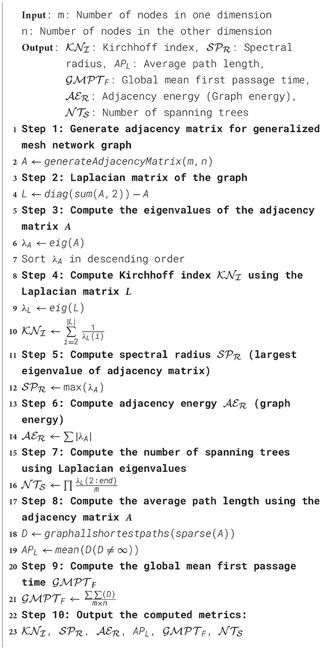
Algorithm 1. Compute metrics for the generalized mesh network.

Table 1

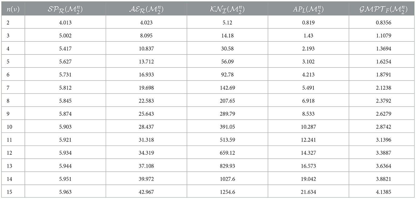
Table 1. Assessment of network-related parameters for the generalized mesh network graph $\left({\mathcal{M}}_m^n\right)$ with m set to 2, where 2 ≤ n ≤ 15.

Table 2

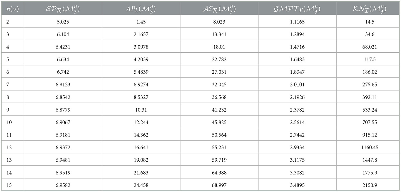
Table 2. Assessment of network-related parameters for the generalized mesh network graph $\left({\mathcal{M}}_m^n\right)$ with m set to 3, where 2 ≤ n ≤ 15.

Figure 2

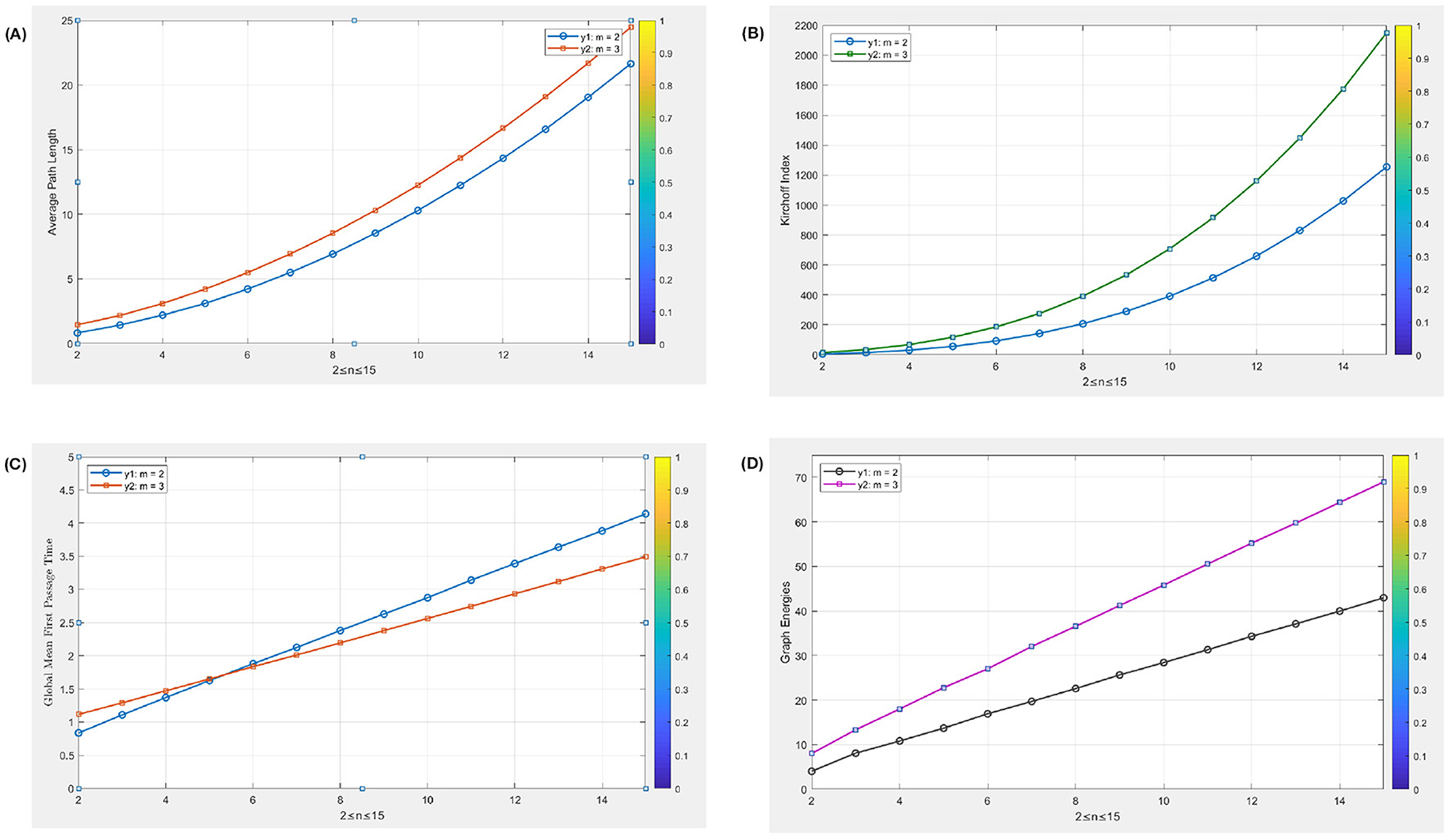
Figure 2. Comparative representation of numeric values evaluated in Tables 1 and 3 for Generalized mesh network graph $\left({\mathcal{M}}_m^n\right)$ with m set to 2, where 2 ≤ n ≤ 15. (A) Average Path Length of $\left({\mathcal{M}}_m^n\right)$. (B) Kirchoff Index of $\left({\mathcal{M}}_m^n\right)$. (C) Global passage time of $\left({\mathcal{M}}_m^n\right)$. (D) Graph energies of $\left({\mathcal{M}}_m^n\right)$.

A key observation in the graphical representations is the clear trend indicating that as the network expands, several key metrics increase significantly. These visuals enhance the understanding of the network's behavior, complementing the numerical data and offering a more intuitive grasp of the dynamics within the generalized mesh network. The graphical depiction of the results provides a glimpse into the potential of our methodologies. Researchers are encouraged to utilize our carefully developed algorithm and analysis framework to explore the complexities of more sophisticated real-world networks. The flexibility of our approach offers a valuable toolset, enabling a deeper understanding of network behavior and performance in various contexts. This work paves the way for further studies, serving as a platform for future exploration of complex networks with improved precision and efficiency Algorithm 2).

Algorithm 2

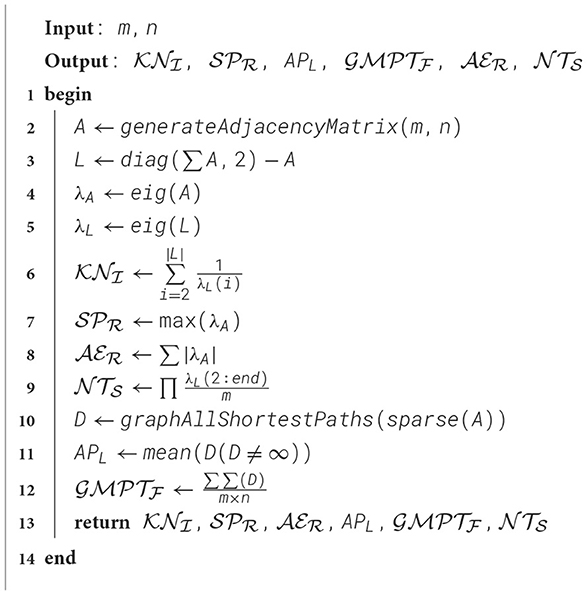
Algorithm 2. Pseudocode for computing metrics of the generalized mesh network.

Table 1 evaluates several network-related parameters for the Generalized Mesh Network Graph ${\mathcal{M}}_2^n$ across values of n from 2 to 15. The parameters included are the Spectral Radius ($\mathcal{S}{\mathcal{P}}_{\mathcal{R}}$), Average Edge Length ($\mathcal{A}{\epsilon }_{\mathcal{R}}$), Knot Number ($\mathcal{K}{\mathcal{N}}_{\mathcal{I}}$), Average Path Length ($\mathcal{A}{\mathcal{P}}_{\mathcal{L}}$), and Global Mean First Passage Time ($\mathcal{G}\mathcal{M}\mathcal{P}{\mathcal{T}}_{\mathcal{F}}$). As n increases, a notable trend is observed across these parameters. The Spectral Radius ($\mathcal{S}{\mathcal{P}}_{\mathcal{R}}$) shows a slight increase from 4.013 to 5.963, reflecting a gradual growth in the network's connectivity as more nodes are added. The Average Edge Length ($\mathcal{A}{\epsilon }_{\mathcal{R}}$) also increases consistently, indicating that as the network grows, the average distance between connected nodes becomes larger. The Knot Number ($\mathcal{K}{\mathcal{N}}_{\mathcal{I}}$), which quantifies the number of key nodes in the network, increases significantly, suggesting that more nodes are becoming central as the network expands. The Average Path Length (AP_L) increases from 0.819 to 21.634, showing that the average distance between any two nodes grows with the size of the network. Finally, the Global Mean First Passage Time ($\mathcal{G}\mathcal{M}\mathcal{P}{\mathcal{T}}_{\mathcal{F}}$) increases from 0.8356 to 4.1385, reflecting that it takes more time on average for a random walker to reach a target node as the network becomes larger. Table 1 provides similar parameters for the Generalized Mesh Network Graph ${\mathcal{M}}_3^{\mathcal{n}}$. The parameters assessed are the Spectral Radius ($\mathcal{S}{\mathcal{P}}_{\mathcal{R}}$), Average Path Length (AP_L), Average Edge Length ($\mathcal{A}{\epsilon }_{\mathcal{R}}$), Global Mean First Passage Time ($\mathcal{G}\mathcal{M}\mathcal{P}{\mathcal{T}}_{\mathcal{F}}$), and Knot Number ($\mathcal{K}{\mathcal{N}}_{\mathcal{I}}$). Trends in these parameters show a clear pattern of growth and increase with respect to the network size.

The Spectral Radius ($\mathcal{S}{\mathcal{P}}_{\mathcal{R}}$) increases from 5.025 to 6.9582, indicating a growth in the connectivity strength as the network size increases. The Average Edge Length ($\mathcal{A}{\epsilon }_{\mathcal{R}}$) increases with network size, which is consistent with the observed trend in Table 3, suggesting that longer edges become more prevalent in larger networks. The Average Path Length (AP_L) shows a notable increase from 1.45 to 24.458, similar to Table 3, indicating that as the network grows, the average distance between nodes becomes larger. The Global Mean First Passage Time ($\mathcal{G}\mathcal{M}\mathcal{P}{\mathcal{T}}_{\mathcal{F}}$) also increases from 1.1165 to 3.4895, indicating that it takes more time, on average, for a random walker to reach a target node in a larger network. The Knot Number ($\mathcal{K}{\mathcal{N}}_{\mathcal{I}}$) increases significantly from 14.5 to 2150.9, suggesting a rise in the centrality and importance of nodes within the network as its size expands. Both tables show consistent trends with increasing network size. For ${\mathcal{M}}_2^{\mathcal{n}}$, the parameters reflect a gradual increase in spectral radius, average edge length, Kirchoff Index, and average path length, leading to a higher global mean first passage time. Similarly, for ${\mathcal{M}}_3^{\mathcal{n}}$, there is a clear upward trend in the spectral radius, average edge length, average path length, and global mean first passage time, with a much more pronounced increase in the Kirchoff Index. These trends illustrate that as the network size increases, the network's complexity grows, resulting in longer paths and higher passage times. The increasing Kirchoff Index indicates more significant central nodes or hubs, which can be crucial for understanding the network's connectivity and efficiency.

Table 3

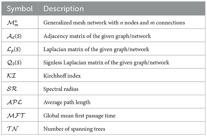
Table 3. List of symbols and their descriptions.

6 Conclusion

In summary, this article presents a comprehensive investigation into the spectral properties of the generalized mesh network graph, focusing on adjacency, Laplacian, and signless Laplacian spectra. Through advanced algebraic techniques, we have effectively analyzed these spectral characteristics to derive critical network parameters, including the Kirchhoff index ($\mathcal{K}{\mathcal{N}}_{\mathcal{I}}$), Spectral radius ($\mathcal{S}{\mathcal{P}}_{\mathcal{R}}$), Average path length (AP_L), Global mean first passage time ($\mathcal{G}\mathcal{M}\mathcal{P}{\mathcal{T}}_{\mathcal{F}}$), Graph energies ($\mathcal{A}{\epsilon }_{\mathcal{R}}$), and the number of spanning trees (${\mathcal{NT}}_{\mathcal{S}}$). Our analysis highlights the utility of Laplacian spectra in calculating and understanding various aspects of network behavior. By presenting the results in graphical form, we have provided a clear visualization of how these parameters vary with network dimensions, enhancing our understanding of their interplay and impact. This work not only deepens our insight into the structural and dynamic properties of generalized mesh networks but also offers a robust framework applicable to more complex real-world networks. The methods demonstrated here can be adapted and extended to address specific research needs, facilitating the exploration and optimization of various network configurations. The versatility and precision of these techniques underscore their potential in advancing the study of network systems and their practical applications.

Data availability statement

The original contributions presented in the study are included in the article/supplementary material, further inquiries can be directed to the corresponding author.

Author contributions

AR: Conceptualization, Visualization, Writing – original draft. MM: Software, Supervision, Writing – review & editing.

Funding

The author(s) declare that no financial support was received for the research and/or publication of this article.

Conflict of interest

The authors declare that the research was conducted in the absence of any commercial or financial relationships that could be construed as a potential conflict of interest.

Generative AI statement

The author(s) declare that Gen AI was used in the creation of this manuscript. During the preparation of this work the author(s) used AIL Models in order to improve the English writing as authors belong to non-English region. After using this tool/service, the author(s) reviewed and edited the content as needed and take(s) full responsibility for the content of the publication.

Publisher's note

All claims expressed in this article are solely those of the authors and do not necessarily represent those of their affiliated organizations, or those of the publisher, the editors and the reviewers. Any product that may be evaluated in this article, or claim that may be made by its manufacturer, is not guaranteed or endorsed by the publisher.

References

1. Merris R. Laplacian matrices of graphs: a survey. Linear Algebra Appl. (1994) 197–198:143–76. doi: 10.1016/0024-3795(94)90486-3

PubMed Abstract | Crossref Full Text | Google Scholar

2. Hong Y, Zhang XD. Sharp upper and lower bounds for largest eigenvalue of the Laplacian matrices of trees. Discrete Mathemat. (2005) 296:187–97. doi: 10.1016/j.disc.2005.04.001

Crossref Full Text | Google Scholar

3. Agaev R, Chebotarev P. On the spectra of nonsymmetric Laplacian matrices. Linear Algebra Appl. (2005) 399:157–68. doi: 10.1016/j.laa.2004.09.003

Crossref Full Text | Google Scholar

4. Rojo O, Soto R. The spectra of the adjacency matrix and Laplacian matrix for some balanced trees. Linear Algebra Appl. (2005) 403:97–117. doi: 10.1016/j.laa.2005.01.011

Crossref Full Text | Google Scholar

5. Ding X, Jiang T. Spectral distributions of adjacency and Laplacian matrices of random graphs. Ann Appl Probab. (2010) 20:2086–117. doi: 10.1214/10-AAP677

PubMed Abstract | Crossref Full Text | Google Scholar

6. Wu CW. Conditions for separability in generalized Laplacian matrices and diagonally dominant matrices as density matrices. Physics Letters A. (2006) 351:18–22. doi: 10.1016/j.physleta.2005.10.049

Crossref Full Text | Google Scholar

7. Kaveh A, Rahami H. Block diagonalization of adjacency and Laplacian matrices for graph product; applications in structural mechanics. Int J Numer Methods Eng. (2008) 68:33–63. doi: 10.1002/nme.1696

Crossref Full Text | Google Scholar

8. Spielman DA. Algorithms, graph theory, and linear equations in Laplacian matrices. In: Proceedings of the International Congress of Mathematicians (ICM 2010). New Delhi: Hindustan Book Agency (2010). p. 2698–2722.

PubMed Abstract | Google Scholar

9. Estrada E. Path Laplacian matrices: Introduction and application to the analysis of consensus in networks. Linear Algebra Appl. (2012) 436:3373–91. doi: 10.1016/j.laa.2011.11.032

Crossref Full Text | Google Scholar

10. Krishnan D, Fattal R, Szeliski R. Efficient preconditioning of Laplacian matrices for computer graphics. ACM Trans Graph. (2013) 32:1–15. doi: 10.1145/2461912.2461992

Crossref Full Text | Google Scholar

11. Dong X, Thanou D, Frossard P, Vandergheynst P. Laplacian matrix learning for smooth graph signal representation. In: 2015 IEEE International Conference on Acoustics, Speech and Signal Processing (ICASSP). Piscataway, NJ: IEEE (2015). p. 3736–3740.

PubMed Abstract | Google Scholar

12. Pirani M, Sundaram S. On the smallest eigenvalue of grounded Laplacian matrices. IEEE Trans Automat Contr. (2016) 61:509–14. doi: 10.1109/TAC.2015.2444191

Crossref Full Text | Google Scholar

13. Bergamaschi L., Martínez A. (2015). Efficiently preconditioned inexact Newton methods for large symmetric eigenvalue problems. Optimiz Methods Softw. 30:301–22. doi: 10.1080/10556788.2014.908878

Crossref Full Text | Google Scholar

14. Bandeira AS. Random Laplacian matrices and convex relaxations. Found Comput Mathem. (2018) 18:345–79. doi: 10.1007/s10208-016-9341-9

Crossref Full Text | Google Scholar

15. Zhou S, Liu X, Liu J, Guo X, Zhao Y, Zhu E, et al. Multi-view spectral clustering with optimal neighborhood laplacian matrix. In: Proceedings of the AAAI Conference on Artificial Intelligence. Palo Alto, CA: AAAI Press (2020). p. 6965–72.

Google Scholar

16. Li W. Quotient with a general orthogonality constraint and an eigen-balanced Laplacian matrix: the greatest lower bound and applications in cooperative control problems. IEEE Trans Automat Contr. (2018) 63:4024–31. doi: 10.1109/TAC.2018.2815179

Crossref Full Text | Google Scholar

17. Hermann J, Konigorski U. Eigenvalue assignment for the laplacian matrix of directed graphs. In: Proceedings of the 2019 American Control Conference (ACC). Philadelphia, PA: ACC. (2019). p. 4036–4042.

Google Scholar

18. Bergamaschi L, Bozzo E. Computing the smallest Eigenpairs of the graph Laplacian. SeMA J. (2018) 75:1–16. doi: 10.1007/s40324-017-0108-2

Crossref Full Text | Google Scholar

19. Jog SR, Kotambari R. On the adjacency, laplacian, and signless laplacian spectrum of coalescence of complete graphs. J Graph Theory. (2016) 82:5906801. doi: 10.1155/2016/5906801

Crossref Full Text | Google Scholar

20. Alhevaz A, Baghipur M, Ganie HA, Pirzada S. Brouwer type conjecture for the eigenvalues of distance signless Laplacian matrix of a graph. Linear Multilinea Algebra. (2019) 69:2423–40. doi: 10.1080/03081087.2019.1679074

Crossref Full Text | Google Scholar

21. Ganie HA, Shang Y. On the spectral radius and energy of signless Laplacian matrix of digraphs. Heliyon. (2022) 8:e09186. doi: 10.1016/j.heliyon.2022.e09186

PubMed Abstract | Crossref Full Text | Google Scholar

22. Morbidi F. Functions of the Laplacian matrix with application to distributed formation control. IEEE Trans Cont Netw Syst. (2022) 9:1459–67. doi: 10.1109/TCNS.2021.3113263

Crossref Full Text | Google Scholar

23. Reinhart C. The normalized distance Laplacian. Special Matrices. (2021) 9:1–18. doi: 10.1515/spma-2020-0114

Crossref Full Text | Google Scholar

24. Chakrabarty A, Hazra RS, Hollander F, Sfragara M. Spectra of adjacency and Laplacian matrices of inhomogeneous Erdos-Rényi random graphs. Random Matric. (2021) 10:2150009. doi: 10.1142/S201032632150009X

Crossref Full Text | Google Scholar

25. Alazemi A, Anđelić M, Koledin T, Stanic Z. Chain graphs with simple Laplacian eigenvalues and their Laplacian dynamics. Computat Appl Mathem. (2022) 42:6. doi: 10.1007/s40314-022-02141-5

Crossref Full Text | Google Scholar

26. Anđelić M, da Fonseca CM, Kilic E, Stanic Z. A Sylvester-Kac matrix type and the Laplacian controllability of half graphs. Electron J Linear Algebra. (2022) 2022:38. doi: 10.13001/ela.2022.6947

Crossref Full Text | Google Scholar

27. Bapat RB, Jana R, Pati S. The bipartite Laplacian matrix of a nonsingular tree. Special Matrices. (2023) 11:20230102. doi: 10.1515/spma-2023-0102

Crossref Full Text | Google Scholar

28. Anđelić M, Brunetti M, Stanic Z. Laplacian controllability for graphs obtained by some standard products. Graphs Combinat. (2020) 36:1593–602. doi: 10.1007/s00373-020-02212-6

Crossref Full Text | Google Scholar

29. Anđelić M, da Fonseca CM, Simić SK, Toć DV. Connected graphs of fixed order and size with maximal Q-index: some spectral bounds. Discrete Appl Mathemat. (2012) 160:448–59. doi: 10.1016/j.dam.2011.11.001

Crossref Full Text | Google Scholar

30. Mallik S. Matrix tree theorem for the net Laplacian matrix of a signed graph. Linear Multilinear Algebra. (2024) 72:1138–52. doi: 10.1080/03081087.2023.2172544

Crossref Full Text | Google Scholar

31. Raza A, Munir M, Abbas T, Eldin SM, Khan I. Spectrum of prism graph and relation with network related quantities. AIMS Math. (2023) 8:2634–47. doi: 10.3934/math.2023137

Crossref Full Text | Google Scholar

32. Raza A, Munir MM. Insights into network properties: spectrum-based analysis with Laplacian and signless Laplacian spectra. Eur Physi J Plus. (2023) 138:802. doi: 10.1140/epjp/s13360-023-04441-z

Crossref Full Text | Google Scholar

33. Raza A, Munir M, Hussain M, Tolasa FT. A spectrum-based approach to network analysis utilizing Laplacian and signless laplacian spectra to torus networks. IEEE Access. (2024) 12:52016–52029. doi: 10.1109/ACCESS.2024.3384300

Crossref Full Text | Google Scholar

34. Harel D, Sardashti A. Structural characteristics of grid graphs. J Graph Theory. (1998) 27:133–48.

Google Scholar

35. Hinz AM, Holz auf der Heide C. An efficient algorithm to determine all shortest paths in Sierpinski graphs. Discrete Appl Math. (2014) 177:111–20. doi: 10.1016/j.dam.2014.05.049

Crossref Full Text | Google Scholar

36. Yang Y, Liu H, Hou J, Zhang N, Wu T. Data collection of wireless sensor network with grid structure based on compressed sensing. In: 2021 IEEE 4th International Conference on Electronic Information and Communication Technology (ICEICT), Xi'an, China (2021) p. 363–8. doi: 10.1109/ICEICT53123.2021.9531288

Crossref Full Text | Google Scholar

37. Fang X, Misra S, Xue G, Yang D. A survey of smart grid architectures, applications, benefits and standardization. J Netw Comput Appl. (2012) 35:1950–62. doi: 10.1016/j.jnca.2012.07.002

Crossref Full Text | Google Scholar

38. Trinajstic N, Babic D, Nikolic S, Plavšic D, Amic D, Mihalic Z. The Laplacian matrix in chemistry. J Chem Inform Comput Sci. (1994) 34:368–76. doi: 10.1021/ci00018a023

Crossref Full Text | Google Scholar

39. Chu Z, Munir M, Yousaf A, Qureshi MI, Liu J. Laplacian and signless Laplacian spectra and energies of multi-step wheel networks. Mathem Biosci Eng. (2020) 17:3649–59. doi: 10.3934/mbe.2020206

PubMed Abstract | Crossref Full Text | Google Scholar

40. Xu Y, Feng Z, Qi X. Signless-Laplacian eigenvector centrality: a novel vital nodes identification method for complex networks. Pattern Recognit. Letters. (2021) 148:7–14. doi: 10.1016/j.patrec.2021.04.018

Crossref Full Text | Google Scholar

41. Pecora LM, Sorrentino F, Hagerstrom AM, Murphy TE, Roy R. How do the eigenvalues of the Laplacian matrix affect route to synchronization patterns. Phys Lett A. (2014) 378:2590–5. doi: 10.1016/j.physleta.2014.07.019

Crossref Full Text | Google Scholar

42. Mohar B. Some applications of Laplace eigenvalues of graphs. In: Hahn G, Sabidussi G, , editors. Graph Symmetry. NATO ASI Series, Vol. 497. Dordrecht: Springer (1997). doi: 10.1007/978-94-015-8937-6_6

PubMed Abstract | Crossref Full Text | Google Scholar

43. Lukovits I, Nikolić S, Trinajstić N. Resistance distance in regular graphs. Int J Quant Chem. (1999) 71:217–225.

Google Scholar

44. Szabó GJ, Alava M, Kertész J. Geometry of minimum spanning trees on scale-free networks. Physica A. (2003) 330:31–6. doi: 10.1016/j.physa.2003.08.031

Crossref Full Text | Google Scholar

45. Wu ZH, Braunstein LA, Havlin S, Stanley HE. Transport in weighted networks: partition into superhighways and roads, Phys. Rev Lett. (2006) 96:148702. doi: 10.1103/PhysRevLett.96.148702

PubMed Abstract | Crossref Full Text | Google Scholar

46. Dhar D. Theoretical studies of self-organized criticality. Physica A. (2006) 369:29–70. doi: 10.1016/j.physa.2006.04.004

Crossref Full Text | Google Scholar

47. Dhar D, Dhar A. Distribution of sizes of erased loops for loop-erased random walks, Phys. Rev E. (1997) 55:R2093. doi: 10.1103/PhysRevE.55.R2093

Crossref Full Text | Google Scholar

48. Zhang ZZ, Wu B, Comellas F. The number of spanning trees in Apollonian networks, Discrete Appl. Math. (2014) 169:206–13. doi: 10.1016/j.dam.2014.01.015

Crossref Full Text | Google Scholar

49. Godsil C, Royle G. Algebraic Graph Theory, Graduate Texts in Mathematics. New York: Springer. (2001). p. 207.

PubMed Abstract | Google Scholar

50. Liu P, Liu G, Lv H. Power function method for finding the spectral radius of weakly irreducible nonnegative tensors. Symmetry. (2022) 14:2157. doi: 10.3390/sym14102157

Crossref Full Text | Google Scholar

51. Jiang Z, Li L, Xu Y. Spectral Radius Optimization for Neural Networks. Neural Networks. (2020) 122:359–69.

Google Scholar

52. Klein DJ, Randic M. Resistance distances. J Math Chem. (1993) 12:81–95. doi: 10.1007/BF01164627

Crossref Full Text | Google Scholar

53. Li S, Zhang Q, Wang Y, Li X. Graph energies and network robustness. J Complex Netw. (2022) 1–15.

Google Scholar

54. Lee JR, Hussain A, Fahad A, Raza A, Qureshi MI, et al. On ev and ve-Degree Based Topological Indices of Silicon Carbides. CMES. (2022) 130:871–85. doi: 10.32604/cmes.2022.016836

Crossref Full Text | Google Scholar

55. Fowler PW. Energies of graphs and molecules. AIP Conf Proc. (2007) 963:517–20. doi: 10.1063/1.2836127

Crossref Full Text | Google Scholar

56. Zhang X, Raza A, Fahad A, Jamil MK. (2020). On face index of silicon carbides. Discrete Dyn Nat Soc. 2020:6048438. doi: 10.1155/2020/6048438

PubMed Abstract | Crossref Full Text | Google Scholar

57. Truong QD, Truong QB, Dkaki T. Graph methods for social network analysis. In: Vinh P, Barolli L, , editors. Nature of Computation and Communication. ICTCC 2016. Lecture Notes of the Institute for Computer Sciences, Social Informatics and Telecommunications Engineering, Vol. 168. Cham: Springer (2016). doi: 10.1007/978-3-319-46909-6_25

Crossref Full Text | Google Scholar

58. Alghazzawi D, Raza A, Munir U, Ali S. Chemical applicability of newly introduced topological invariants and their relation with polycyclic compounds. J Mathemat. (2022) 2022:5867040. doi: 10.1155/2022/5867040

Crossref Full Text | Google Scholar

59. Ramana KVM, Shireesha R. Applications of spectral graph theory in machine learning and data science. Global J Eng Innov Interdiscipl Res. (2025) 5:1–6. doi: 10.33425/3066-1226.1070

Crossref Full Text | Google Scholar

60. Morzy M, Kajdanowicz T. Graph energies of egocentric networks and their correlation with vertex centrality measures. Entropy. (2018) 20:916. doi: 10.3390/e20120916

PubMed Abstract | Crossref Full Text | Google Scholar

61. Chen D, Nie M, Wang J, Kong Y, Wang D, Huang X. Community detection based on graph representation learning in evolutionary networks. Appl Sci. (2021) 11:4497. doi: 10.3390/app11104497

Crossref Full Text | Google Scholar