A new tool to detect financial data scaling

The assumption of frictionless markets has long been debated, drawing interest from scholars and practitioners alike. Market liquidity is a central theme in this regard; it is traditionally assessed through transaction costs, volume, price-based, and market-impact measures. In contrast, the Fractal Market Hypothesis (FMH) suggests that liquidity emerges from the heterogeneity of investment time scales among participants, with liquidity shortages arise when traders converge on the same time horizons, particularly the short-term one which typically occurs during volatile periods. While current methods to asses liquidity often rely on single moments, which may provide limited insights, a novel methodology that considers the whole distributions and compares log-returns across pairs of time scales is discussed and implemented in this work. A Matlab-based algorithm is built that provides as output a dynamical estimation of the pairwise self-similarity of the scaled distributions. The lower the self-similarity parameter the higher the potential liquidity shortage.

1 Introduction

The assumption of frictionless markets has been a longstanding topic of debate, attracting interest from both scholars and market practitioners. Broadly speaking, financial market frictions encompass any factors that impede natural trading and may include transaction costs, taxes, regulatory expenses, asset indivisibility, and liquidity constraints. Notably, the concept of market liquidity is a cornerstone in financial literature, with traditional liquidity measures generally categorized into four groups [1]: (a) transaction cost measures, such as the bid-ask spread and its extensions [2]; (b) volume-based measures, including transaction volume, turnover [3], and the Hui–Heubel Liquidity Ratio [4]; (c) price-based measures, for instance, the Amihud measure (ILLIQ) [5] and the Market Efficiency Coefficient (MEC) [6]; (d) market-impact measures, exemplified by the Market-Adjusted Liquidity Model developed by Hui and Heubel in 1984 [4].

The introduction of electronic trading systems in recent years have increased the attention toward another measure of liquidity: the order book. It captures the orders placed by traders to buy and sell stocks at different price points. In this direction, a very interesting work by Libman et al. [7] concludes that the deeper layers of the order book possess valuable information in the context of liquidity, a finding that is supported by other studies.

A radically different approach to modeling market liquidity is proposed by the Fractal Market Hypothesis (FMH) [8]. This posits that liquidity is driven by the heterogeneity of investment time horizons among market participants. Under normal conditions, investors operate on a variety of time horizons, from intraday (fractions of seconds or minutes) to several years (pension funds, institutional investors); liquidity originates from the different expectations (and probability assessments) of market participants looking at different time-scaled distributions of financial returns. Therefore, a lack of liquidity can occur when the distributions among time scales appear similar or when trading activity ceases on some relevant time scales and investors start trading on common (typically short-term) horizons. In these cases, usually occurring during periods of high volatility where rising uncertainty results in a shift toward quick buy-and-sell operations, trading can slow or even be freezed, simply because most of traders—who are supposedly rational—base their trading decisions on similar distributions which induce similar behaviors. Typically, short-term investors rely more heavily on technical information, whereas long-term investors focus on fundamental indicators [9]. In the event of a significant market crash that challenges fundamental assumptions, long-term investors may either exit the market or shift to short-term strategies [10]. The Fractal Market Hypothesis can also be used to assess the causes of financial (in)stability, as suggested by Anderson and Noss [11]. In particular, the analysis reveals some relevant implications to a number of ongoing debates regarding the regulation of financial markets and of their major participants. A review of the Fractal Market Hypothesis together with the basic principles of fractal geometry is provided by Blackledge and Lamphiere [12]. Specifically, they consider the intrinsic scaling properties that characterize a random walk and the Efficient Market Hypotheses and exploring the Lévy index, coupled with other metrics, such as the Lyapunov exponent and the volatility, a long-term forecasts analysis is developed. In a study of two developed market indices and one emerging market index, Karp and Van Vuuren [13] find a relationship between the change in a time series' fractal dimension (before breaching a threshold) and both the magnitude and direction of the subsequent change in the time series. This relationship was found to be prevalent during times of strong price persistence, characterized by elevated Hurst exponents, suggesting potential investment strategies.

From a mathematical perspective, while various methods—such as DFA, wavelet power spectra, variance scaling, and R/S analysis—have been proposed to quantify liquidity in terms of scale invariance (see [14] or [15] for a comprehensive discussion), most traditional approaches primarily examine single moments rather than full distributions, which may yield incomplete insights. The aim of this work is to present the implementation of a novel methodology that examines self-similarity and (il)liquidity by comparing the entire distributions of log-returns over pairs of time scales, rather than only specific moments. In particular, an algorithm and a ready-to-use Matlab software are discussed to evaluate liquidity through the analysis of a time indexed self-similarity matrix whose entries are the pairwise self-similarity parameters relating the log-returns distributions across different investment time horizons (from 1 day up to 6 months). Roughly speaking, the estimated parameters tell how diverse the paired distributions are.

The methodology we implement provides insights into both market liquidity and the evolution of return distributions across time scales. Thus, it can provide insights to market makers and regulators particularly during periods of market turbulence. Indeed, the 2007–2009 global financial crisis, as well as the recent pandemic and geopolitical crises, have underscored the importance of understanding liquidity and its underlying drivers in financial markets.

The remainder of this article is organized as follows: Section 2 outlines the theoretical framework and the self-similarity testing procedure employed in this study. Section 3 presents the proposed algorithm, and Section 4 concludes.

2 Theoretical background and methodology

In subSection 2.1 the definition of self-similarity is introduced along with the justification of its usage in financial context. SubSection 2.2 shortly discusses how self-similarity can be evaluated using the Kolmogorov–Smirnov distribution. Both topics are introduced to clarify how the methodology has been implemented in the software introduced in Section 3.

2.1 Self-similarity

Definition 2.1. [16] A stochastic process {X_t, t ≥ 0} in ℝ^k, continuous at t = 0, is self-similar with parameter H₀ ≥ 0 (denoted H₀-ss) if, for all scaling factors a > 0, the following holds:

$\begin{array}{ll}\{X_{at}\}\stackrel{d}{=}\{a^{H_0}{X}_t\},& (1)\end{array}$

where $\stackrel{d}{=}$ denotes that the finite-dimensional distributions of {X_at} and $\{a^{H_0}{X}_t\}$ are equal.

Remark 2.1. The process is trivial (H = 0) if and only if X_t = X₀ almost surely for all t > 0. Additionally, if 𝔼(|X₁|) < ∞, then H ≤ 1 [17], meaning non-degenerate processes have H ∈ (0, 1]. A common example is Brownian motion, which is $\frac{1}{2}$-self-similar.

Consider now a H₀-self-similar process {X(t)} with stationary increments, and let Y(t, a) = X(t + a) − X(t) denote the increments over lag a. Due to stationarity, $\left\{Y(t,a)\right\}\stackrel{d}{=}\{Y(T,a)\}$ for any times t and T. It is easy to check that Y(t, a) is also self-similar with the same parameter H₀, i.e. that

$\begin{array}{ll}\{Y(t,a)\}\stackrel{d}{=}\{a^{H_0}Y(t,1)\},& (2)\end{array}$

and X_t is said H₀-sssi (self-similar of parameter H₀ with stationary increments).

Remark 2.2. In financial applications, let X_t = ln P_t, where P_t is the price of an asset at time t. If X_t is (at least locally) self-similar and with stationary increments, the a-lagged log-price change scales as $a^{H_0}$ times the one-lag change. This observation forms the theoretical basis for the widely-used practice of annualizing volatility in finance. Specifically, from self-similarity, we have $𝔼[X_t^2]=t^{2H_0}𝔼[X_1^2]$, and assuming 𝔼[X_t] ≈ 0, it follows that ${\sigma }_t^2\approx t^{2H_0}{\sigma }_1^2$. For volatility, this implies ${\sigma }_t\approx t^{H_0}{\sigma }_1$. Under the assumption of Brownian motion (with H₀ = 1/2), this simplifies to the familiar relation ${\sigma }_t\approx \sqrt{t}{\sigma }_1$, which is commonly used by practitioners to scale volatility over different time horizons.

In this regard, the methodology is particularly well-suited to classes of financial instruments that are continuously traded in financial markets and exhibit a certain degree of risk (including commodities or cryptocurrencies), while it proves less applicable to instruments with a low level of risk, such as, for example, the fixed income.

2.2 Testing for Self-Similarity

To estimate the self-similarity parameter H₀, one needs to test the equality in Equations 1, or 2. To this aim, the tool which will be described in next sections follows the methodology proposed in [18–20] focusing on the increment process {Y(t, a)} for simplicity.

Let $\mathcal{A}$ be a compact set of time scales, and define $\underset{\_}{a}=min(\mathcal{A})$ and $\overline{a}=max(\mathcal{A})$, with $\underset{\_}{a}<\overline{a}$. For each $a\in \mathcal{A}$, let F_Y(a)(x) denote the cumulative distribution function (CDF) of Y(t, a). For any $a,b\in \mathcal{A}$, the self-similarity condition from Equation 2 can be rewritten as:

$\begin{array}{ll}{F}_{a^{-H_0}Y(a)}(x)=F_{b^{-H_0}Y(b)}(x).& (3)\end{array}$

Let H be a candidate parameter. From Equation 3, it follows that:

$\begin{array}{ll}{F}_{{(a/b)}^{-H}Y(a)}(x)=F_{Y(b)}\left({\left(a/b\right)}^{H-H_0}x\right).& (4)\end{array}$

We now define the set ${\text{Ψ}}_H:=\{F_{a^{-H}Y(a)}(x)\}$ and introduce a distance function ρ based on the sup-norm ||·||_∞ over the set $\mathcal{A}$. The metric space (Ψ_H, ρ) has a diameter given by:

$\begin{array}{l}\delta ({\text{Ψ}}_H)={\displaystyle \underset{x\in ℝ}{sup}}{\displaystyle \underset{a,b\in \mathcal{A}}{sup}}{\displaystyle |F_{a^{-H}Y(a)}(x)-F_{b^{-H}Y(b)}(x)|}\\ {\displaystyle ={\displaystyle \underset{x\in ℝ}{sup}}|F_{{\underset{\_}{a}}^{H-H_0}Y(1)}(x)-F_{{\overline{a}}^{H-H_0}Y(1)}(x)|.}& (5)\end{array}$

The diameter δ(Ψ_H) is minimized when H = H₀, as it decreases for H ≤ H₀ and increases for H ≥ H₀ (see [18] for the proofs). Thus, we can estimate the self-similarity parameter as:

$\begin{array}{ll}{\widehat{H}}_0=arg{\displaystyle \underset{H\in (0,1]}{min}}\widehat{\delta }({\text{Ψ}}_H),& (6)\end{array}$

where $\widehat{\delta }({\text{Ψ}}_H)$ is the empirical counterpart of δ(Ψ_H), computed using the empirical cumulative distribution function $\widehat{F}$.

Remark 2.3. Notice that the last line of Equation 5 is the two-sample Kolmogorov–Smirnov (KS) statistic, which provides the distribution of the maximum of the absolute differences between two empirical CDF, under the null hypothesis that both are drawn from the same population distribution. In particular, the goodness-of-fit of the empirical distribution can be evaluated with respect to a theoretical distribution F (Kolmogorov, D_n) or between two empirical distributions (Smirnov, (D_{n, m})) of n and m observations:

$\begin{array}{ll}{D}_{n,m}={\displaystyle \underset{x}{sup}}|F_{1,n}(x)-F_{2,m}(x)|,& (7)\end{array}$

where F_1,n and F_2,m are the empirical cumulative distribution functions of two independent samples. The statistics is non parametric and for large samples, the null hypothesis is rejected at level α if

$\begin{array}{ll}{D}_{n,m}>K_{\alpha }=\sqrt{-log(\alpha /2)\frac{1+\frac{m}{n}}{2m}}& (8)\end{array}$

When applied to the estimation of the self-similarity parameter H₀ of a sample of size n, Equation 7 becomes

$\begin{array}{ll}\widehat{\delta }({\text{Ψ}}_H)={\displaystyle \underset{x\in ℝ}{sup}}{\displaystyle |\frac{1}{n-\underset{\_}{a}}{\displaystyle \sum _{i=1}^{n-\underset{\_}{a}}}{1}_{X_{1,i}\le {\underset{\_}{a}}^{H}x}-\frac{1}{n-\overline{a}}{\displaystyle \sum _{i=1}^{n-\overline{a}}}{1}_{X_{1,i}\le {\overline{a}}^{H}x}|}& (9)\end{array}$

The distribution (Equation 8) of the KS statistic is well-known when the samples are independent, i.e. when H₀ = 1/2. For values of H₀ > 1/2, the process exhibits positive autocorrelation increasing with the distance from 1/2 and decreasing with the lag at such a slow rate that the autocorrelation function becomes non-summable (the so-called long-term memory). For H < 1/2, the process displays short-term memory characterized by negative autocorrelation. These positive and negative autocorrelations result in a Type I error for H > 1/2 and a Type II error for H < 1/2, i.e. the KS critical value tends to be too restrictive for moderate to high levels of positive autocorrelation and too lenient for moderate to high levels of negative autocorrelation. Since in these cases the distribution of the test statistic is not explicitly known and it is also difficult to be derived analytically, we have implemented Monte Carlo simulations to deduce the p-values for different values of H₀. The results are summarized in Table 1.

Table 1

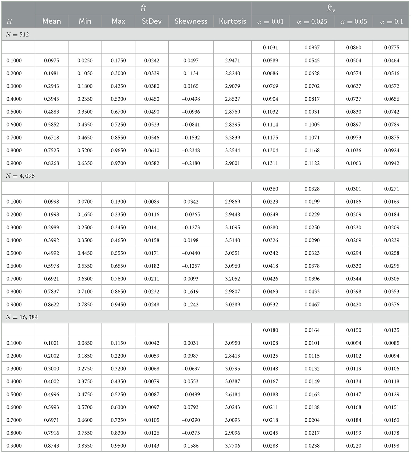
Table 1. Estimates of H and K_α and summary statistics.

Given the daily distribution of returns of the all stocks forming a stock index, the value Ĥ₀ of Equation 11 can be calculated at any time t and any pair of time scales a, b in the set $\mathcal{A}=\{1,2,\dots ,N\}$. Thus, a symmetric self-similarity matrix can be built as

$\begin{array}{ll}\widehat{\text{H}}(\text{t})=\left[\widehat{H}(a,b,t)\right]& (10)\end{array}$

with

$\begin{array}{ll}\widehat{H}(a,b,t)=arg{\displaystyle \underset{H\in (0,1]}{min}}\left({\displaystyle \underset{x\in ℝ}{max}}{\displaystyle |{\widehat{F}}_{Y(t,a)}(x)-{\widehat{F}}_{Y(t,b)}\left({\left(b/a\right)}^{H}x\right)|}\right).& (11)\end{array}$

Of course, since Ĥ₀(a, b, t) = Ĥ₀(b, a, t) the resulting estimation will consist in a time-indexed sequence of lower (upper) triangular matrices.

3 Algorithm for testing self-similarity

The pseudocode Algorithm 1 provides a structured overview of the function SelfSimilarity, detailing the nested loop structure, the determination of rescaled sequences, and the two-sample Kolmogorov–Smirnov (KS) test implementation.

Algorithm 1

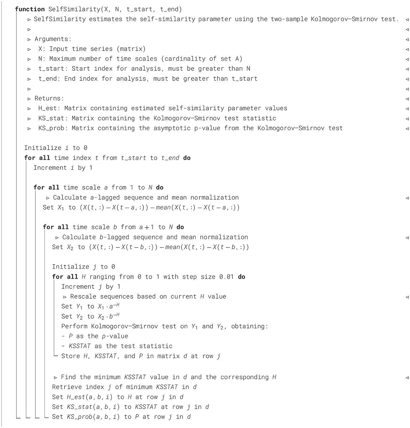
Algorithm 1. Estimation of the self-similarity parameter.

In detail, the algorithm iteratively estimates self-similarity on different time scales and intervals, aiming to find the parameter H that minimizes the KS statistic, thereby quantifying the self-similarity index between two paired lagged sequences. The function receives four input values: the time sequence X(t, m) (log-price for financial applications), which stores m paths of length t; the maximum number of time scales N and the indices of the startpoint and endpoint of the analysis. Within nested loops that iterate over time indices, time scales and a range of potential H values, the algorithm generates lagged sequences for each pair of scales and performs the KS test to assess distributional similarity. The KS statistic and its associated p-value are stored, enabling the identification of the optimal H for each pair of scales. Finally, the function outputs matrices containing the estimated self-similarity parameter, the KS statistic, and the p-value across all analyzed time scales and indices, providing a robust measure of self-similarity in the time series data.

Regarding the two-sample Kolmogorov–Smirnov test used by the algorithm, it should be noted that this test is readily available in the standard function libraries of most major programming languages. Implementations in languages such as Python, MATLAB, and R provide accessible and optimized functions that allow users to efficiently perform the KS test to assess whether two samples come from the same distribution. These library functions typically offer flexibility in terms of input parameters, enabling control over test options such as significance levels and alternative hypotheses.

To demonstrate the effectiveness of the proposed algorithm with real data, it was implemented in the MATLAB R2024a environment and tested on a computer with a 64-bit Windows operating system, an Intel Core i7-10510U CPU (1.80 GHz–2.30 GHz), and 16 GB of RAM. The input matrix X was constructed using the logarithmic prices of 183 assets continuously listed in the S&P500 index (Standard and Poor's, USA) from January 2000 to December 2023, totaling 6,037 observations. Even if 183 out of 500 individual stocks were consider as representative of the index, constructing the distribution from the all stocks that make up the market index makes it possible to eliminate the inertial effect that would be observed if—instead of the individual stocks—only the time-marginal distribution of the index were considered.

The average execution time for each iteration was ~30 s.

Figure 1 illustrates three contrasting market conditions in terms of liquidity: the top row represents a period of near-total liquidity shortage, revealed by the self-similarity surface (left-hand plot) and the rescaled log-return densities, reported for the pair a = 58 and b = 72 (right-hand plot) on March 16, 2020. The self-similarity surface, dominated by a uniform blue color across all investment pairs, indicates very low values of the self-similarity parameter, signifying an extremely low liquidity level in the market due to the fact that the distributions almost overlap as they are, the scaling exponent being close to zero. This outcome aligns with expectations, as this date was chosen during the U.S. quarantine or lockdown period, where markets were affected by heightened concerns regarding the COVID-19 pandemic's progression. Additional evidence appears in the right panel, where both rescaled densities exhibit a pronounced left-skewed tail.

Figure 1

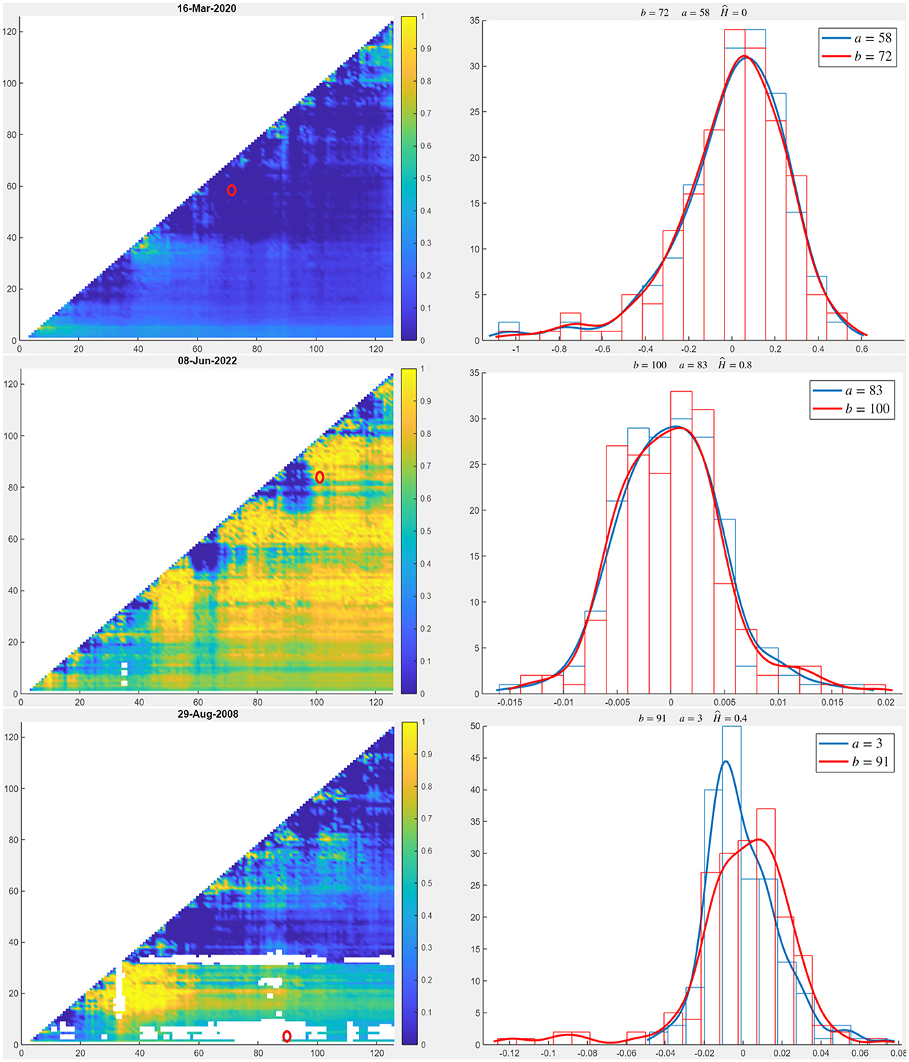
Figure 1. Self-similarity matrices $\widehat{\text{H}}(\text{t})$ sampled at days March 16, 2020 (top-left), June 08, 2022 (middle-left) and August 29, 2008 (bottom-left) and corresponding rescaled densities of log-returns for the pair a = 58, b = 72 (top-right), a = 83, b = 100 (middle-right) and a = 3, b = 91 (bottom-right). The colormap indicates the value H₀ ∈ (0, 1]. Being the matrices symmetric, to ease visualization only the associated triangular matrices are displayed in the plots.

In contrast, the plots in the mid row illustrate market liquidity conditions on June 8, 2022, when the S&P index rose by 1% or 39.25 points, with positive performance across most sectors. The self-similarity surface (left-hand plot) displays high values (yellow shading) for nearly all the considered investment pairs, indicating a high-liquidity market. In the corresponding right-hand plot, the rescaled log-return densities for the pair a = 83 and b = 100 are shown, featuring right-skewed tails. Finally, the plots in the bottom row illustrate a scenario in which self-similarity is rejected at a 95% significance level on August 29, 2008. In this case, “holes" appear in the similarity surface (blank areas), as the two densities (right-hand plot) are significantly different. At H = 0.4, the distance between the distributions is minimized but remains statistically significant; therefore, self-similarity is rejected (i.e., no value of the parameter H satisfies the distributional equality for the pair a = 3 and b = 91).

Figure 2 illustrates two summary measures for the daily distributions of Ĥ(t) and the estimated diameters $\widehat{\delta }({\text{Ψ}}_{\widehat{H}(t)})$. To improve the readability of the graphs, the entire dataset was downsampled using a 20-day step, corresponding to an average trading month. The median value and the InterQuartile Range (IQR = P₇₅(·) − P₂₅(·)) were then computed for the distributions of both Ĥ(t) and $\widehat{\delta }({\text{Ψ}}_{\widehat{H}(t)})$. The data are particularly interesting because the dynamics of P₅₀Ĥ(t) are fully consistent with the known estimates of the Hurst parameter reported in the literature (see, e.g. [21–24]). Furthermore, the fact that the values oscillate around 1/2 is of particular financial significance, as this is the only value consistent with the absence of arbitrage opportunities in the market—a sort of benchmark to which the market always returns after deviations that can be more or less prolonged depending on the shocks it experiences.

Figure 2

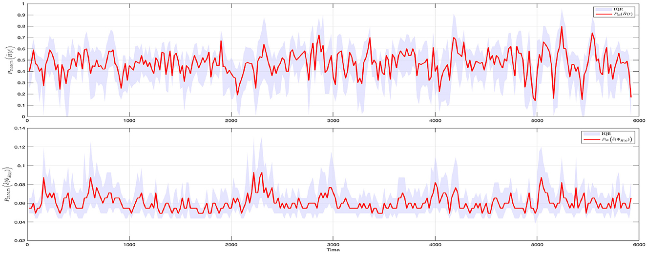
Figure 2. Interquartile range (Q3–Q1) (gray area) and median value (red line) of Ĥ(t) (top panel) and $\widehat{\delta }({\text{Ψ}}_{\widehat{H}(t)})$ (bottom panel). The plots describe the temporal evolution of two summary values of the self-similarity matrices. To ease the readability of the graphs, the dataset was downsampled with a 20-day step, corresponding to the average trading month.

4 Conclusions

In this paper, we have implemented a new methodology for assessing market liquidity. Starting from the Fractal Market Hypothesis's (FMH) assumption that liquidity emerges from the heterogeneity of investment time scales, the scale invariance or self-similarity between pairs of investment horizons is examined with regard to the whole distribution rather than, as usual, its individual moments. Specifically, the self-similarity exponent is obtained as the unknown argument that minimizes the diameter of the space of rescaled distributions, which is observed to reduce to the Kolmogorov–Smirnov statistic. A numerical procedure is built to determine this value with respect to a number of time scales flowing through time and an algorithm provides as output a dynamical estimation of the pairwise self-similarity parameter of the considered scaled distributions. Implemented in MatLab, the algorithm uses nested cycles that, for each trading day, iterates over both time scales and a range of potential values of H, and performs the KS test to assess distributional similarity. The KS statistic and its associated value are stored, allowing the optimal H for each pair of scales to be identified. Low values of the self-similarity parameter, typically occurring during volatile periods where long-term investors may either exit the market or shift to short-term scales, indicate potential liquidity shortage. In contrast, high values of the self-similarity parameter describe liquid market phases in which each time horizon is populated by a sufficient share of market participants to match trades. Empirical evidence that proves the effectiveness of the proposed algorithm with real data is offered by analyzing 183 assets continuously listed in the in the S&P500 index (Standard and Poor's, USA) from January 2000 to December 2023.

Data availability statement

The datasets presented in this article are not readily available. Requests to access the datasets should be directed to Massimiliano Frezza, bWFzc2ltaWxpYW5vLmZyZXp6YUB1bmlyb21hMS5pdA==.

Author contributions

SB: Conceptualization, Formal analysis, Supervision, Writing – review & editing. AP: Data curation, Methodology, Software, Writing – original draft. MF: Data curation, Formal analysis, Methodology, Writing – original draft. DA: Investigation, Validation, Writing – review & editing.

Funding

The author(s) declare that no financial support was received for the research, authorship, and/or publication of this article.

Conflict of interest

The authors declare that the research was conducted in the absence of any commercial or financial relationships that could be construed as a potential conflict of interest.

The author(s) declared that they were an editorial board member of Frontiers, at the time of submission. This had no impact on the peer review process and the final decision.

Generative AI statement

The author(s) declare that no Gen AI was used in the creation of this manuscript.

Publisher's note

All claims expressed in this article are solely those of the authors and do not necessarily represent those of their affiliated organizations, or those of the publisher, the editors and the reviewers. Any product that may be evaluated in this article, or claim that may be made by its manufacturer, is not guaranteed or endorsed by the publisher.

References

1. Bianchi S, Frezza M. Liquidity, Efficiency and the 2007 − 2008 global financial crisis. Ann Econ Finance. (2018) 19:375–404.

Google Scholar

2. Amihud Y, Mendelson H. Asset pricing and the bid-ask spread. J Financ Econ. (1986) 17:223–49. doi: 10.1016/0304-405X(86)90065-6

Crossref Full Text | Google Scholar

3. Dennis P, Strickland D. The effect of stock splits on liquidity and excess returns: evidence from shareholder ownership composition. J Financ Res. (2003) 26:355–70. doi: 10.1111/1475-6803.00063

Crossref Full Text | Google Scholar

4. Hui B, Heubel B. Comparative Liquidity Advantages among Major U.S. Stock Markets. Working Paper, DRI Financial Information Group Study Series, No. 84081. (1984).

Google Scholar

5. Amihud Y. Illiquidity and stock returns: cross-section and time-series effects. J Financ Mark. (2002) 5:31–56. doi: 10.1016/S1386-4181(01)00024-6

Crossref Full Text | Google Scholar

6. Hasbrouck J, Schwartz RA. Liquidity and execution costs in equity markets. J Portfolio Manag. (1988) 14:10–6. doi: 10.3905/jpm.1988.409160

Crossref Full Text | Google Scholar

7. Libman D, Haber S, Schaps M. Forecasting quoted depth with the limit order book. Front Artif Intell. (2021) 4:667780. doi: 10.3389/frai.2021.667780

PubMed Abstract | Crossref Full Text | Google Scholar

8. Peters E. Fractal Market Analysis — Applying Chaos Theory to Investment and Analysis. Hoboken, NJ: Wiley (1994).

PubMed Abstract | Google Scholar

9. Kristoufek L. Fractal markets hypothesis and the global financial crisis: scaling, investment horizons and liquidity. Adv Complex Syst. (2012) 15:1250065. doi: 10.1142/S0219525912500658

PubMed Abstract | Crossref Full Text | Google Scholar

10. Li DY, Nishimura Y, Men M. Fractal markets: liquidity and investors on different time horizons. Phys A: Stat Mech Appl. (2014) 407:144–51. doi: 10.1016/j.physa.2014.03.073

Crossref Full Text | Google Scholar

11. Anderson N, Noss J. The Fractal Market Hypothesis and its implications for the stability of financial markets. Bank of England, Financial Stability Paper n23. (2013).

Google Scholar

12. Blackledge J, Lamphiere M. A review of the fractal market hypothesis for trading and market price prediction. Mathematics. (2022) 10:117. doi: 10.3390/math10010117

Crossref Full Text | Google Scholar

13. Karp A, Van Vuuren G. Investment implications of the fractal market. Hypothesis. Ann Financ Econ. (2019) 14:1950001. doi: 10.1142/S2010495219500015

Crossref Full Text | Google Scholar

14. Mandelbrot BB. Fractals and scaling in finance. Discontinuity, Concentration, Risk Selecta Volume E. Cham: Springer (1997). doi: 10.1007/978-1-4757-2763-0

Crossref Full Text | Google Scholar

15. Cont R, Potters M, Bouchaud JP. Scaling in stock market data: stable laws and beyond. In:Dubrulle B, Graner F, Sornette D, , editors. Scale Invariance and Beyond. Berlin, Heidelberg: Springer Berlin Heidelberg (1997), p. 75–85. doi: 10.1007/978-3-662-09799-1_5

Crossref Full Text | Google Scholar

16. Lamperti J. Semi-stable stochastic process. Trans Am Math Soc. (1962) 104:62–78. doi: 10.1090/S0002-9947-1962-0138128-7

PubMed Abstract | Crossref Full Text | Google Scholar

17. Embrechts P, Maejima M. Selfsimilar Processes. Princeton, NJ: Princeton University Press (2002).

Google Scholar

18. Bianchi S. A new distribution-based test of self-similarity. Fractals. (2004) 12:331–46. doi: 10.1142/S0218348X04002586

Crossref Full Text | Google Scholar

19. Bianchi S, Pianese A, Frezza M. A distribution-based method to gauge market liquidity through scale invariance between investment horizons. Appl Stochastic Models Bus Ind. (2020) 36:809–24. doi: 10.1002/asmb.2531

Crossref Full Text | Google Scholar

20. Bianchi S, Bruni V, Frezza M, Marconi S, Pianese A, Vantaggi B, et al. An information theory approach to stock market liquidity. Chaos. (2024) 34:061102. doi: 10.1063/5.0213429

PubMed Abstract | Crossref Full Text | Google Scholar

21. Cajueiro DO, Tabak BM. The Hurst exponent over time: testing the assertion that emerging markets are becoming more efficient. Phys A Stat Mech Appl. (2004) 336:521–37. doi: 10.1016/j.physa.2003.12.031

Crossref Full Text | Google Scholar

22. Bianchi S, Pantanella A. Pointwise regularity exponents and well-behaved residuals in stock markets. Int J Trade Econ Finance. (2011) 2:52–60. doi: 10.7763/IJTEF.2011.V2.78

Crossref Full Text | Google Scholar

23. Frezza M. Modeling the time-changing dependence in stock markets. Chaos Solitons Fractals. (2012) 45:1510–20. doi: 10.1016/j.chaos.2012.08.009

Crossref Full Text | Google Scholar

24. Bianchi S, Pantanella A, Pianese A. Modeling stock prices by multifractional Brownian motion: an improved estimation of the pointwise regularity. Quant Finance. (2013) 13:1317–30. doi: 10.1080/14697688.2011.594080

Crossref Full Text | Google Scholar