A novel exponentially fitted finite-difference method for time-fractional singularly perturbed convection–diffusion problems with variable coefficients

This study presents an exponentially fitted finite-difference scheme for addressing singularly perturbed convection–diffusion problems involving the time-fractional derivative. The Caputo fractional derivative defines the time-fractional derivative. Then, the implicit finite-difference method is used to discretize the temporal variable in a uniform mesh discretization. To manage the effect of the perturbation parameter on the solution profile, an exponentially fitted factor is introduced into the resulting system of ordinary differential equations. Finally, on a uniform spatial domain discretization, an exponentially fitted scheme is developed using the Numerov finite-difference approach. The ε-uniform of the proposed scheme is rigorously demonstrated, confirming that it is uniformly convergent with a convergence order of O((Δt)^2−α+M⁻¹). The validity of the proposed method is illustrated through model examples. The numerical results match the theoretical predictions and demonstrate that the proposed method is more accurate than some recent existing methods.

1 Introduction

In numerous physical and biological systems, differential equations with parameters are commonly used to model specific behaviors or phenomena. These parameters frequently represent physical quantities such as reaction rates, diffusion coefficients, and other factors influencing solution evolution. A singularly perturbed differential equation is a differential equation in which the highest-order derivative is scaled by a small positive parameter ε. This small positive parameter, satisfying 0 ≤ ε ≪ 1, is known as the perturbation parameter. The behavior of the solution of such differential equations can vary significantly based on the values of these parameters, often resulting in intriguing and complex dynamics [1, 2]. In other words, certain thin layers, or regions within the domain experience rapid or sudden changes in the solution, forming boundary layers, whereas in regions farther from these layers, the solution remains smooth or changes more gradually.

Due to this multifarious nature of the solution, basic numerical methods like the finite-difference method, finite element method, and collocation methods often fail to effectively solve these problems, particularly as ε approaches zero [1]. To overcome these challenges, researchers were driven to develop numerical methods whose accuracy and convergence were unaffected by the influence of ε. For example, a few recent advancements in numerical methods include the higher-order uniformly convergent scheme in Anilay et al. [1], a novel numerical approach based on the exponentially adjusted operator finite-difference method in Woldaregay et al. [2], the fitted computational method in Tesfaye et al. [3], the fitted numerical scheme in Woldaregay et al. [4], and the uniformly convergent computational method in Wondimu et al. [5].

In recent decades, the theory and numerical methods of fractional calculus have attracted significant interest because differential equations of arbitrary order are often more applicable than their integer-order counterparts [6, 7]. The desire to explore the implications of extending the concept of integer order calculus to non-integer or fractional order led to the development of fractional calculus. This seemingly straightforward question gave rise to a profound and significant area of mathematical theory, finding applications across diverse fields such as physics, mathematical biology, fractal media, electromagnetics, statistical mechanics, viscoelasticity, rheology, fluid dynamics, electro-analytical chemistry, control theory, and modeling of neurons neurons, among others [8–10]. Although fractional calculus is as long as its classical calculus, it was not widely used in life problems for a long time, and it remains rarely included in modern curricula [11]. It was Oldham and Spanier [12] who published the first book dedicated exclusively to fractional calculus in 1974. Subsequently, other authors, like Podlubny [13], Miller and Roos [11], and Kilbas et al. [14], published various books on this area.

The generalization of an integer-order partial differential equation by replacing the classical-order time derivative with a fractional-order time derivative is called a time-fractional partial differential equation [8]. The analytical solutions to many of these equations are not readily available due to the challenges involved in solving these equations exactly. Even when an analytical solution exists, its construction often involves special functions, making the computations quite complex. For this reason, numerical techniques have attracted significant attention for solving such equations computationally. For instance, a second-order numerical scheme combining Crank-Nicholson and spline functions with a tension factor in Choudhary et al. [15], cubic B−spline collocation method in Choudhary et al. [16], the finite-difference scheme tailored on the Crank-Nicholson technique in Karatay et al. [17], a numerical technique using B−splines in Roul et al. [18], a cubic trigonometric spline collocation method in Yaseen et al. [19], an extended cubic B−splines in Mohyud-Din et al. [20], a computational method in Rihan [21], a higher-order collocation method in Roul and Goura [22], and a finite-difference approach based on non-uniform discretization in Fazio et al. [23] are among the recently developed numerical approaches.

A time-fractional partial-differential equation in which the highest derivative term is multiplied by a small positive parameter ε is referred to as a time-fractional singularly perturbed partial-differential equation. The small parameter ε, which multiplies the highest-order derivative term, is known as the perturbation parameter and satisfies 0 < ε ≪ 1. These equations form the central focus of this paper. Specifically, we considered the following time-fractional, singularly perturbed, partial-differential equation of the form:

$\begin{array}{ll}\{\begin{array}{l}(D_t^{\alpha }+L_{\epsilon })u(s,t)=g(s,t),\hfill \\ \forall (s,t)\in D={\text{Ω}}_s\times {\text{Ω}}_t=(0,1)\times (0,T],\hfill \\ u(0,t)={\psi }_l(t),u(1,t)={\psi }_r(t),t\in [0,T],\hfill \\ u(s,0)={\psi }_b(s),s\in (0,1),\hfill \end{array}& (1)\end{array}$

where, $L_{\epsilon }u(s,t)=(-\epsilon u_{ss}+a(s,t)u_s+b(s,t)u)(s,t)$, 0 < α < 1, $D_t^{\alpha }$ represents the Caputo fractional derivative with respect to time and ε, the perturbation parameter, satisfies 0 < ε ≪ 1. The coefficient functions a(s, t), b(s, t), and the source function g(s, t) are assumed to be sufficiently smooth and bounded on $\overline{D}$. Additionally, assume that a(s, t) ≥ a > 0, b(s, t) ≥ b > 0, and that the initial data and boundary conditions are smooth and compatible at each vertex of the rectangular domain $\overline{D}$. Consequently, as the perturbation parameter tends to zero, the solution to the model problem (Equation 1) develops a boundary layer of width O(ε) at the right boundary of the spatial domain. For α = 1, Equation 1 simplifies to the classical order singularly perturbed differential equation. The numerical analysis of such integer-order problems has been extensively investigated by numerous researchers (see [1–5, 24–30] and references therein).

In contrast to classical or integer-order singularly perturbed partial differential equations, those involving time-fractional derivatives have not been studied as extensively and warrant further investigation. In such problems, the presence of ε causes the usual numerical methods for solving time-fractional PDEs to either fail or suffer a significant loss of accuracy. In addition, the inclusion of fractional order in the differential equation presents another significant challenge in solving these problems. Recently, a non-standard finite-difference method was proposed in Aniley and Duressa [6] for solving this type of problem. In developing the method, the authors employed the Caputo definition for the fractional derivative and discretized the temporal variable using an implicit finite-difference technique. For the spatial direction, the authors designed a non-standard finite-difference scheme using uniform discretization. However, the proposed method was validated on examples with a convective coefficient involving only the function of the temporal variable s only. An exponentially fitted operator finite-difference method was also introduced in Tiruneh et al. [31] to address the problem at hand. The proposed method integrates the Crank-Nicholson approach with an exponentially fitted operator on a uniform mesh. However, the proposed method was also validated using only examples that involve convective coefficients involving the function of the temporal variable s. A robust, uniformly convergent finite-difference scheme was proposed in Sahoo and Gupta [7]. A robust, uniformly convergent finite-difference scheme was proposed in Sahoo and Gupta [7]. The authors used a classical L₁ technique to discretize the temporal variable on a graded mesh, followed by an upwind finite difference method for the spatial variable on a piecewise mesh. Although the method was validated with variable convective coefficients, its accuracy was low, indicating the need for further improvement.

2 Preliminaries and properties of the continuous solution

The following are the key definitions of fractional derivatives employed in this work.

Definition 2.1. The function defined by:

$\begin{array}{l}\text{Γ}(s)={\displaystyle {\int }_0^{\infty }}{e}^{-\tau }{\tau }^{s-1}d\tau ,\end{array}$

where s is a complex number with (ℜ𝔢(s)) > 0 is called a gamma function.

Definition 2.2. [32] The fractional derivative:

${{}_0{}^{C}D}_t^{\alpha }=\{\begin{array}{l}\frac{1}{\text{Γ}(m-\alpha )}{\displaystyle {\int }_0^t\frac{{\partial }^{m}u(s,\tau )}{\partial {\tau }^m}}(t-\tau {)}^{m-\alpha -1}d\tau ,\text{ if }\alpha \in (m-1,m),\\ \frac{{\partial }^{m}u(s,t)}{\partial t^m}\text{\hspace{1em}\hspace{1em}\hspace{1em}\hspace{1em}\hspace{1em}\hspace{1em}\hspace{1em}\hspace{1em}\hspace{1em} if }\alpha =m,\end{array}$

is known as the Caputo fractional derivative.

The continuous maximum principle for the differential operator $L_{\epsilon }$ in Equation 1 is given as follows.

Lemma 2.1. Let $\upsilon (\zeta ,\varsigma )\in C^2(D)\cap C^0(\overline{D})$ satisfy υ(ζ, ς) ≥ 0 for all (ζ, ς) ∈ Γ = {0} × [0, T] ∪ [0, 1] × {0} ∪ {1} × [0, T] and $L_{\epsilon }\upsilon (\zeta ,\varsigma )\ge 0$ for all (ζ, ς) ∈ D. Then, υ(ζ, ς) ≥ 0 for all $(\zeta ,\varsigma )\in \overline{D}$.

Proof. Assume there exists a point $({\zeta }^{*},{\varsigma }^{*})\in \overline{D}$ such that $\upsilon ({\zeta }^{*},{\varsigma }^{*})=\underset{(\zeta ,\varsigma )\in \overline{D}}{min}\upsilon (\zeta ,\varsigma )$ and υ(ζ^*, ς^*) < 0. Then, (ζ^*, ς^*) ≠ Γ, which implies that (ζ^*, ς^*) ∈ D. Based on these assumptions, we have ${\upsilon }_x({\zeta }^{*},{\varsigma }^{*})=0$, ${\upsilon }_{xx}({\zeta }^{*},{\varsigma }^{*})$ and $D_t^{\alpha }\upsilon ({\zeta }^{*},{\varsigma }^{*})\le 0$. Consequently,

$\begin{array}{r}{L}_{\epsilon }\upsilon ({\zeta }^{*},{\varsigma }^{*})\equiv D_t^{\alpha }\upsilon ({\zeta }^{*},{\varsigma }^{*})-\epsilon {\upsilon }_{xx}({\zeta }^{*},{\varsigma }^{*})+a({\zeta }^{*},\varsigma ){\upsilon }_x({\zeta }^{*},{\varsigma }^{*})\\ +b({\zeta }^{*},{\varsigma }^{*})\upsilon ({\zeta }^{*},{\varsigma }^{*})\le 0,\end{array}$

which contradict the assumption $L_{\epsilon }\upsilon ({\zeta }^{*},{\varsigma }^{*})\ge 0,$ in D. Therefore, υ(ζ, ς) ≥ 0, for all $(\zeta ,\varsigma )\in \overline{D}$.

Lemma 2.2. The bound of the continuous solution of the problem in Equation 1 is given by:

$\Vert u\Vert \le \Vert u{\Vert }_{\text{Γ}}+\frac{||L_{\epsilon }u||}{b},$

where Γ = {0} × [0, T] ∪ [0, 1] × {0} ∪ {1} × [0, T] is the rectangular boundary of the domain $\overline{D}$.

Proof. Define the functions:

$\upsilon (s,t)=\Vert u{\Vert }_{\text{Γ}}+\frac{||L_{\epsilon }u||}{b}\pm u(s,t),\forall (s,t)\in \overline{D}.$

Then,

$\begin{array}{l}\upsilon (0,t)=\Vert u{\Vert }_{\text{Γ}}+\frac{||L_{\epsilon }u||}{b}\pm u(0,t)\ge \Vert u{\Vert }_{\text{Γ}}\pm u(0,t)\ge 0,\\ \upsilon (1,t)=\Vert u{\Vert }_{\text{Γ}}+\frac{||L_{\epsilon }u||}{b}\pm u(1,t)\ge \Vert u{\Vert }_{\text{Γ}}\pm u(1,t)\ge 0,\end{array}$

Again, for (s, t) ∈ [0, 1] × {0},

$\upsilon (s,t)=\Vert u{\Vert }_{\text{Γ}}+\frac{||L_{\epsilon }u||}{b}\pm u(s,t)\ge \Vert u{\Vert }_{\text{Γ}}\pm u(s,t)\ge 0.$

Furthermore, ∀(s, t) ∈ D,

$\begin{array}{l}{L}_{\epsilon }\upsilon (s,t)=b(s,t)\left(\Vert u{\Vert }_{\text{Γ}}+\frac{||L_{\epsilon }u||}{b}\right)\pm L_{\epsilon }u(s,t),\\ \ge b\Vert u{\Vert }_{\text{Γ}}+||L_{\epsilon }u||\pm L_{\epsilon }u(s,t),\\ \ge ||L_{\epsilon }u||\pm L_{\epsilon }u(s,t),\\ \ge 0.\end{array}$

Therefore, the application of Lemma 2.1 provides the required bound.

3 The numerical method

The proposed numerical scheme is described in this section. First, the time-fractional derivative is defined in the Caputo sense to coincide with the initial conditions. Next, the temporal direction is discretized uniformly with an implicit finite-difference approach, followed by uniform discretization of the spatial variable using the Numerov finite-difference method.

3.1 Discretization in the temporal domain

The nodal points along the temporal domain are then given by ${\text{Ω}}_t^N=\left\{t_j=j\text{Δ}t,j=0(1)N\right\}$, where N is the number of subinterval in the temporal direction and $\text{Δ}t=\frac{T}{N}$. Then, the Caputo derivative $D_t^{\alpha }u(s,t)$ at t = t_j+1 is given by the quadrature:

$\begin{array}{l}{D}_t^{\alpha }{u}^{j+1}(s)=\frac{1}{\text{Γ}(1-\alpha )}\\ {\displaystyle {\int }_0^{t_{j+1}}}\frac{\partial u(s,\tau )}{\partial \tau }{(t_{j+1}-\tau )}^{-\alpha }d\tau .\end{array}$

Applying implicit finite-difference approximation gives:

$\begin{array}{r}{D}_t^{\alpha }{u}^{j+1}(s)=\frac{1}{\text{Γ}(1-\alpha )}\left(\frac{u^{k+1}(s)-u^k(s)}{\text{Δ}t}\right)\\ {\displaystyle {\int }_{t_k}^{t_{k+1}}(}{t}_{j+1}-\tau {)}^{-\alpha }d\tau +e_{\text{Δ}t}^{j+1}.\end{array}$

Simplification gives:

$D_t^{\alpha }{u}^{j+1}(s)=\beta {\displaystyle \sum _{k=0}^j{w}_k}(u^{j-k+1}(s)-u^{j-k}(s))+e_{\text{Δ}t}^{j+1},$

where $\beta =\frac{{(\text{Δ}t)}^{-\alpha }}{\text{Γ}(2-\alpha )}$, $w_k={(k+1)}^{1-\alpha }-k^{1-\alpha }$ and $e_{\text{Δ}t}^{j+1}=\frac{O(\text{Δ}t)}{\text{Γ}(2-\alpha )}\sum _{k=0}^j\underset{t_k}{\overset{t_{k+1}}{\int }}(t_{j+1}-\tau )d\tau$. Therefore, the fractional derivative $D_t^{\alpha }u(s,t)$ at (s, t_j+1) is approximated by:

$\begin{array}{ll}{D}_t^{\alpha }{U}^{j+1}(s)=\beta {\displaystyle \sum _{k=0}^j{w}_k}(U^{j-k+1}(s)-U^{j-k}(s)),& (2)\end{array}$

where, U^j+1(s) is the approximation to u(s, t) at (s, t_j+1).

Now, by substituting Equation 2 in Equation 1, we get:

$\begin{array}{ll}\{\begin{array}{l}(\beta +L_{\epsilon }^{\text{Δ}t})U^{j+1}(s)=R^{j+1}(s),\hfill \\ U^{j+1}(0)={\varphi }_l(t_{j+1}),U^{j+1}(1)={\varphi }_r(t_{j+1}),t_{j+1}\in {\text{Ω}}_t^N.\hfill \end{array}& (3)\end{array}$

where,

$\begin{array}{l}{L}_{\epsilon }^{\text{Δ}t}{U}^{j+1}(s)=-\epsilon U_{xx}^{j+1}(s)+a^{j+1}(s)U_x^{j+1}(s)+b^{j+1}(s)U^{j+1}(s),\\ R^{j+1}(s)=g^{j+1}(s)+\beta U^j(s)-\beta {\displaystyle \sum _{k=1}^j{w}_k}\left(U^{j-k+1}(s)-U^{j-k}(s)\right)\end{array}$

Lemma 3.1. The truncation error $e_{\text{Δ}t}^{j+1}$ in Equation 2 is bounded as follows.

$\left|e_{\text{Δ}t}^{j+1}\right|\le C{(\text{Δ}t)}^{2-\alpha }.$

where C is a positive constant independent of ε.

Proof.

$\begin{array}{l}{e}_{\text{Δ}t}^{j+1}=\frac{O(\text{Δ}t)}{\text{Γ}(1-\alpha )}{\displaystyle \sum _{k=0}^j{\displaystyle {\int }_{t_k}^{t_{k+1}}{(t_{j+1}-\tau )}^{-\alpha }}}d\tau ,\\ =\frac{O(\text{Δ}t)}{\text{Γ}(1-\alpha )}{\displaystyle \sum _{k=0}^j\left(\frac{{(j-k+1)}^{(1-\alpha )}-{(j-k)}^{1-\alpha }}{1-\alpha }\right)}(\text{Δ}t{)}^{1-\alpha },\\ =\frac{O(\text{Δ}{t}^{(2-\alpha )})}{\text{Γ}(2-\alpha )}.{\displaystyle \sum _{k=0}^j\left({(j-k+1)}^{(1-\alpha )}-{(j-k)}^{1-\alpha }\right).}\end{array}$

Therefore,

$\left|e^{j+1}\right|\le C{(\text{Δ}t)}^{2-\alpha },$

Lemma 3.2. [26] The semi-discrete solution U^j+1(s) of Equation 3 and its derivatives satisfy the following bound.

$\begin{array}{r}\frac{d^r{U}^{j+1}(s)}{d{s}^r}\le C\left(1+{\epsilon }^{-r}\exp (\frac{-a^{j+1}(s)(1-s)}{\epsilon })\right),\\ s\in [0,1],r=0,1,2,3,4.\end{array}$

3.2 Discretization in the spatial domain

We can rewrite Equation 3 as:

$\begin{array}{ll}-\epsilon U_{ss}^{j+1}(s)=d^{j+1}(s),& (4)\end{array}$

where d^j+1(s) = R^j+1(s) − a^j+1(s)U^j+1(s) − Q^j+1(s)U^j+1(s) and Q^{j + 1}(s) = b^j+1(s) + β. The domain along the spatial direction [0, 1] is also divided into M equal subintervals of step size $h=\frac{1}{M}$. Consequently, the nodal points along the spatial domain are given by: ${\text{Ω}}_s^M=\left\{s_i:s_i=s_0+ih,i=1(1)M\right\}$. Using the Numerov approach described in Jain et al. [33] at s = s_i, Equation 4 can be approximated by:

$\begin{array}{ll}\frac{-\epsilon }{h^2}\left(U_{i-1}^{j+1}-2U_i^{j+1}+U_{i+1}^{j+1}\right)=\frac{1}{12}\left(d_{i-1}^{j+1}+10d_i^{j+1}+d_{i+1}^{j+1}\right)& (5)\end{array}$

Using the expression for d(s_i) into Equation 5 and rearranging gives:

$\begin{array}{l}\frac{-12\epsilon }{h^2}\left(U_{i-1}^{j+1}-2U_i^{j+1}+U_{i+1}^{j+1}\right)\\ +\left(a_{i-1}^{j+1}{U}_s^{j+1}(s_{i-1})+10a_i^{j+1}{U}_s^{j+1}(s_i)+a_{i+1}^{j+1}{U}_s^{j+1}(s_{i+1})\right)\\ +\left(Q_{i-1}^{j+1}{U}^{j+1}(s_{i-1})+10Q_i^{j+1}{U}^j(s_i)+Q_{i+1}^{j+1}{U}^{j+1}(s_{i+1})\right)\\ =R_{i-1}^{j+1}+10R_i^{j+1}+R_{i+1}^{j+1}& (6)\end{array}$

Applying the finite-difference approximations for $U^{j+1}(s_i)$ at s_i−1, s_i, and s_i+1 from [34],

$\begin{array}{l}{U}_s^{j+1}(s_{i-1})=\frac{-U_{i+1}^{j+1}+4U_i^{j+1}-3U_{i-1}^{j+1}}{2h},\\ U_s^{j+1}(s_i)=\frac{U_{i+1}^{j+1}-U_{i-1}^{j+1}}{2h},\\ U_s^{j+1}(s_{i+1})=\frac{3U_{i+1}^{j+1}-4U_i^{j+1}+U_{i-1}^{j+1}}{2h},\end{array}$

we get the finite-difference scheme:

$\begin{array}{l}{L}_{\epsilon }^{\text{Δ}t,h}{U}_i^{j+1}=\frac{-12\epsilon }{h^2}\left(U_{i-1}^{j+1}-2U_i^{j+1}+U_{i+1}^{j+1}\right)\\ +\frac{a_{i-1}^{j+1}}{2h}\left(-U_{i+1}^{j+1}+4U_i^{j+1}-3U_{i-1}^{j+1}\right)+\\ \frac{5a_i^{j+1}}{h}\left(U_{i+1}^{j+1}-U_{i-1}^{j+1}\right)\\ +\frac{a_{i+1}^{j+1}}{2h}\left(3U_{i+1}^{j+1}-4U_i^{j+1}+U_{i-1}^{j+1}\right)+Q_{i-1}^{j+1}{U}_{i-1}^{j+1}+\\ 10Q_i^{j+1}{U}_i^{j+1}+Q_{i+1}^{j+1}{U}_{i+1}^{j+1}=R_{i-1}^{j+1}+10R_i^j+R_{i+1}^{j+1},\\ \text{ for\hspace{1em}}i=1,2,\mathrm{...},M-1.& (7)\end{array}$

To manage the effect ε on the solution profile, an exponentially fitting factor σ(x_i, ε) is induced to the term containing ε in Equation 7 to get:

$\begin{array}{l}{L}_{\epsilon }^{\text{Δ}t,h}{U}_i^{j+1}=\frac{-12{\sigma }_i\epsilon }{h^2}\left(U_{i-1}^{j+1}-2U_i^{j+1}+U_{i+1}^{j+1}\right)\\ +\frac{a_{i-1}^{j+1}}{2h}\left(-U_{i+1}^{j+1}+4U_i^{j+1}-3U_{i-1}^{j+1}\right)+\\ \frac{5a_i^{j+1}}{h}\left(U_{i+1}^{j+1}-U_{i-1}^{j+1}\right)\\ +\frac{a_{i+1}^{j+1}}{2h}\left(3U_{i+1}^{j+1}-4U_i^{j+1}+U_{i-1}^{j+1}\right)+Q_{i-1}^{j+1}{U}_{i-1}^{j+1}+\\ 10Q_i^{j+1}{U}_i^{j+1}+Q_{i+1}^{j+1}{U}_{i+1}^{j+1}=R_{i-1}^{j+1}+10R_i^j+R_{i+1}^{j+1},\\ \text{ for\hspace{1em}}i=1,2,\mathrm{...},M-1.& (8)\end{array}$

3.2.1 Determination of the exponentially fitting factor

Multiplying Equation 8 by h and then taking h → 0 gives:

$\begin{array}{l}\frac{-12{\sigma }_i}{\rho }\underset{h\to 0}{\lim }\left(U_{i-1}^{j+1}-2U_i^{j+1}+U_{i+1}^{j+1}\right)\\ +\frac{a^{j+1}(0)}{2}\underset{h\to 0}{\lim }\left(-U_{i+1}^{j+1}+4U_i^{j+1}-3U_{i-1}^{j+1}\right)+\\ 5a^{j+1}(0)\underset{h\to 0}{\lim }\left(U_{i+1}^{j+1}-U_{i-1}^{j+1}\right)\\ +\frac{a^{j+1}(0)}{2}\underset{h\to 0}{\lim }\left(3U_{i+1}^{j+1}-4U_i^{j+1}+U_{i-1}^{j+1}\right)=0,& (9)\end{array}$

where $\rho =\frac{h}{\epsilon }$. Using the approach [29], the zero-order asymptotic solution U^j+1(s) of Equation 3 can be expanded using a Taylor series about s = 0, yielding:

$\begin{array}{r}{U}^{j+1}(s)=U_0^{j+1}(s)+\left({\psi }_r(t_{j+1})-U_0^{j+1}(1)\right)\exp \left(\frac{-a(1)(1-s)}{\epsilon }\right)\\ +O(\epsilon ),\end{array}$

where U₀(s) is the reduced solution. Therefore, at s = s_i, we have:

$\begin{array}{ll}\{\begin{array}{l}{\lim }_{h\to 0}\left(U_{i-1}^{j+1}-2U_i^{j+1}+U_{i+1}^{j+1}\right)\hfill \\ =\Upsilon \left(\exp (a^{j+1}(1)\rho )-2+\exp (-a^{j+1}(1)\rho )\right),\hfill \\ {\lim }_{h\to 0}\left(-U_{i+1}^{j+1}+4U_i^{j+1}-3U_{i-1}^{j+1}\right)\hfill \\ =\Upsilon \left(-\exp (a^{j+1}(1)\rho )+4-3\exp (-a^{j+1}(1)\rho )\right),\hfill \\ {\lim }_{h\to 0}\left(3U_{i-1}^{j+1}-4U_i^{j+1}+U_{i+1}^{j+1}\right)\hfill \\ =\Upsilon \left(3\exp (a^{j+1}(1)\rho )-4+\exp (-a^{j+1}(1)\rho )\right),\hfill \\ {\lim }_{h\to 0}\left(U_{i+1}^{j+1}-U_{i-1}^{j+1}\right)\hfill \\ =\Upsilon \left(\exp (a^{j+1}(1)\rho )-\exp (-a^{j+1}(1)\rho )\right),\hfill \end{array}& (10)\end{array}$

where $\Upsilon =\left({\psi }_r(t_{j+1})-U_0^{j+1}(1)\right)\exp (-a^{j+1}(1)(\frac{1}{\epsilon }-i\rho ))$. Using Equation 10 in Equation 9, rearranging, and adopting the result to a variable coefficient gives:

$\begin{array}{ll}{\sigma }_i=\frac{\rho a_i^{j+1}}{2}\coth \left(\frac{\rho a_i^{j+1}}{2}\right)& (11)\end{array}$

Using the approach in Woldaregay et al. [2], we can rewrite (Equation 11) as:

$\begin{array}{ll}\epsilon \left(\frac{\rho a_i^{j+1}}{2}\coth \left(\frac{\rho a_i^{j+1}}{2}\right)-1\right)\le \frac{h^2}{h+\epsilon }.& (12)\end{array}$

3.2.2 The full discrete scheme

After inducing the exponential fitting factor obtained in Equation 11 into Equation 8, the full discrete scheme is given by:

$\begin{array}{ll}{L}_{\epsilon }^{\text{Δ}t,h}{U}_i^{j+1}=H_i^{j+1},\text{ for\hspace{1em}}i=1,2,\mathrm{...},M-1,& (13)\end{array}$

where,

$\begin{array}{l}{L}_{\epsilon }^{\text{Δ}t,h}{U}_i^{j+1}=\frac{-12\epsilon {\sigma }_i}{h^2}\left(U_{i-1}^{j+1}-2U_i^{j+1}+U_{i+1}^{j+1}\right)\\ +\frac{a_{i-1}^{j+1}}{2h}\left(-U_{i+1}^{j+1}+4U_i^{j+1}-3U_{i-1}^{j+1}\right)+\\ \frac{5a_i^{j+1}}{h}\left(U_{i+1}^{j+1}-U_{i-1}^{j+1}\right)\\ +\frac{a_{i+1}^{j+1}}{2h}\left(3U_{i+1}^{j+1}-4U_i^{j+1}+U_{i-1}^{j+1}\right)+Q_{i-1}^{j+1}{U}_{i-1}^{j+1}+\\ 10Q_i^{j+1}{U}_i^{j+1}+Q_{i+1}^{j+1}{U}_{i+1}^{j+1},\\ R_i^{j+1}=g_i^{j+1}+\beta U_i^j-\beta {\displaystyle \sum _{k=1}^j{w}_k}\left(U_i^{j-k+1}-U_i^{j-k}\right),\\ H_i^{j+1}=R_{i-1}^{j+1}+10R_i^{j+1}+R_{i+1}^{j+1}.\end{array}$

The full discrete scheme in Equation 13 can be rewritten in a three-term recurrence relation:

$\begin{array}{ll}{Ϝ}_i^{-}{U}_{i-1}^{j+1}+{Ϝ}_i^0{U}_i^{j+1}+{Ϝ}_i^{+}{U}_{i+1}^{j+1}=H_i^{j+1},\forall i=1,2,3,\mathrm{...},M-1,& (14)\end{array}$

where,

$\begin{array}{l}{Ϝ}_i^{-}=\frac{-12\epsilon {\sigma }_i}{h^2}-\frac{3a_{i-1}^{j+1}}{2h}-\frac{5a_i^{j+1}}{h}+\frac{a_{i+1}^{j+1}}{2h}+Q_{i-1}^{j+1},\\ {Ϝ}_i^0=\frac{24\epsilon {\sigma }_i}{h^2}+\frac{2a_{i-1}^{j+1}}{h}-\frac{2a_{i+1}^{j+1}}{h}+10Q_i^{j+1},\\ {Ϝ}_i^{j+1}=\frac{-12\epsilon {\sigma }_i}{h^2}-\frac{a_{i-1}^{j+1}}{2h}+\frac{5a_i^{j+1}}{h}+\frac{3a_{i+1}^{j+1}}{2h}+Q_{i+1}^{j+1},\\ H_i^{j+1}={\text{λ}}_1{R}_{i-1}^{j+1}+2{\text{λ}}_2{R}_i^{j+1}+{\text{λ}}_1{R}_{i+1}^{j+1}.\end{array}$

4 Stability and uniform convergence analysis

Lemma 4.1. Tesfaye et al. [29](Discrete comparison principle) Let $L_{\epsilon }^{\text{Δ}t,h}{U}_i^{j+1}\le L_{\epsilon }^{\text{Δ}t,h}{V}_i^{j+1},for1\le i\le M-1$, for 1 ≤ i ≤ M − 1, such that $U_0^{j+1}\le V_0^{j+1}$ and $U_M^{j+1}\le V_M^{j+1}$. Then, $U_i^{j+1}\le V_i^{j+1}$, for i = 1(1)M.

Lemma 4.2. The full discrete solution of Equation 13 satisfies the bound:

$\left|U_i^{j+1}\right|\le \frac{||L_{\epsilon }^{h,\text{Δ}t}{U}_i^{j+1}||}{\text{Θ}}+\max \{|{\psi }_l(t_{j+1})|,|{\psi }_r(t_{j+1})|\}$

where, $Q_i^{j+1}\ge \text{Θ}>0$.

Proof. Let ${({\vartheta }_i^{j+1})}^{\pm }=\text{Π}\pm U_i^{j+1}$, where

$\text{Π}=\frac{||L_{\epsilon }^{\text{Δ}t,h}{U}_i^{j+1}||}{\text{Θ}}+\max \{|{\psi }_l(t_{j+1})|,|{\psi }_r(t_{j+1})|\}$. Then ${({\vartheta }_0^{j+1})}^{\pm }=\text{Π}\pm U_0^{j+1}\ge 0$, and ${({\vartheta }_M^{j+1})}^{\pm }=\text{Π}\pm U_M^{j+1}\ge 0$.

Furthermore, for 1 ≤ i ≤ M − 1:

$\begin{array}{l}{L}_{\epsilon }^{\text{Δ}t,h}({\vartheta }_i^{j+1}{)}^{\pm }=\frac{-12\epsilon {\sigma }_i}{h^2}\left({({\vartheta }_{i-1}^{j+1})}^{\pm }-2{({\vartheta }_i^{j+1})}^{\pm }+{({\vartheta }_{i+1}^{j+1})}^{\pm }\right)\\ +\frac{a_{i-1}^{j+1}}{2h}\left(-{({\vartheta }_{i+1}^{j+1})}^{\pm }+4{({\vartheta }_i^{j+1})}^{\pm }-3{({\vartheta }_{i-1}^{j+1})}^{\pm }\right)+\\ \frac{5a_i^{j+1}}{h}\left({({\vartheta }_{i+1}^{j+1})}^{\pm }-{({\vartheta }_{i-1}^{j+1})}^{\pm }\right)\\ +\frac{a_{i+1}^{j+1}}{2h}\left(3{({\vartheta }_{i+1}^{j+1})}^{\pm }-4{({\vartheta }_i^{j+1})}^{\pm }+{({\vartheta }_{i-1}^{j+1})}^{\pm }\right)+\\ Q_{i-1}^{j+1}({\vartheta }_{i-1}^{j+1}{)}^{\pm }+10Q_i^{j+1}({\vartheta }_i^{j+1}{)}^{\pm }+Q_{i+1}^{j+1}({\vartheta }_{i+1}^{j+1}{)}^{\pm },\\ =\left(Q_{i-1}^{j+1}+10Q_i^{j+1}+Q_{i+1}^{j+1}\right)\text{Π}\pm L_{\epsilon }^{\text{Δ}t,h}{U}_i^{j+1},\\ \ge 12\text{ΘΠ}\pm L_{\epsilon }^{\text{Δ}t,h}{U}_i^{j+1},\text{\hspace{1em}since\hspace{1em}}{Q}_i^{j+1}\ge \text{Θ}>0,\\ \text{ for }i=1(1)M-1,\\ \ge \text{Θ}\left(\frac{||L_{\epsilon }^{h,\text{Δ}t}{U}_i^{j+1}||}{\text{Θ}}+\max \{|{\varphi }_l(t_{j+1})|,|{\varphi }_r(t_{j+1})|\}\right)\\ \pm L_{\epsilon }^{\text{Δ}t,h}{U}_i^{j+1},\ge 0.\end{array}$

Then, $0\le {({\vartheta }_i^{j+1})}^{\pm }$, for all i = 0, 1, 2, ..., M using Lemma 4.1. Therefore, the result of the given lemma is immediate.

Lemma 4.3. [28] For a fixed number M,

$\begin{array}{l}{\displaystyle \underset{\epsilon \to 0}{lim}}{\displaystyle \underset{1\le i\le M-1}{max}}{\epsilon }^{-r}exp(\frac{-a(1-s_i)}{\epsilon })=0,r=1,2,3,...,\end{array}$

as ε → 0, where $s_i=ih,h=\frac{1}{M}$, for all i = 1, 2, 3, ..., M − 1.

The following bounds, derived using a Taylor series expansion around s = s_i, serve as input for the proof of the next theorem.

$\begin{array}{l}\left|-\left(\frac{d^2}{d{s}^2}-{\delta }_s^2\right)U^{j+1}(s_i)\right|\le C{h}^2\left|\frac{d^4{U}^{j+1}(s_i)}{d{s}^4}\right|,\\ \left|\frac{d{U}^{j+1}(s_{i-1})}{ds}-\left(\frac{-U_{i+1}^{j+1}+4U_i^{j+1}-3U_{i-1}^{j+1}}{2h}\right)\right|\le C{h}^2\left|\frac{d^3{U}^{j+1}(s_i)}{d{s}^3}\right|,\\ \left|\frac{d{U}^{j+1}(s_{i+1})}{ds}-\left(\frac{3U_{i+1}^{j+1}-4U_i^{j+1}+U_{i-1}^{j+1}}{2h}\right)\right|\le C{h}^2\left|\frac{d^3{U}^{j+1}(s_i)}{d{s}^3}\right|,\\ \left|\left(\frac{d}{ds}-{\delta }_s^0\right)U^{j+1}(s_i)\right|\le C{h}^2\left|\frac{d^3{U}^{j+1}(s_i)}{d{s}^3}\right|,& (15)\end{array}$

Lemma 4.4. Let U^j+1(s) denote the solution of the semi-discrete problem in Equation 3, and let $U_i^{j+1}$ be the discrete solution of the fully discrete scheme in Equation 13. Then,

$\left|L_{\epsilon }^{h,\text{Δ}t}(U^{j+1}(s_i)-U_i^{j+1})\right|\le \frac{C{h}^2}{\epsilon +h}.$

Proof. Consider the truncation error:

$\begin{array}{l}\left|L_{\epsilon }^{h,\text{Δ}t}\left(U^{j+1}(s_i)-U_i^{j+1}\right)\right|\\ =|12\epsilon \left(\frac{d^2}{d{s}^2}-{\sigma }_i{\delta }_s^2\right)U^{j+1}(s_i)+a^{j+1}(s_{i-1})\\ \left(\frac{d}{ds}{U}^{j+1}(s_{i-1})-\left(\frac{-3U_{i-1}^{j+1}+4U_i^{j+1}-U_{i+1}^{j+1}}{2h}\right)\right)+\\ 5a^{j+1}(s_i)\left(\frac{d}{ds}-{\delta }_s^0\right)U^{j+1}(s_i)+a^{j+1}(s_{i+1})\\ \left(\frac{d}{ds}{U}^{j+1}(s_{i+1})-\left(\frac{3U_{i-1}^{j+1}-4U_i^{j+1}+U_{i+1}^{j+1}}{2h}\right)\right)|,\\ \le \left|12\epsilon ({\sigma }_i-1){\delta }_s^2{U}^{j+1}(s_i)\right|+\left|12\epsilon \left(\frac{d^2}{d{s}^2}-{\delta }_s^2\right)U^{j+1}(s_i)\right|+\\ \left|a^{j+1}(s_{i-1})\left(\frac{d}{ds}{U}^{j+1}(si-1)-\left(\frac{-3U_{i-1}^{j+1}+4U_i^{j+1}-U_{i+1}^{j+1}}{2h}\right)\right)\right|+\\ \left|a^{j+1}(s_i)\left(\frac{d}{ds}-{\delta }_s^0\right)U^{j+1}(s_i)\right|+\\ \left|a^{j+1}(s_{i+1})\left(\frac{d}{ds}{U}^{j+1}(s_{i+1})-\left(\frac{3U_{i-1}^{j+1}-4U_i^{j+1}+U_{i+1}^{j+1}}{2h}\right)\right)\right|.\end{array}$

Using Equations 12, 15 gives:

$\begin{array}{l}\left|L_{\epsilon }^{h,\text{Δ}t}\left(U^{j+1}(s_i)-U_i^{j+1}\right)\right|\le \frac{C{h}^2}{\epsilon +h}\Vert \frac{d^2{U}^{j+1}(s_i)}{d{s}^2}\Vert \\ +C\epsilon h^2\Vert \frac{d^4{U}^{j+1}(s_i)}{d{s}^4}\Vert +C{h}^2\Vert \frac{d^3{U}^{j+1}(s_i)}{d{s}^3}\Vert .\end{array}$

The application of Lemma 3.2 gives:

$\begin{array}{l}\left|L_{\epsilon }^{h,\text{Δ}t}\left(U^{j+1}(s_i)-U_i^{j+1}\right)\right|\\ \le \frac{C{h}^2}{\epsilon +h}\left(1+{\epsilon }^{-2}\exp \left(\frac{-a^{j+1}(s_i)(1-s_i)}{\epsilon }\right)\right)+\\ C\epsilon h^2\left(1+{\epsilon }^{-4}\exp \left(\frac{-a^{j+1}(s_i)(1-s_i)}{\epsilon }\right)\right)+\\ C{h}^2\left(1+{\epsilon }^{-3}\exp \left(\frac{-a^{j+1}(s_i)(1-s_i)}{\epsilon }\right)\right),\\ \le \frac{C{h}^2}{\epsilon +h}\left(1+{\epsilon }^{-3}\exp \left(\frac{-a(1-s_i)}{\epsilon }\right)\right),\text{\hspace{1em}because\hspace{1em}}{\epsilon }^{-2}\le {\epsilon }^{-3}\end{array}$

Now, Lemma 4.3 ends the proof.

Theorem 4.1. Let $U_i^{j+1}$ be the full discrete solution of Equation 13, then

$\underset{0<\epsilon \le 1}{\sup }\underset{x_i\in [0,1]}{\max }\left|U^{j+1}(s_i)-U_i^{j+1}\right|\le C{M}^{-1},$

where C is a positive constant independent of ε.

Proof. From Lemma 4.4, as ε → 0, $\frac{h^2}{h+\epsilon }\to C{M}^{-1}$. Then, applying Lemma 4.1 in Lemma 4.4 ends the proof.

Theorem 4.2. If $U_i^{j+1}$ is the discrete solution of the full discrete scheme (Equation 13) and u(s_i, t_j) is the solution of problem (Equation 1), then

$\underset{0<\epsilon \le 1}{\sup }{\Vert u(s_i,t_{j+1})-U_i^{j+1}\Vert }_D\le C\left({(\text{Δ}t)}^{2-\alpha }+M^{-1}\right).$

Proof. The error bounds in Lemma 3.1 and Theorem 4.1 provides the required bound.

5 Numerical illustration and discussion

To validate the proposed method, we examined three model problems. The primary outcome is expressed in terms of the maximum absolute point-wise error, which is then compared with the results of the existing literature. Hence, the maximum absolute error of the proposed scheme is determined by:

$E_{\epsilon }^{M,N}=\underset{0\le i,j\le M,N}{\max }\left|U_{i,j}^{M,N}-U_{2i,2j}^{2M,2N}\right|,$

where, $U_{i,j}^{M,N}$ is the approximate solution obtained using the proposed scheme by taking M and N mesh points along the spatial and temporal directions, and $U_{2i,2j}^{2M,2N}$ is the approximate solution found by the proposed scheme by further dividing the spatial and temporal domains into 2M and 2N mesh elements. The order of convergence of the proposed method is also obtained by:

$R_{\epsilon }^{M,N}={\log }_2\left(\frac{E_{\epsilon }^{M,N}}{E_{\epsilon }^{2M,2N}}\right).$

Moreover, for every ε, M and N, the ε−uniform maximum absolute error is also given by:

$\begin{array}{l}{E}^{M,N}={\displaystyle \underset{\epsilon }{max}}{E}_{\epsilon }^{M,N}.\end{array}$

and its corresponding ε−uniform rate of convergence is given by:

$R^{M,N}={\log }_2\left(\frac{E^{M,N}}{E^{2M,2N}}\right).$

Example 5.1. [7] Consider the following time-fractional singularly perturbed convection–diffusion problem:

$\{\begin{array}{l}{D}^{\alpha }u(s,t)-\epsilon u_{ss}(s,t)+(2-s^2)u_s(s,t)+(s+1)(t+1)\hfill \\ u(s,t)=10t^2\exp (-t)s(1-s),\text{ for},(s,t)\in (0,1)\times (0,1],\hfill \\ u(0,t)=0,u(1,t)=0,\text{ for\hspace{1em}}0\le t\le 1,\hfill \\ u(s,0)=0,\text{ for\hspace{1em}}0\le s\le 1.\hfill \end{array}$

Example 5.2. [7] Consider the following time-fractional singularly perturbed convection–diffusion problem:

$\{\begin{array}{l}{D}^{\alpha }u(s,t)-\epsilon u_{ss}(s,t)+(2-s^2)u_s(s,t)+su(s,t)=10t^2{s}^2,\hfill \\ \text{for},(s,t)\in (0,1)\times (0,1],\hfill \\ u(0,t)=0,u(1,t)=0,\text{ for\hspace{1em}}0\le t\le 1,\hfill \\ u(s,0)=0,\text{ for\hspace{1em}}0\le s\le 1.\hfill \end{array}$

Example 5.3. [7] Consider the following time-fractional singularly perturbed convection–diffusion problem:

$\{\begin{array}{l}{D}^{\alpha }u(s,t)-\epsilon u_{ss}(s,t)+(2-s^2)(1+t)u_s(s,t)\hfill \\ +(4+s+st)u(s,t)=2+4s+\hfill \\ 7t^2{\exp }^{(1-t)}(1-s-s^3)\text{\hspace{1em}for},(s,t)\in (0,1)\times (0,1],\hfill \\ u(0,t)=t^2,u(1,t)=1+t^3,\text{ for\hspace{1em}}0\le t\le 1,\hfill \\ u(s,0)=s,\text{ for\hspace{1em}}0\le s\le 1.\hfill \end{array}$

The existence of the perturbation parameter ε gives the solutions of the considered problems an intriguing property. As ε → 0, the solutions of the model examples under consideration manifest an exponential boundary layer near the right boundary. The formation of this exponential right boundary layer for the considered examples is demonstrated in Figure 1. Figures 1A–C illustrate the formation of the right boundary layer in Examples 5.1, 5.2, and 5.3, respectively, as the perturbation parameter ε approaches zero, with fixed values of α = 0.5 and M = N = 64. The surface plots in Figures 2–4, reveal the solution profiles of Examples 5.1–5.3, respectively, for α = 0.5, M = N = 64, and different values of ε. These 3D plots illustrate the emergence of an exponential boundary layer in the solutions of the considered examples as the perturbation parameter ε tends to zero.

Figure 1

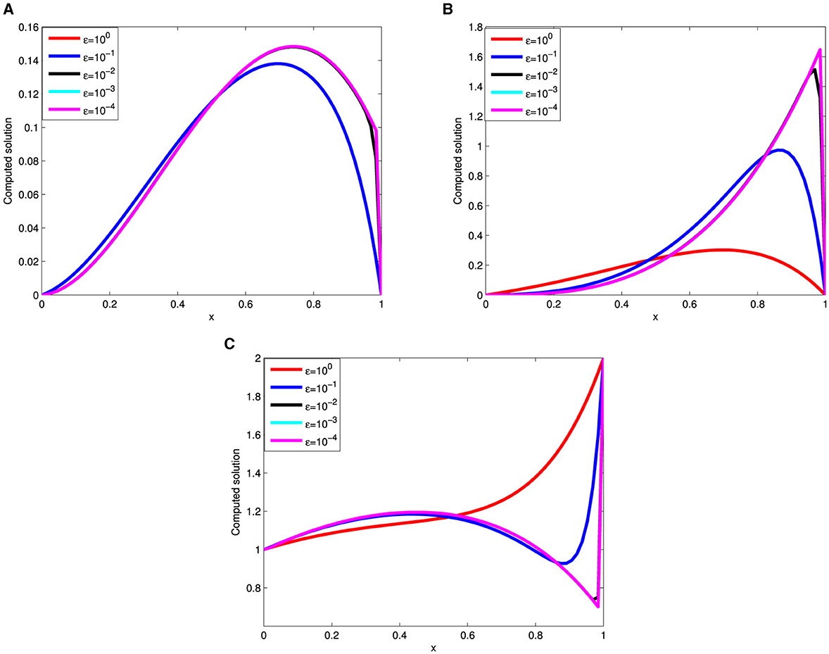
Figure 1. Effect of the ε on solution profile: (A) Example 5.1, (B) Example 5.2, and (C) Example 5.3 for α = 0.5, M = 64, and N = 64, respectively.

Figure 2

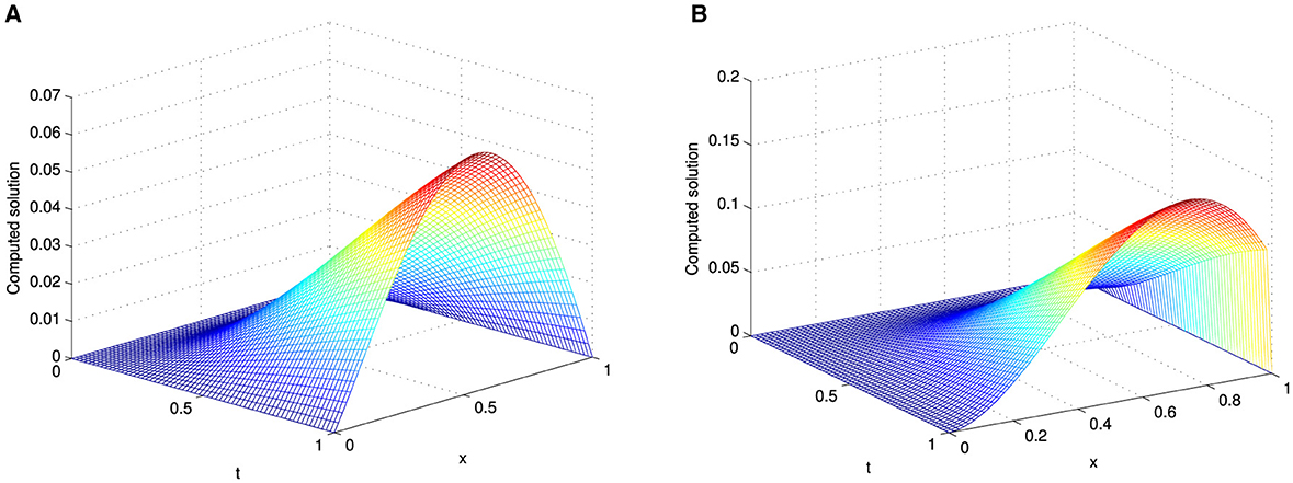
Figure 2. Surface plot of Example 5.1 with M = N = 64, α = 0.5 and (A) for ε = 1 and (B) for ε = 10⁻⁴.

Figure 3

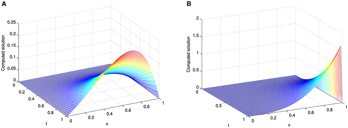
Figure 3. Surface plot of Example 5.2 with M = N = 64, α = 0.5, and (A) for ε = 1 and (B) for ε = 10⁻⁴.

Figure 4

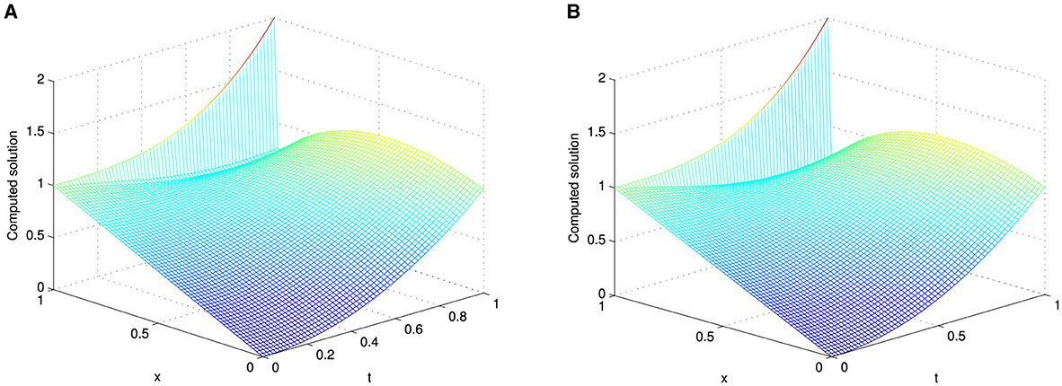
Figure 4. Surface plot of Example 5.3 with M = N = 64, α = 0.5, and (A) for ε = 10⁻² and (B) for ε = 10⁻⁴.

The numerical results in Tables 1–6 illustrate the comparison of the maximum absolute error and order of convergence between the present method and the method presented in Sahoo and Gupta [7] for the considered model examples for different values of α and a fixed ε. In particular, the results in Tables 1, 3, 5 compare the maximum absolute error and order of convergence of the present method with those of the method in Sahoo and Gupta [7] for Examples 5.1–5.3, respectively. The result presented in these tables demonstrate that the present proposed is convergent and more accurate than the method reported in the literature. Tables 7–9 also show the maximum absolute error of the present method for Examples 5.1–5.3, respectively, for a fixed α = 0.5 and varying ε. The numerical results in these tables show that as the perturbation parameter ε approaches to zero, the maximum absolute error of the proposed method stabilizes and becomes consistent after initially increasing. This behavior indicates that the proposed method is parameter uniform, as illustrated in the log-log plots in Figures 5A–C for Tables 7–9, respectively. Finally, the results in Tables 2, 4, 6 present a comparison of the ε-uniform error and ε-uniform rate of convergence for Examples 5.1–5.3, respectively, with the results presented in Sahoo and Gupta [7]. The results presented in these tables clearly demonstrate that the proposed method is more accurate and exhibits a slightly better order of convergence than the method reported in the literature.

Table 1

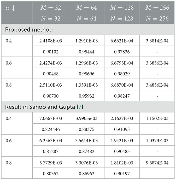
Table 1. $E_{\epsilon }^{M,N}$ and $R_{\epsilon }^{M,N}$ for Example 5.1 with a fixed value of ε = 10⁻⁴ and different values of α.

Table 2

Table 2. E^M,N and R^M,N for Example 5.1 with ε = 10⁻¹⁰ and α = 0.4.

Table 3

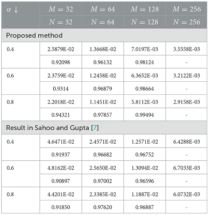
Table 3. $E_{\epsilon }^{M,N}$ and $R_{\epsilon }^{M,N}$ for Example 5.2 for a fixed ε = 10⁻⁴ and different values of α.

Table 4

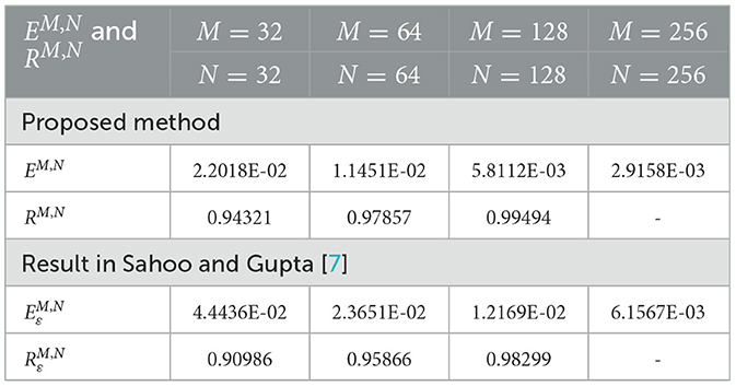
Table 4. E^M,N and R^M,N for Example 5.2 with ε = 10⁻¹⁰ and α = 0.8.

Table 5

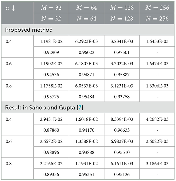
Table 5. $E_{\epsilon }^{M,N}$ and $R_{\epsilon }^{M,N}$ for Example 5.3 for a fixed ε = 10⁻⁴ and different values of α.

Table 6

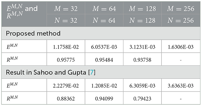
Table 6. E^M,N and R^M,N for Example 5.3 with ε = 10⁻⁴ and α = 0.8.

Table 7

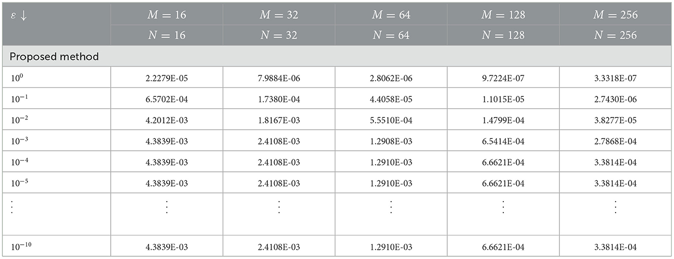
Table 7. $E_{\epsilon }^{M,N}$ for Example 5.1 with a fixed α = 0.4 and different values of ε.

Table 8

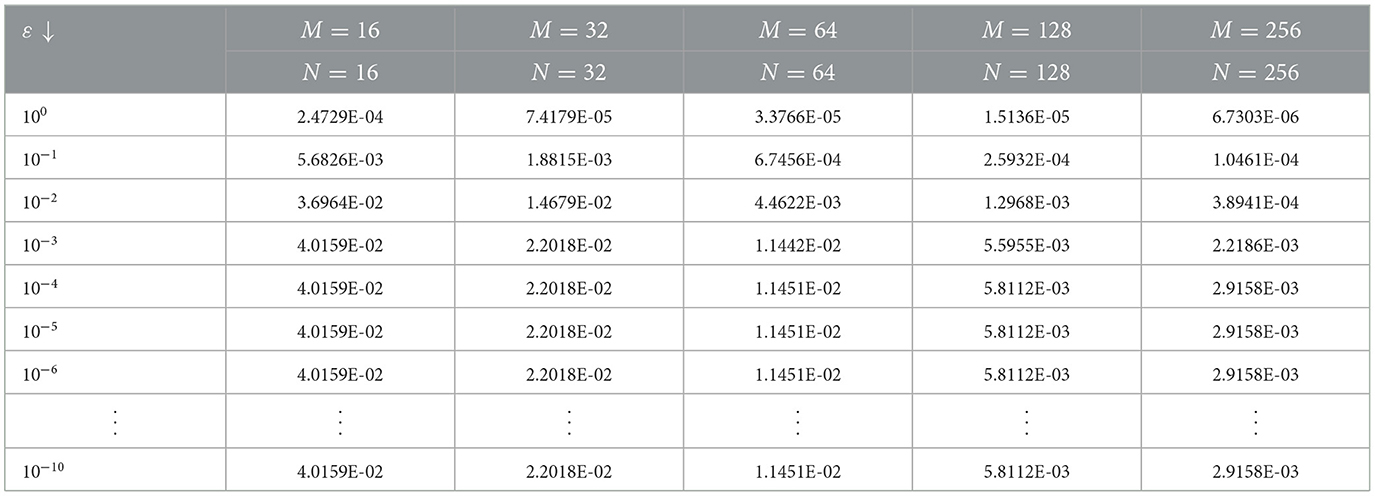
Table 8. $E_{\epsilon }^{M,N}$ for Example 5.2 for a fixed α = 0.8 and different values of ε.

Table 9

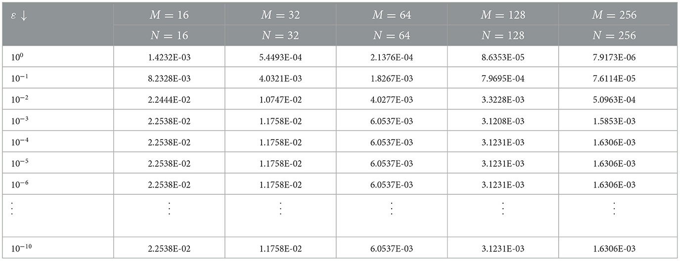
Table 9. $E_{\epsilon }^{M,N}$ for Example 5.3 for a fixed α = 0.8 and different values of ε.

Figure 5

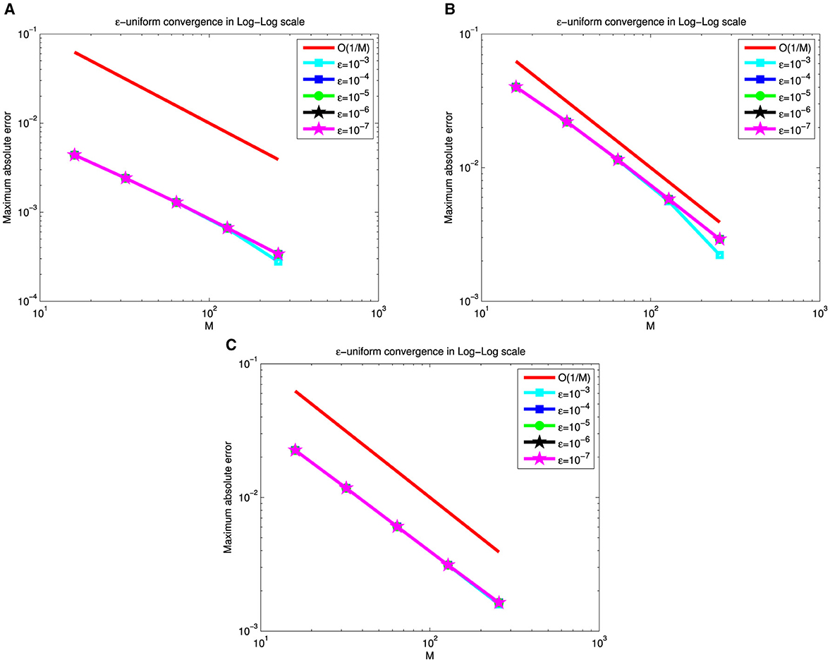
Figure 5. Log-log plot of $E_{\epsilon }^{M,N}$, (A) Example 5.1, (B) Example 5.2, and (C) Example 5.3.

6 Conclusion

A novel exponentially fitted scheme is presented for solving singularly perturbed convection–diffusion problems involving a time-fractional derivative using a Numerov finite-difference approach. The Caputo fraction derivative is used to define the time-fractional derivative and then discretized uniformly using implicit finite difference techniques. Then, an exponentially fitted method is developed using the Numorev finite difference technique along the spatial direction in a uniform mesh discretization. The uniform parameter was rigorously proved, and it is shown to converge with an order of O((Δt)^2−α + M⁻¹). The method is also validated using three model examples, and the experimental results are in agreement with the theoretical expectations. Furthermore, the proposed method provides more accurate solutions than some recently existing results.

Data availability statement

The original contributions presented in the study are included in the article/supplementary material, further inquiries can be directed to the corresponding author.

Author contributions

WA: Conceptualization, Formal analysis, Investigation, Methodology, Software, Resources, Validation, Writing – original draft, Writing – review & editing. GD: Conceptualization, Formal analysis, Investigation, Methodology, Software, Resources, Validation, Supervision Writing – review & editing.

Funding

The author(s) declare that no financial support was received for the research, authorship, and/or publication of this article.

Conflict of interest

The authors declare that the research was conducted in the absence of any commercial or financial relationships that could be construed as a potential conflict of interest.

Generative AI statement

The author(s) declare that no Gen AI was used in the creation of this manuscript.

Publisher's note

All claims expressed in this article are solely those of the authors and do not necessarily represent those of their affiliated organizations, or those of the publisher, the editors and the reviewers. Any product that may be evaluated in this article, or claim that may be made by its manufacturer, is not guaranteed or endorsed by the publisher.

References

1. Anilay WT, Duressa GF, Woldaregay MM. Higher order uniformly convergent numerical scheme for singularly perturbed reaction-diffusion problems. Kyungpook Math J. (2021) 61:591–612. doi: 10.1155/2021/6637661

Crossref Full Text | Google Scholar

2. Woldaregay MM, Aniley WT, Duressa GF. Novel numerical scheme for singularly perturbed time delay convection-diffusion equation. Adv Math Phys. (2021) 2021:6641236. doi: 10.1155/2021/6641236

Crossref Full Text | Google Scholar

3. Tesfaye SK, Woldaregay MM, Dinka TG, Duressa GF. Fitted computational method for solving singularly perturbed small time lag problem. BMC Res Notes. (2022) 15:318. doi: 10.1186/s13104-022-06202-0

PubMed Abstract | Crossref Full Text | Google Scholar

4. Woldaregay M, Aniley W, Duressa G. Fitted numerical scheme for singularly perturbed convection-diffusion reaction problems involving delays. Theor Appl Mech. (2021) 48:171–86. doi: 10.2298/TAM201208006W

Crossref Full Text | Google Scholar

5. Wondimu GM, Duressa GF, Woldaregay MM, Dinka TG. A uniformly convergent computational method for singularly perturbed parabolic partial differential equation with integral boundary condition. J Math Model. (2024) 12:157–75.

Google Scholar

6. Aniley WT, Duressa GF. Uniformly convergent numerical method for time-fractional convection-diffusion equation with variable coefficients. Partial Differ Equ Appl Math. (2023) 8:100592. doi: 10.1016/j.padiff.2023.100592

Crossref Full Text | Google Scholar

7. Sahoo SK, Gupta V. A robust uniformly convergent finite difference scheme for the time-fractional singularly perturbed convection-diffusion problem. Comput Math Appl. (2023) 137:126–46. doi: 10.1016/j.camwa.2023.02.016

Crossref Full Text | Google Scholar

8. Aniley WT, Duressa GF. Nonstandard finite difference method for time-fractional singularly perturbed convection-diffusion problems with a delay in time. Results Appl Math. (2024) 21:100432. doi: 10.1016/j.rinam.2024.100432

Crossref Full Text | Google Scholar

9. Boutiba IM, Baghli-Bendimerad S, El Houda Bouzara-Sahraoui N. Numerical solution by finite element method for time Caputo-fabrizio fractional partial diffusion equation. Adv. Math. Models Appl. (2024) 9:316–328. doi: 10.62476/amma9316

Crossref Full Text | Google Scholar

10. Ma M, Baleanu D, Gasimov YS, Yang XJ. New results for multidimensional diffusion equations in fractal dimensional space. Rom J Phys. (2016) 61:784–94.

Google Scholar

11. Miller KS, Ross B. An Introduction to the Fractional Calculus and Fractional Differential Equations. New York: Wiley (1993).

Google Scholar

12. Oldham K, Spanier J. The Fractional Calculus Theory and Applications of Differentiation and Integration to Arbitrary Order. New York: Academic Press (1974).

Google Scholar

13. Podlubny I. Fractional Differential Equations: An Introduction to Fractional Derivatives, Fractional Differential Equations, to Methods of Their Solution and Some of Their Applications. San Diego: Academic Press (1998).

Google Scholar

14. Kilbas AA, Srivastava HM, Trujillo JJ. Theory and Applications of Fractional Differential Equations, Vol 204. North-Holland: North-Holland Mathematics Studies, Elsevier (2006).

Google Scholar

15. Choudhary R, Singh S, Kumar D. A second-order numerical scheme for the time-fractional partial differential equations with a time delay. Comput Appl Math. (2022) 41:114. doi: 10.1007/s40314-022-01810-9

Crossref Full Text | Google Scholar

16. Choudhary R, Kumar D, Singh S. Second-order convergent scheme for time-fractional partial differential equations with a delay in time. J Math Chem. (2023) 61:21–46. doi: 10.1007/s10910-022-01409-9

Crossref Full Text | Google Scholar

17. Karatay I, Kale N, Bayramoglu S. A new difference scheme for time fractional heat equations based on the Crank-Nicholson method. Fract Calc Appl Anal. (2013) 16:892–910. doi: 10.2478/s13540-013-0055-2

PubMed Abstract | Crossref Full Text | Google Scholar

18. Roul P, Goura VP, Cavoretto R. A numerical technique based on B-spline for a class of time-fractional diffusion equation. Numer Methods Partial Differ Equ. (2023) 39:45–64. doi: 10.1002/num.22790

Crossref Full Text | Google Scholar

19. Yaseen M, Abbas M, Riaz MB. A collocation method based on cubic trigonometric B-splines for the numerical simulation of the time-fractional diffusion equation. Adv Differ Equ. (2021) 2021:1–9. doi: 10.1186/s13662-021-03360-6

Crossref Full Text | Google Scholar

20. Mohyud-Din ST, Akram T, Abbas M, Ismail AI, Ali NH. A fully implicit finite difference scheme based on extended cubic B-splines for time fractional advection–diffusion equation. Adv Differ Equ. (2018) 2018:1–7. doi: 10.1186/s13662-018-1537-7

Crossref Full Text | Google Scholar

21. Rihan FA. Computational methods for delay parabolic and time-fractional partial differential equations. Numer Methods Partial Differ Equ. (2010) 26:1556–71. doi: 10.1002/num.20504

Crossref Full Text | Google Scholar

22. Roul P, Goura VP. A high-order B-spline collocation scheme for solving a non-homogeneous time-fractional diffusion equation. Math Methods Appl Sci. (2021) 44:546–67. doi: 10.1002/mma.6760

Crossref Full Text | Google Scholar

23. Fazio R, Jannelli A, Agreste S. A finite difference method on non-uniform meshes for time-fractional advection-diffusion equations with a source term. Appl Sci. (2018) 8:960. doi: 10.3390/app8060960

PubMed Abstract | Crossref Full Text | Google Scholar

24. Ansari AR, Bakr SA, Shishkin GI. A parameter-robust finite difference method for singularly perturbed delay parabolic partial differential equations. J Comput Appl Math. (2007) 205:552–66. doi: 10.1016/j.cam.2006.05.032

Crossref Full Text | Google Scholar

25. Kumar D, Kumari P. A parameter-uniform numerical scheme for the parabolic singularly perturbed initial boundary value problems with large time delay. J Appl Math Comput. (2019) 59:179–206. doi: 10.1007/s12190-018-1174-z

Crossref Full Text | Google Scholar

26. Bansal K, Sharma KK. Parameter uniform numerical scheme for time dependent singularly perturbed convection-diffusion-reaction problems with general shift arguments. Numer Algor. (2017) 75:113–45. doi: 10.1007/s11075-016-0199-3

Crossref Full Text | Google Scholar

27. Ayele MA, Tiruneh AA, Derese GA. Fitted cubic spline scheme for two-parameter singularly perturbed time-delay parabolic problems. Results Appl Math. (2023) 18:100361. doi: 10.1016/j.rinam.2023.100361

PubMed Abstract | Crossref Full Text | Google Scholar

28. Woldaregay MM, Hunde TW, Mishra VN. Fitted exact difference method for solutions of a singularly perturbed time delay parabolic PDE. Partial Differ Equ Appl Math. (2023) 8:100556. doi: 10.1016/j.padiff.2023.100556

Crossref Full Text | Google Scholar

29. Tesfaye SK, Duressa GF, Dinka TG, Woldaregay MM. Fitted tension spline scheme for a singularly perturbed parabolic problem with time delay. J Appl Math. (2024) 2024:9458277. doi: 10.1155/2024/9458277

Crossref Full Text | Google Scholar

30. Das A, Natesan S. Uniformly convergent hybrid numerical scheme for singularly perturbed delay parabolic convection-diffusion problems on Shishkin mesh. Appl Math Comput. (2015) 271:168–86. doi: 10.1016/j.amc.2015.08.137

Crossref Full Text | Google Scholar

31. Tiruneh AA, Kumie HG, Derese GA. Singularly perturbed time-fractional convection-diffusion equations via exponential fitted operator scheme. Partial Differ Equ Appl Math. (2024) 11:100873. doi: 10.1016/j.padiff.2024.100873

Crossref Full Text | Google Scholar

32. Kumar K, Pramod Chakravarthy P, Vigo-Aguiar J. Numerical solution of time-fractional singularly perturbed convection-diffusion problems with a delay in time. Math Methods Appl Sci. (2021) 44:3080–97. doi: 10.1002/mma.6477

Crossref Full Text | Google Scholar

33. Jain MK, Iyengar SR, Jain RK. Numerical Methods: Problems and Solutions. New Delhi: New Age International (2007).

Google Scholar

34. Adivi Sri Venkata RK, Palli MM. A numerical approach for solving singularly perturbed convection delay problems via exponentially fitted spline method. Calcolo. (2017) 54:943–61. doi: 10.1007/s10092-017-0215-6

Crossref Full Text | Google Scholar