Blessing of dimensionality in spiking neural networks: the by-chance functional learning

Spiking neural networks (SNNs) have significant potential for a power-efficient neuromorphic AI. However, their training is challenging since most of the learning principles known from artificial neural networks are hardly applicable. Recently, the concept of “blessing of dimensionality” has successfully been used to treat high-dimensional data and representations of reality. It exploits the fundamental trade-off between the complexity and simplicity of statistical sets in high-dimensional spaces without relying on global optimization techniques. We show that the frequency encoding of memories in SNNs can leverage this paradigm. It enables detecting and learning arbitrary information items, given that they operate in high dimensions. To illustrate the hypothesis, we develop a minimalist model of information processing in layered brain structures and study the emergence of extreme selectivity to multiple stimuli and associative memories. Our results suggest that global optimization of cost functions may be circumvented at different levels of information processing in SNNs, and replaced by chance learning, greatly simplifying the design of AI devices.

1 Introduction

The exponentially growing demand for computer power in AI already exceeds the progress in developing cutting-edge CMOS technologies [1], which pushes the search for alternative solutions. On the other side, the mammalian brain exhibits unmatched cognitive abilities, consuming only around 20 watts [2]. Thus, a shift of AI to neuromorphic approaches is becoming increasingly imminent [3]. In this context, spiking neural networks (SNNs) may significantly boost the energy efficiency and performance of AI, which is especially relevant for autonomous robotic agents and low-power solutions required, e.g., by the Internet of Things.

One of the most significant issues in developing cognitive, power-efficient SNNs is the problem of their training. It is inextricably linked with choosing one or another specific network architecture and learning paradigm. It turns out that most of the solutions known from artificial neural networks are hardly applicable or simply unfeasible in SNNs [3]. Thus, exploring novel concepts and bioinspired solutions is a significant challenge in the development of SNNs. In this work, we examine two basic frameworks: (1) a simple feedforward architecture equipped with local synaptic plasticity and (2) the blessing of dimensionality in high-dimensional neurons [4]. We show that taking them together can be sufficient for the emergence of by-chance functional selective learning of arbitrary (correlated or not) information items. The by-chance learning relies on a random establishment of links between stimuli and neurons, which are further reinforced through local plasticity (Figure 1). It is effective only when the information items are high-dimensional.

Figure 1

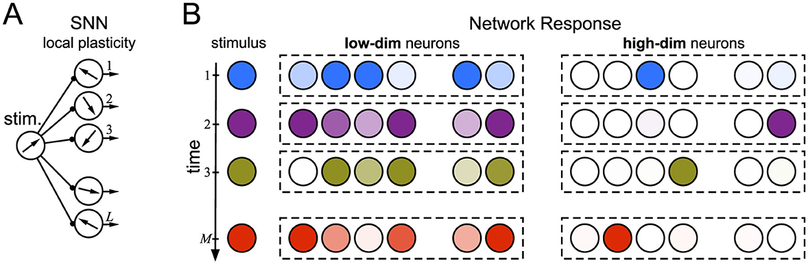
Figure 1. The concept of the by-chance functional learning in a layer of uncoupled spiking neurons operating without global optimization. (A) Shallow network architecture. Stimuli (vectors in a state space) arrive at L ≫ 1 neurons. Each neuron has its own intrinsic characteristic (a vector in “neuronal” space). (B) Sketch of neuron responses to M ≫ 1 sequential stimuli. The neuron response depends on the similarity between the stimulus and neuronal vectors. Stimuli excite random neurons, which in turn learn them locally through Hebbian plasticity. Low-dimensional neurons (left) respond massively and show no specificity to stimuli. High-dimensional neurons (right) become selective, i.e., tied to single stimuli. In the simplest scenario, each neuron responds exclusively to a single stimulus after learning.

The anatomy and connectivity of neural networks influence learning processes. In turn, learning experiences alter neural architecture [5–8]. This dynamic relationship highlights the brain's capacity for neuroplasticity, suggesting that the anatomical framework provides a substrate for learning while the latter induces structural and functional modifications in neural pathways. It creates a continuous feedback loop between structure and experience. Thus, the first steps that will allow model neural networks to approach natural ones should include transitioning from super-deep architectures to shallow ones containing a few layers of high-dimensional neurons (framework 1, Figure 1A). Subsequent steps can involve implementing models of structural plasticity that provide rewiring, consolidating the results of training into long-term memory [8–11].

Following Tyukin et al. [12], we call a neuron high-dimensional if it receives and processes high-dimensional information, i.e., it operates in a multidimensional space (framework 2). Note that a high number of synaptic contacts is a necessary but not sufficient condition. We better refer to the number of “channels” or bundles of axons transmitting statistically independent information. A remarkable brain feature is the ability to learn over a few or even single examples, the so-called one-shot learning [13]. Recent progress in studies of the concentration of measure [14, 15] and stochastic separation theorems [16–19] has laid the theoretical basis for explaining mathematical mechanisms behind this ability. However, the blessing of dimensionality has not been studied in biologically relevant neuronal models. Here, we make a step in closing this gap.

The choice of the learning rule is also important. There is a need to move from global algorithms based on minimizing a loss function to local ones based on the mutual correlation of the activity of interacting neurons. This type of learning, known as Hebbian plasticity [20], implements experimentally discovered effects, such as LTP, LTD, and STDP [for a comprehensive review, see, e.g., [21]]. The application of this approach to the problem of “classical” classification loses to global supervised methods such as gradient descent [3] or to hybrid approaches combining local and global learning [22]. However, Hebbian learning can work in the absence of a large labeled database, implementing the principles of associative learning and self-organizing cognitive neural maps, which has been used, e.g., in neuro-robotics [23–27]. Here, we also stick to biologically justified local learning in the form of synaptic plasticity.

Depending on the specific formulation, Hebbian learning can provide either rate or temporal information coding. Rate coding relies on the spike frequencies, while temporal one focuses on the spike timings. Both strategies have advantages and disadvantages [29]: rate coding is characterized by its simplicity and robustness to noise, making it well-suited for analysis within the framework of local learning in SNNs. Conversely, since temporal coding, implemented, e.g., through the classical STDP rule, can convey information through patterns of timings, it risks being less stable but potentially more reach. Other novel model approaches allow a smooth transition between both types of coding [30, 31]. However, for the sake of simplicity, we restrict ourselves to considering the case of rate-dependent Hebbian plasticity.

2 The problem

2.1 Typical functional organization of an SNN

Figure 2A shows the functional organization of a multilayer neural network typical for the CNS. For example, in the hippocampus, under certain simplifications, single pyramidal neurons in the CA1 layer receive input from different excitatory upstream populations (e.g., ipsi- and contra-lateral CA3, Dentate Gyrus, etc.) and also an inhibitory high-frequency tonic activity from interneurons (e.g., the lacunosum-moleculare layer) [32]. Then, single pyramidal neurons in the target populations (only one is shown in Figure 2A) receive excitatory spike trains from several upstream populations, which conduct information. Besides, the target neurons also receive an inhibitory high-frequency input from local interneurons. The target pyramidal neurons process the external and local information and generate an output. Experimental findings suggest that ongoing learning leads to the formation of spatial modules of coherent activity in the target population [33–35]. In this work, we aim to study learning and the formation of memories in the target population and also understand the role of inhibitory input in this process.

Figure 2

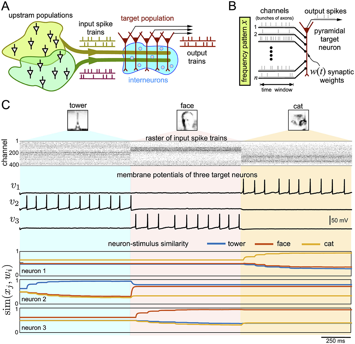
Figure 2. (A) Typical organization of neural networks in the CNS. Upstream populations send spikes through n channels organized in bits of information. (B) Rate coding of information received by a pyramidal neuron in the target population. Vector x defines the frequency pattern, i.e., the frequencies of spikes sent through n channels (bundles of axons). The synaptic weights w define the neuron's responsiveness to the incoming stimuli. It can change over time due to Hebbian plasticity. (C) Response of three pyramidal neurons to three different patterns codifying 20 × 20 px gray-scale images of a tower, a face, and a cat. The raster plot shows spikes in 400 channels (each dot is a spike). The pixel's intensity defines the spiking frequency in the corresponding channel. Traces of the membrane potentials illustrate the spiking activity of the neurons, and colored curves show similarities (Equation 9) of the neurons to three patterns x_{1, 2, 3}.

2.2 Rate coding of information

The upstream populations (Figure 2A) transmit information to target neurons over n channels, which anatomically correspond to bunches of projecting axons. Information is coded in a sequence of discrete time windows of length Δ: [(k − 1)Δ, kΔ), k = 1, 2, … (Figure 2B). According to the frequency or spiking rate coding concept [28, 29, 36], the number of spikes N_jk represents the information contained in the j-th channel and k-th time window. We model the spiking activity in each channel as an independent Poisson point process.

It is convenient to introduce the spiking frequency f_jk = N_jk/Δ and define the information vector:

$\begin{array}{ll}{x}_k={\left(\frac{f_{1k}}{f_{max}},\frac{f_{2k}}{f_{max}},\dots ,\frac{f_{nk}}{f_{max}}\right)}^T\in {\left[0,1\right]}^n,& (1)\end{array}$

where f_max is the maximal frequency of spikes in a channel (i.e., the joint frequency of spikes over all axons in the channel). Following Tyukin et al. [12], we call the target cells, receiving information through n channels, n-dimensional neurons. If n ≫ 1, then neurons are high-dimensional.

We introduce the set of all unique stimuli (information items) for the given target subpopulation (a brain layer may contain many subpopulations):

$\begin{array}{ll}\text{Ω}={\left\{x_i\right\}}_{i=1}^M,& (2)\end{array}$

where M ≫ 1 is the number of stimuli, which can be large but finite (from above, it is restricted by $M\le f_{max}^n$ but in real applications could be much lower).

2.3 Functional learning of information items

As mentioned in the Introduction, learning is a wide concept. We thus restrict the problem to a narrow case. Functional learning occurs if a population of L ≫ 1 pyramidal cells can learn M ≫ 1 arbitrary items of information. We say that an item $x_i\in {\left[0,1\right]}^n$ has been learned if there is a group of neurons exclusively firing to the stimulus x_j and not to all others x_i ∈ Ω\{x_j} (Figure 1B, right).

Let sim(x_i, w) be the similarity operator between the input and some intrinsic features of a neuron (in Section 4.1 we define it for a particular case). Then functional learning assumes:

$\begin{array}{ll}\text{sim}(x_i,w)~1,\text{\hspace{1em}sim}(x_j,w)~0,\forall j\ne i.& (3)\end{array}$

Moreover, sim(x_i + x_j, w) ~ sim(x_i, w) ~ 1, which is the basis for associative learning. If a neuron receives a learned stimulus together with an unknown one, its intrinsic feature w can change to $\tilde{w}$ in such a way that

$\begin{array}{ll}\text{sim}(x_i,\tilde{w})~\text{sim}(x_j,\tilde{w})~1.& (4)\end{array}$

For functional population learning, we require:

1. Adequate response to a novel stimulus (i.e. ∀x ∈ Ω ∃j ∈ {1, …, M} s.t. sim(x, w_j) ~ 1).

2. Reliable learning of a stimulus [i.e., $\text{sim}(x,{\tilde{w}}_j)~1$, where ${\tilde{w}}_j=F(w_j,x)$ and F(·, ·) is a learning operator].

3. Selective learning of a stimulus (i.e., $\text{sim}(y,{\tilde{w}}_j)~0$ ∀y ∈ Ω\{x}).

Below, we develop a mathematical model of the population dynamics and the learning process satisfying these conditions.

3 The model

To study the above-formulated problem (Section 2.3), we introduce a mathematical model describing the dynamics of the target pyramidal neurons and the learning mechanism.

3.1 Dynamics of target pyramidal neurons

To simulate pyramidal neurons, we use the Izhikevich model [37]:

$\begin{array}{l}\frac{dv}{dt}=0.04v^2+5v+140-u-I_{\text{inh}}(t)+I_{\text{exc}}(t)\\ \frac{du}{dt}=a(bv-u)\\ \text{if }v(t)\ge 30\text{then }v(t)\leftarrowtail c,u(t)\leftarrowtail u(t)+d,& (5)\end{array}$

where v is the membrane potential (measured in mV and t is given in ms), u is an auxiliary variable, I_inh(t) and I_exc(t) are the inhibitory and excitatory synaptic currents, respectively. The parameters are set to a = 0.02, b = 0.2, c = −65, and d = 8, corresponding to the “regular spiking” mode.

A tonic high-frequency activity of local interneurons (Figure 2A) produces strongly overlapping inhibitory postsynaptic potentials (IPSPs). Due to the dynamic smoothing, IPSPs, on average, contribute to approximately constant current. Thus, we can set I_inh(t) = γ.

The excitatory current I_exc(t) describes the spiking activity of projecting neurons from the upstream populations (Figure 2A). Assume that information, encoded as spike trains, comes over n channels or bunches of axons (Figure 2B). We use a phenomenological model of a chemical synapse [25, 38]. Let y_j be the synaptic trace for channel j. Then

$\begin{array}{ll}\frac{d{y}_j}{dt}=-\frac{1}{{\tau }_{\text{s}}}{y}_j+{\displaystyle \sum _i}\delta (t-t_{ji}),j=1,\dots ,n,& (6)\end{array}$

where τ_s = 10 ms is the synaptic relaxation time, {t_ji} are the time instants of spikes arriving from this channel, and δ(·) is the delta function. Denoting by $y={(y_1,\dots ,y_n)}^{⊺}$ and by $w={(w_1,\dots ,w_n)}^{⊺}\in {\left[0,1\right]}^n$ the vector of coupling weights for all synaptic channels, we have:

$\begin{array}{ll}{I}_{\text{exc}}(t)=\frac{\beta }{n}\langle w(t),y(t)\rangle ,& (7)\end{array}$

where β is the scaling constant and 〈·, ·〉 stands for the standard inner product.

3.2 Synaptic plasticity in target neurons

The dynamics of the synaptic weights follow the Hebbian type of synaptic plasticity:

$\begin{array}{ll}\frac{dw}{dt}=\mu y_{\text{ps}}(\eta y\circ (1-w)-w),& (8)\end{array}$

where μ is the time-scaling constant, the symbol ° stands for the Hadamard (element-wise) product, y_ps(t) ∈ ℝ is the synaptic trace describing the activity of the pyramidal (postsynaptic) neuron. It obeys the same equation as Equation 6 but with the output spike train $\left\{t_i^{\text{ps}}\right\}$.

Equation 8 is a simplified version of the classical Oja rule [39] and the learning rule used for describing the so-called Concept cells [4]. The first term in the brackets represents learning, while the second implements forgetting. Thus, η is the relative learning-forgetting rate. We note that both learning and forgetting occur only when the pyramidal neuron is active, i.e., y_ps>0.

4 Decoding and learning information items

4.1 Simple example of functional learning

Figure 2C shows the response of three pyramidal neurons in the target population to a sequence of three stimuli codifying 20 × 20 pixel images of a tower, a face, and a cat. The pixel's brightness corresponds to the frequency of spikes sent by the upstream populations through a channel (raster plot of spikes in Figure 2C). Each stimulus lasts for 1 s, and each neuron either fires spikes to a stimulus or not. Firing a spike means that a neuron detects (recognizes) a stimulus.

Initially, the pyramidal neurons have arbitrary synaptic weights w_i (i = 1, 2, …, L; in Figure 2C, L = 3). Since the synaptic current (7) depends on the inner product, it is convenient to define the similarity operator used in Section 2.3 between the neuron's weights w_i(t) and the stimulus pattern x_j as:

$\begin{array}{ll}\text{sim}(x_j,w_i(t)):=\frac{\langle x_j,w_i(t)\rangle }{||x_j||||w_i(t)||}\in \left[0,1\right].& (9)\end{array}$

If sim(x_j, w_i(t)) = 1 then the stimulus and the neuron are collinear, whereas for sim(x_j, w_i(t)) = 0 they are orthogonal.

Consider the dynamics of the membrane potential of neuron 1, v₁(t) (Figure 2C). We observe that the neuron stays inactive for the first two patterns (the tower and face), but it detects the cat's image by generating spikes. Such a behavior can be explained by checking the similarities between w₁(t) and the patterns x_{1, 2, 3} (Figure 2C, neuron-stimulus similarity). The similarities sim(x₁, w₁) and sim(x₂, w₁) are low, while sim(x₃, w₁) is higher. Therefore, the neuron “skips” the first two stimuli but detects the third one. Note that once the neuron generates postsynaptic spikes, its synaptic trace becomes positive, y_ps>0, and learning occurs (Equation 8). The synaptic weights are tuned so that the similarity to the cat's image becomes even higher (in a series of exponential steps) while the similarity to the tower and the face becomes lower. Thus, after learning, the neuron becomes even more prone to firing in response to the cat's image and ignoring the tower and face. Similar situations occur with neurons 2 and 3 (Figure 2C). They also tune in to their stimuli. Thus, we have a basic example of functional learning.

4.2 Replication of frequency patterns at single synapses

Let us study functional learning in detail. In a single time window, if a pattern x does not excite a neuron, then no learning occurs, and the synaptic weights stay unchanged. In this case, the neuron “waits” for another pattern that will activate it. For example, in Figure 2C, neuron 1 skips two patterns and only then fires to the third information item, the cat.

Assume that a neuron fires to pattern x ∈ Ω, i.e., y_ps(t) > 0 for t > t^*, and hence learning occurs. Then, the synaptic trace y(t) is determined by n Poisson point processes with the expected value (Appendix 1):

$\begin{array}{ll}\text{E}\left[y\right](t)=f_{max}{\tau }_s\left(1-e^{-\frac{t}{{\tau }_s}}\right)x.& (10)\end{array}$

Thus, on average, the synaptic signal y is proportional to the input pattern x.

Approximating the synaptic trace y by its expectation (Equation 10), for t ≫ τ_s (in simulations τ_s = 10 ms, Δ = 10³ ms), we can find the mean synaptic weights after learning for a single target neuron (Appendix 1):

$\begin{array}{ll}{w}^{*}=x\oslash (\alpha +x),\alpha =\frac{1}{\eta {\tau }_s{f}_{max}},& (11)\end{array}$

where ⊘ stands for the Hadamard division. Thus, the synaptic weights are uniquely defined by the stimulus pattern, i.e., by the frequencies of incoming spike trains, and depend on the learning-forgetting rate η.

To test the theoretical prediction, we simulated the neuronal response to a pattern codified by n = 100 spike trains with frequencies ranging from 1 to 10³ Hz. The synaptic weights at the beginning were distributed randomly (w(0) ~ U¹⁰⁰[0, 1]). The learning protocol lasted 1 s of the model time.

Figure 3 shows the synaptic weights after learning vs. the spike frequency in the corresponding synaptic channel. As expected, after a transient process, the synaptic weights stabilize at the values provided by Equation 11. Thus, learning leads to replicating the frequency rates at the synapses. This replication is one-to-one but nonlinear.

Figure 3

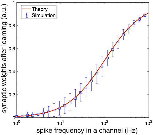
Figure 3. Learning causes synaptic replication of frequency patterns. A pyramidal neuron with random synaptic weights is activated by a pattern with spike frequencies in the range [1, 10³] Hz. After learning, synaptic weights replicate the frequencies of spike trains in the pattern following Equation 11. Parameter values: η = 1, μ = 0.05, γ = 10, β = 17, τ_s = 10 ms, $f_{max}=10^3$ Hz, n = 100.

4.3 Functional population learning

The model neuron (5), like most biological ones, has no hard threshold [37]. At I(t) = I_exc(t) − I_inh(t) ≈ 2.6, it generates a single spike, and for I(t) ≈ 3.8, the model starts generating a spike train. We define θ ≈ 2.6 as the “soft” firing threshold for convenience, although its exact value depends on the model dynamics.

Let us now consider the target population of L pyramidal neurons (Figure 2A, L ≫ 1). At t = 0, the population stores no a priori information, i.e., the synaptic weights of all neurons are taken i.i.d. from a uniform distribution:

$\begin{array}{ll}{w}_i(t=0)~U^n\left[0,1\right],i=1,2,\dots ,L.& (12)\end{array}$

Then, all neurons receive the same stimuli as a sequence of frequency patterns, and the target population must exhibit functional learning (Section 2.3).

4.3.1 Adequate response to a novel stimulus

If L ≫ 1, given a pattern x, some target neurons may fire by chance (e.g., in Figure 2C, one neuron fires to one pattern). A neuron fires to the pattern if it consistently has I(t)>θ in the corresponding time interval. The total synaptic current depends on the pattern-synaptic match [directly related to the similarity (9)]:

$\begin{array}{ll}{\rho }_i:=\frac{\langle x,w_i\rangle }{n}\in \left[0,1\right].& (13)\end{array}$

If the match is high, the likelihood of firing in response to x is higher. In general, stimulus vectors, i.e., the set Ω, can follow an arbitrary distribution. Then, we use the most natural assumption x~Uⁿ[0, 1]. Note that concentration properties apply to such stimuli, however, other distributions, e.g., defined on a ball, can also be used [17]. Using Definition (Equation 13), we get the probability of firing (Appendix 2.1):

$\begin{array}{ll}{P}_{\text{new}}=\text{Φ}\left(\sqrt{9n/7}(1-\text{λ})\right),& (14)\end{array}$

where Φ(·) is the normal cumulative distribution function and

$\begin{array}{ll}\text{λ}:=4\frac{\theta +\gamma }{\beta {\tau }_s{f}_{max}},& (15)\end{array}$

is the inhibitory-excitatory ratio of the synaptic currents. The probability (Equation 14), defines the mean ratio of excited neurons in the target population firing to a novel stimulus.

Figure 4A (black curve) illustrates the firing probability to a novel stimulus as a function of the inhibitory-excitatory ratio evaluated numerically and using Equation 14. We observe a tide correspondence between theory and simulations. As expected, increasing the inhibition γ (and hence λ) decreases the probability of the first firing to a novel stimulus in the target population. For example, for λ = 1, about 50% of the pyramidal neurons respond to a novel stimulus, while for λ = 1.2 the ratio falls to 1.2%. As discussed below, Equation 14 allows suitable selection of parameters for functional learning.

Figure 4

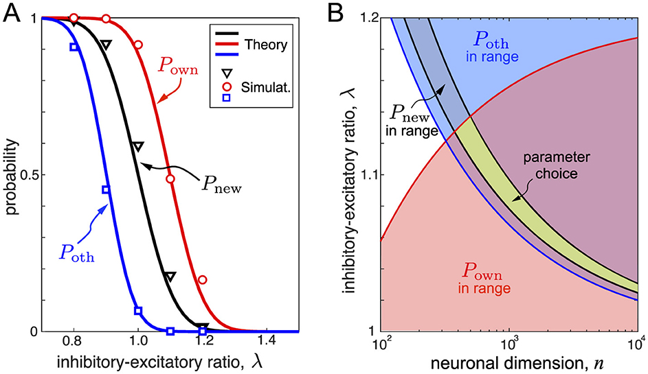
Figure 4. Optimal learning requires matching main neuronal features. (A) Probabilities of firing of target neurons to stimuli vs the inhibitory-excitatory ratio. Black, red, and blue colors correspond to novel stimuli, own stimuli after learning, and other stimuli, respectively (symbol markers show the results of numerical simulations, curves correspond to Equations 14, 17, 19). Parameter values: n = 100, η = 0.2, and μ = 0.4. (B) Areas of the neuronal parameters suitable for functional learning delimited by inequalities (Equations 23–25). The green area corresponds to optimal functional learning. Note that P_new, as the probability of firing to a novel stimulus, imposes conditions on the SNN before learning, while P_own and P_oth define the SNN response after learning. Parameter value: η = 0.25.

4.3.2 Reliable learning of an arbitrary pattern

If a neuron generates spikes in response to stimulus x, learning occurs, and its synaptic weights converge to the values given by Equation 11. In general, the neuron becomes even more tied to the stimulus after learning, i.e., if the same stimulus appears again, the neuron will fire more strongly. However, such an intuition can fail, and the neuron can stop firing in response to x. It happens if the pattern-synaptic match (Equation 13) after learning is too small and, hence, the total synaptic current falls below the threshold I(t) < θ.

After learning, the pattern-synaptic match is:

$\begin{array}{ll}{\rho }_{\text{lrn}}(x,\alpha )=\frac{\langle x,x\oslash (\alpha +x)\rangle }{n}.& (16)\end{array}$

It is a decreasing function of α. Thus, α must be small enough, which can be achieved by raising the learning-forgetting ratio η (Equation 11).

The conditional probability of firing to the learned stimulus is (Appendix 2.2):

$\begin{array}{ll}{P}_{\text{own}}:=P(\text{fire to }x|\text{learned }x)=\text{Φ}\left((f_1(\alpha )-\text{λ}/4)\sqrt{n/f_2(\alpha )}\right),& (17)\end{array}$

where

$\begin{array}{r}{f}_1(\alpha )=\frac{1}{2}-\alpha +{\alpha }^{2}ln(1+{\alpha }^{-1}),\\ f_2(\alpha )=\frac{4}{3}-f_1(\alpha )(f_1(\alpha )+4\alpha )-\frac{1}{\alpha +1},& (18)\end{array}$

are positive decreasing functions of α. Figure 4A (in red) shows the probability of firing to the learned stimulus. Reliable learning requires high P_own and hence a moderate inhibitory-excitatory ratio.

4.3.3 Selective response to stimuli

Learning a pattern also changes the probability of firing to other stimuli. For selective learning, we require that, after learning item x, the neuron fires spikes to this item but at the same time will be silent to other items from Ω\{x}.

The probability to fire to stimulus ξ after learning x (ξ≠x) is (Appendix 2.3):

$\begin{array}{ll}{P}_{\text{oth}}:=P(\text{fire to }\xi |\text{learned }x)=\text{Φ}\left((f_3(\alpha )-\text{λ}/4)\sqrt{n/f_4(\alpha )}\right),& (19)\end{array}$

where

$\begin{array}{ll}\begin{array}{c}{f}_3(\alpha )=\frac{1}{2}(1-\alpha log(1+{\alpha }^{-1})),\\ f_4(\alpha )=\frac{4}{3}{f}_3(\alpha )-f_3^2(\alpha )-\frac{1}{3(\alpha +1)},\end{array}& (20)\end{array}$

are positive decreasing functions of α. Figure 4A (blue curve) illustrates how the probability (Equation 19) changes with λ. This probability must be low enough for optimal learning, which can be achieved by increasing the inhibitory-excitatory ratio.

4.3.4 Conditions for optimal learning

For meaningful functional learning (Section 2.3), the probabilities P_new, P_own, and P_oth must be appropriately selected. For example, for λ = 1, P_new = 1/2, and half of the neurons in the target population learn the first incoming stimulus. Then, the second stimulus will take 25% of the remaining neurons, the third 12.5%, etc. Thus, in a few steps, we run out of neurons. Such a situation is far from optimal, and hence, we must increase the inhibitory-excitatory ratio λ.

For λ = 1.2, the probability of firing to a novel stimulus is 0.01, which may be acceptable. However, for the same λ, P_own≈0.1 (Figure 4A), and neurons, after learning, will not fire to the learned stimuli. Thus, the situation shown in Figure 4A is not optimal for functional population learning. Therefore, the parameter choice must be compatible with conditions imposed on all three probabilities P_new, P_own, and P_oth.

To remedy the problem, first, the neuronal population must have the probability of firing to an arbitrary stimulus within some range. This range depends on the population size L and the desired number of stimuli to be learned M. The expected number of neurons firing to the i-stimulus is $L{P}_{\text{new}}{(1-P_{\text{new}})}^{i-1}$. Thus, if the target population must learn up to M items, the population size must satisfy the condition:

$\begin{array}{ll}L>\frac{1}{P_{\text{new}}{(1-P_{\text{new}})}^{M-1}},& (21)\end{array}$

which sets the condition for P_new:

$\begin{array}{ll}{P}_{\text{new}}\in (p_0,p_1).& (22)\end{array}$

For example, considering learning of 1,000 items by a population of 5,000 neurons, we get $p_0=2.6\times 10^{-4}$ and $p_1=2.5\times 10^{-3}$.

Equation 22 sets a condition on the inhibitory-excitatory balance λ and the neuronal dimension n:

$\begin{array}{ll}1-\frac{\sqrt{7}{\text{Φ}}^{-1}(p_1)}{3\sqrt{n}}<\text{λ}<1-\frac{\sqrt{7}{\text{Φ}}^{-1}(p_0)}{3\sqrt{n}}.& (23)\end{array}$

Note that the available range decreases as $1/\sqrt{n}$.

Besides, we require that a target neuron, after learning, must fire to the learned stimulus with a high enough probability P_own > p₂. Then, from Equation 17, we get the condition:

$\begin{array}{ll}\text{λ}<4f_1(\alpha )-\frac{4{\text{Φ}}^{-1}(p_2)\sqrt{f_2(\alpha )}}{\sqrt{n}}.& (24)\end{array}$

Moreover, the neuron must be selective, i.e., the probability of firing to other stimuli must be low enough, P_oth < p₃:

$\begin{array}{ll}\text{λ}>4f_3(\alpha )-\frac{4{\text{Φ}}^{-1}(p_3)\sqrt{f_4(\alpha )}}{\sqrt{n}}.& (25)\end{array}$

where the upper bound can be set to p₃ = 1/M.

Figure 4B shows the regions satisfying conditions (Equations 23–25). The intersection of the three regions provides the optimal choice of the parameters (green area in Figure 4B). We observe that there is a minimal neuronal dimension n below which neurons cannot be selective. This result is in qualitative accordance with the main conclusion of the analysis of formal neurons [4, 12]. However, n must not be too high for relatively small populations. Otherwise, the inhibitory-excitatory balance must be selected extremely precisely, which is not biologically plausible. The latter feature is particular to spiking neurons.

4.4 Selective decoding of information by pyramidal neurons

Let us now illustrate how the population of pyramidal neurons with parameters satisfying the selective criteria (Figure 4B) can learn to decode the incoming information efficiently. We use the CIFAR-10 database consisting of 32 × 32 pixel natural images [40] as a source of the information items. We take photos of cats from the database (i.e., a single class of images; note that here we are not interested in the classification problem, but in a highly selective response of a layer of target neurons). Besides, the original images are in color, and we converted them into grayscale pictures.

Natural images usually have peaked distributions of pixels depending on the lighting conditions at the time of the shot. Figure 5A (left) shows examples of two photos and the corresponding distributions. The distributions significantly deviate from uniform, which is used as the standard, while we have developed the theoretical predictions. Thus, we applied a simple preprocessing step to homogenize the pixel distributions. Figure 5A (right) shows the resulting images and their flat distributions. Note that the normalized images gain contrast and visually exhibit more details than the original ones. Such a transformation, optimizing the image contrast, occurs at different levels in the visual system, from pupil dilation to changes in cortical processing [for details see, e.g., [41]]. It also applies to computer vision and modern event-based cameras [3, 42].

Figure 5

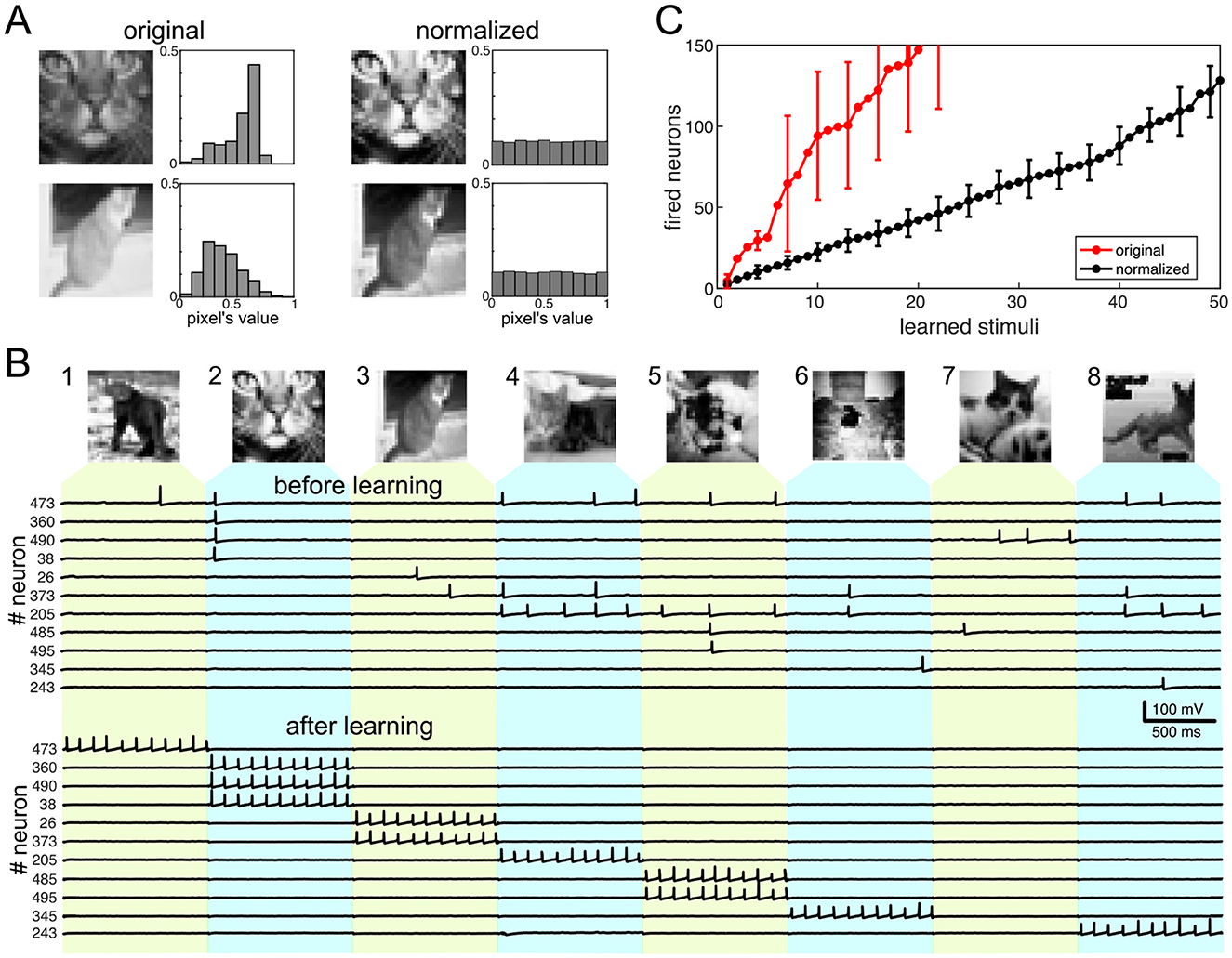
Figure 5. Emergence of functional learning in a population of pyramidal cells. (A) Example of normalization of two pictures of cats (32 × 32 gray-scale images from the CIFAR-10 database). After normalization, the pixels' distribution is flat. (B) Learning the first eight images of cats. Top: Images of cats used for learning. Middle: Spike trains of 11 neurons firing to the eight stimuli before learning. Bottom: Spike trains of the same neurons but after learning. The neurons fired to the eight images are ordered according to the image number. (C) The use of neurons for learning stimuli. The black curve corresponds to normalized images, while the red one shows the number of neurons firing to original images. Vertical bars show standard deviation. Parameter values: $f_{max}=10^3$ Hz, τ_s = 10 ms, γ = 10, η = 0.22, μ = 1.2.

To get stimulus vectors, we flatten the images (by aligning all columns of a matrix representing the image into a single column vector), thus getting $x_i\in {\left[0,1\right]}^{1,024}$. Such a high neuronal dimension is expected to guarantee the blessing of the dimensionality phenomenon (predicted in Section 4.3.4). We consider a target population of M = 500 pyramidal neurons in simulations. At t = 0, the neurons have random synaptic weights (i.e., $w_i~U{\left[0,1\right]}^n$, i = 1, …, M) and, hence, no specific relations to the stimuli. Then, stimulus vectors have been applied to the pyramidal neurons in a sequence, and the nonlinear dynamics of the target population has been simulated (Section 3).

Figure 5B illustrates the population response to the first eight images. We run the algorithm twice. First, learning has been switched off by setting μ = 0. It has been used to test how the population responds to stimuli without learning. As expected, the neuronal firing is random along the selected neurons and images. The eleven traces of the membrane potentials shown in Figure 5B (before learning) correspond only to those neurons that fire spikes in response to the eight stimuli.

Although before learning, neurons fire arbitrarily and have no preferences for the stimuli, such a disordered firing plays an important role. It promotes learning of the patterns by chance. Neurons with synaptic weights close to a given stimulus will fire on its presentation. The expected number of such neurons is given by P_newM, which is relatively small, and hence, the firing frequency is low in the target population before learning.

Although before learning, neurons fire arbitrarily and have no preferences for the stimuli, such a disordered firing plays an important role. It promotes learning of the stimuli by chance. Neurons with synaptic weights close to a given stimulus (in terms of Equation 13) will fire on its presentation. The expected number of such neurons is P_newM, which is relatively small, and hence, the firing frequency in the target population before learning is low.

To study the learning process, the second run of the model has been performed with μ = 1.2. Then again, we checked the firing activity in the population (Figure 5B, after learning). Neurons that fire to a stimulus learn the stimulus, but only a fraction of them, given by P_own, will keep firing after learning (Section 4.3). Thus, after learning, we can have about P_ownP_initM neurons firing to the given stimulus. Since P_own is selected to be high, most neurons will be tied to the stimuli that excited them initially. After learning, neurons fire tonic spikes to their stimuli (Figure 5B, after learning). Besides, we can observe a situation that happens with the seventh image. Although neurons 490 and 485 fire spikes to this stimulus before learning, these neurons learn stimuli 2 and 5, which come before the seventh. Thus, they significantly change their synaptic weights, and the pattern-synaptic matching becomes low for stimulus 7. Finally, no neuron learns the 7th image. Therefore, the target population can miss some stimuli.

The next observation is the selectivity of neurons to the learned stimuli. A neuron that learned a stimulus is selective, i.e., it ignores all the other M−1 stimuli, with the probability:

$\begin{array}{ll}{P}_{\text{slc}}={(1-P_{\text{oth}})}^{M-1}.& (26)\end{array}$

This probability can be close to 1 if P_oth is small enough, which is ensured by the conditions for optimal learning (Section 4.3.4). Then, after learning, neurons in the population will fire to single stimuli and be silent to all other images.

Finally, we tested the number of neurons necessary for learning a sequence of stimuli (Figure 5C). First, we used images with a uniform distribution (Figure 5A, right). The number of neurons fired in response to stimuli (Figure 5C, black curve) increased almost linearly with a slope of 2.41 neurons per new stimulus. We then conducted the same calculations with the original images. In this case, to maintain the excitatory postsynaptic potential (EPSP) in the target neurons, we adjusted the maximal frequency of spikes based on the mean image intensity. The resulting curve (Figure 5C, in red) showed a significantly steeper slope and exhibited strong oscillations. This finding suggests that the initial relay stations of the visual system must preprocess raw images before the corresponding stimuli enter brain layers performing functional learning. This aligns with experimental findings. Additionally, we observed that the number of neurons in a processing chunk must be considerably higher than the number of stimuli for effective learning, which directly relates to the neuronal dimension.

5 Conclusions

The human brain exhibits an unprecedented ability for power-efficient cognitive learning that is unreachable for modern AI. This pushes research in neuromorphic neural networks that can become a substrate for the next generation of AI. In this work, we introduced a spiking neural network model and studied functional learning. The goal was to leverage the simple layered “anatomy” and local plasticity of the SNN and the phenomenon of blessing of dimensionality.

Despite the model's simplicity, we have shown that it enables functional learning, given that several crucial features are fulfilled. The SNN can selectively learn arbitrary information (images of cats from the CIFAR-10 database have been used in numerical simulations as examples of information items). This is a crucial step for associative learning of unrelated items and, more importantly, breaking associations between related items when needed.

We have shown that the feedforward anatomy can be sufficient for local learning. Thus, no bulky, biologically questionable mechanisms of global optimization (e.g., back-propagation with gradient descent) are required. Instead, target neurons can learn stimulus items “by chance.” In other words, neurons in a chunk belonging to the target layer have random synaptic weights at the beginning and fire randomly to the incoming stimuli. If the number of neurons is high enough and the probability of firing is balanced, we get a few neurons firing to a stimulus. These neurons learn the stimulus, and the procedure is repeated for the next novel stimulus.

We have shown that by-chance learning works if the inhibitory-excitatory balance and the learning-forgetting ratio are within adequate limits. Thus, local tonic inhibition observed in different layered brain structures, including the neocortex, is necessary for learning. The blessing of dimensionality also plays a crucial role. It is necessary for selective learning, i.e., when a brain structure, e.g., the medial temporal lobe, must selectively “recognize” different information items. This is the case of the so-called Jennifer Aniston neuron [43].

However, we also observed a crucial difference with the earlier results on artificial neural networks. It turns out that the neuronal dimension must not be too high. Otherwise, the inhibitory-excitatory balance and the learning-forgetting rate must be tuned with high precision. This observation has indirect experimental support. The CA1 layer in the hippocampus is anatomically homogeneous but has a functionally modular structure [35], probably dedicated to processing disjoint blocks of information. The modular size varies significantly for different neuronal pathways. Using theoretical [44] and experimental [35] studies, an estimate gives 2,000 and 15,000 pyramidal neurons per module for the MPP entorhinal and Schaffer generators, respectively. It agrees with our predictions on the optimal number of neurons. Moreover, the upper bound on the input dimension may explain why neurons receiving extremely high-dimensional input, such as Purkinje cells playing a critical role in motor coordination, cannot be selective.

We also found some limitations of the model due to its simplicity. For example, learning large stimulus sequences requires an exponentially increasing number of neurons. This can be mediated either by using chunks of neurons or lateral inhibition. Both options are known in neuroscience [45]. Besides, learning can be more stable if the local inhibition can be modulated by incoming spike trains. It can be remedied by homeostatic plasticity [46]. These and other questions open new lines for further research.

Data availability statement

The datasets and Appendices presented in this study can be found in online repositories. The names of the repository/repositories and accession number(s) can be found in the article/Supplementary material.

Author contributions

VM: Conceptualization, Data curation, Investigation, Methodology, Software, Supervision, Writing – original draft, Writing – review & editing. SL: Conceptualization, Investigation, Methodology, Writing – original draft, Writing – review & editing.

Funding

The author(s) declare that financial support was received for the research and/or publication of this article. This work has been supported by the Spanish Ministry of Science and Innovation (Project No. PID2021-124047NB-I00) and by the Russian Science Foundation (project 24-19-00433).

Conflict of interest

The authors declare that the research was conducted in the absence of any commercial or financial relationships that could be construed as a potential conflict of interest.

The author(s) declared that they were an editorial board member of Frontiers, at the time of submission. This had no impact on the peer review process and the final decision.

Generative AI statement

The author(s) declare that no Gen AI was used in the creation of this manuscript.

Publisher's note

All claims expressed in this article are solely those of the authors and do not necessarily represent those of their affiliated organizations, or those of the publisher, the editors and the reviewers. Any product that may be evaluated in this article, or claim that may be made by its manufacturer, is not guaranteed or endorsed by the publisher.

Supplementary material

The Supplementary Material for this article can be found online at: https://www.frontiersin.org/articles/10.3389/fams.2025.1553779/full#supplementary-material

References

1. Mehonic A, Ielmini D, Roy K, Mutlu O, Kvatinsky S, Serrano-Gotarredona T, et al. Roadmap to neuromorphic computing with emerging technologies. APL Mater. (2024) 12:109201. doi: 10.1063/5.0179424

Crossref Full Text | Google Scholar

2. Javed F, He Q, Davidson LE, Thornton JC, Albu J, Boxt L, et al. Brain and high metabolic rate organ mass: contributions to resting energy expenditure beyond fat-free mass. Am J Clin Nutr. (2010) 91:907–12. doi: 10.3945/ajcn.2009.28512

PubMed Abstract | Crossref Full Text | Google Scholar

3. Makarov VA, Lobov SA, Shchanikov S, Mikhaylov A, Kazantsev VB. Toward reflective spiking neural networks exploiting memristive devices. Front Comput Neurosci. (2022) 16:859874. doi: 10.3389/fncom.2022.859874

PubMed Abstract | Crossref Full Text | Google Scholar

4. Calvo Tapia C, Tyukin I, Makarov VA. Universal principles justify the existence of concept cells. Sci Rep. (2020) 10:7889. doi: 10.1038/s41598-020-64466-7

PubMed Abstract | Crossref Full Text | Google Scholar

5. Edelman GM. Neural darwinism: selection and reentrant signaling in higher brain function. Neuron. (1993) 10:115–25. doi: 10.1016/0896-6273(93)90304-A

PubMed Abstract | Crossref Full Text | Google Scholar

6. Friston KJ. Functional and effective connectivity: a review. Brain Connect. (2011) 1:13–36. doi: 10.1089/brain.2011.0008

PubMed Abstract | Crossref Full Text | Google Scholar

7. Floreano D, Dürr P, Mattiussi C. Neuroevolution: from architectures to learning. Evol Intell. (2008) 1:47–62. doi: 10.1007/s12065-007-0002-4

Crossref Full Text | Google Scholar

8. Calvo Tapia C, Makarov VA, van Leeuwen C. Basic principles drive self-organization of brain-like connectivity structure. Commun Nonlinear Sci Numer Simul. (2020) 82:105065. doi: 10.1016/j.cnsns.2019.105065

Crossref Full Text | Google Scholar

9. Shen J, Xu Q, Liu JK, Wang Y, Pan G, Tang H, et al. an evolutionary structure learning strategy for spiking neural networks. Proc AAAI Conf Artif Intell. (2023) 37:86–93. doi: 10.1609/aaai.v37i1.25079

PubMed Abstract | Crossref Full Text | Google Scholar

10. Lobov SA, Berdnikova ES, Zharinov AI, Kurganov DP, Kazantsev VB. STDP-driven rewiring in spiking neural networks under stimulus-induced and spontaneous activity. Biomimetics. (2023) 8:320. doi: 10.3390/biomimetics8030320

PubMed Abstract | Crossref Full Text | Google Scholar

11. Lobov SA, Zharinov A, Kurganov D, Kazantsev VB. Network memory consolidation under adaptive rewiring. Eur Phys J Spec Top. (2025). doi: 10.1140/epjs/s11734-025-01595-y

Crossref Full Text | Google Scholar

12. Tyukin I, Gorban AN, Calvo C, Makarova J, Makarov VA. High-dimensional brain: a tool for encoding and rapid learning of memories by single neurons. Bull Math Biol. (2019) 81:4856–88. doi: 10.1007/s11538-018-0415-5

PubMed Abstract | Crossref Full Text | Google Scholar

13. Lake BM, Salakhutdinov R, Tenenbaum JB. Human-level concept learning through probabilistic program induction. Science. (2015) 350:1332–8. doi: 10.1126/science.aab3050

PubMed Abstract | Crossref Full Text | Google Scholar

14. Kainen P, Kurková V. Quasiorthogonal dimension of euclidean spaces. Appl Math Lett. (1993) 6:7–10. doi: 10.1016/0893-9659(93)90023-G

Crossref Full Text | Google Scholar

15. Kainen PC. (1997) “Utilizing geometric anomalies of high dimension: when complexity makes computation easier.” In:Karny M, Warwick K, , editors. Computer Intensive Methods in Control and Signal Processing. Springer: New York. doi: 10.1007/978-1-4612-1996-5_18

Crossref Full Text | Google Scholar

16. Gorban A, Tyukin I. Stochastic separation theorems. Neur Net. (2017) 94:255–9. doi: 10.1016/j.neunet.2017.07.014

PubMed Abstract | Crossref Full Text | Google Scholar

17. Gorban AN, Makarov VA, Tyukin IY. The unreasonable effectiveness of small neural ensembles in high-dimensional brain. Phys Life Rev. (2019) 29:55–88. doi: 10.1016/j.plrev.2018.09.005

PubMed Abstract | Crossref Full Text | Google Scholar

18. Gorban AN, Makarov VA, Tyukin IY. High-dimensional brain in a high-dimensional world: blessing of dimensionality. Entropy. (2020) 22:82. doi: 10.3390/e22010082

PubMed Abstract | Crossref Full Text | Google Scholar

19. Kreinovich V, Kosheleva O. Limit theorems as blessing of dimensionality: neural-oriented overview. Entropy. (2021) 23:501. doi: 10.3390/e23050501

PubMed Abstract | Crossref Full Text | Google Scholar

20. Hebb DO. The Organization of Behavior: A Neuropsychological Theory. New York: Wiley (1949).

Google Scholar

21. Markram H, Gerstner W, Sjöström PJ. A history of spike-timing-dependent plasticity. Front Synaptic Neurosci. (2011) 3:4. doi: 10.3389/fnsyn.2011.00004

PubMed Abstract | Crossref Full Text | Google Scholar

22. Shen J, Ni W, Xu Q, Pan G, Tang H. Context gating in spiking neural networks: achieving lifelong learning through integration of local and global plasticity. Knowl-Based Syst. (2025) 311:112999. doi: 10.1016/j.knosys.2025.112999

Crossref Full Text | Google Scholar

23. Krichmar JL, Edelman GM. Machine psychology: autonomous behavior, perceptual categorization and conditioning in a brain-based device. Cereb Cortex. (2002) 12:818–30. doi: 10.1093/cercor/12.8.818

PubMed Abstract | Crossref Full Text | Google Scholar

24. Chou T-S, Bucci L, Krichmar J. Learning touch preferences with a tactile robot using dopamine modulated STDP in a model of insular cortex. Front Neurorobot. (2015) 9:6. doi: 10.3389/fnbot.2015.00006

PubMed Abstract | Crossref Full Text | Google Scholar

25. Lobov SA, Mikhaylov AN, Shamshin M, Makarov VA, Kazantsev VB. Spatial properties of STDP in a self-learning spiking neural network enable controlling a mobile robot. Front Neurosci. (2020) 14:88. doi: 10.3389/fnins.2020.00088

PubMed Abstract | Crossref Full Text | Google Scholar

26. Lobov SA, Zharinov AI, Makarov VA, Kazantsev VB. Spatial memory in a spiking neural network with robot embodiment. Sensors. (2021) 21:2678. doi: 10.3390/s21082678

PubMed Abstract | Crossref Full Text | Google Scholar

27. Lobov SA, Mikhaylov AN, Berdnikova ES, Makarov VA, Kazantsev VB. Spatial computing in modular spiking neural networks with a robotic embodiment. Mathematics. (2023) 11:234. doi: 10.3390/math11010234

Crossref Full Text | Google Scholar

28. Adrian ED, Zotterman Y. The impulses produced by sensory nerve-endings: Part II. The response of a single end-organ. J Physiol. (1926) 61:151. doi: 10.1113/jphysiol.1926.sp002273

PubMed Abstract | Crossref Full Text | Google Scholar

29. Petersen RS. Role of temporal spike patterns in neural codes. In:Quiroga RQ, Panzeri S, , editors. Principles of Neural Coding. Boca Raton, FL: CRC Press. (2013). p. 339–356. doi: 10.1201/b14756-21

Crossref Full Text | Google Scholar

30. Clopath C, Büsing L, Vasilaki E, Gerstner W. Connectivity reflects coding: a model of voltage-based STDP with homeostasis. Nat Neurosci. (2010) 13:344. doi: 10.1038/nn.2479

PubMed Abstract | Crossref Full Text | Google Scholar

31. Lobov SA, Makarov VA. STRDP: a simple rule of rate dependent STDP. in 2023 7th Scientific School Dynamics of Complex Networks and their Applications (DCNA). Kaliningrad: IEEE (2023). p. 174–7. doi: 10.1109/DCNA59899.2023.10290361

Crossref Full Text | Google Scholar

32. Kandel ER, Schwartz JH, Jessell TM, Siegelbaum S, Hudspeth AJ, Mack S eds, et al. Principles of Neural Science. New York: McGraw-Hill (2000).

Google Scholar

33. Fernandez-Ruiz A, Makarov VA, Benito N, Herreras O. Schaffer-specific local field potentials reflect discrete excitatory events at gamma-frequency that may fire postsynaptic hippocampal CA1 units. J Neurosci. (2012) 32:5165–76. doi: 10.1523/JNEUROSCI.4499-11.2012

PubMed Abstract | Crossref Full Text | Google Scholar

34. Herreras O, Makarova J, Makarov VA. New uses of LFPs: pathway-specific threads obtained through spatial discrimination. Neurosci. (2015) 310:486–503. doi: 10.1016/j.neuroscience.2015.09.054

PubMed Abstract | Crossref Full Text | Google Scholar

35. Benito N, Fernandez-Ruiz A, Makarov VA, Makarova J, Korovaichuk A, Herreras O, et al. Spatial modules of coherent activity in pathway-specific LFPs in the hippocampus reflect topology and different modes of presynaptic synchronization. Cereb Cortex. (2014) 24:1738–52. doi: 10.1093/cercor/bht022

PubMed Abstract | Crossref Full Text | Google Scholar

36. Lobov SA, Chernyshov AV, Krilova NP, Shamshin MO, Kazantsev VB. Competitive learning in a spiking neural network: towards an intelligent pattern classifier. Sensors. (2020) 20:500. doi: 10.3390/s20020500

PubMed Abstract | Crossref Full Text | Google Scholar

37. Izhikevich EM. Simple model of spiking neurons. IEEE Trans Neur Net. (2003) 14:1569–72. doi: 10.1109/TNN.2003.820440

PubMed Abstract | Crossref Full Text | Google Scholar

38. Koch C, Segev I eds. Methods in Neuronal Modeling: From Ions to Networks. Cambridge, MA; London: MIT Press (1998).

Google Scholar

39. Oja E. Simplified neuron model as a principal component analyzer. J Math Biol. (1982) 15:267–73. doi: 10.1007/BF00275687

PubMed Abstract | Crossref Full Text | Google Scholar

40. Krizhevsky A, Hinton G. Learning Multiple Layers of Features From Tiny Images. University of Toronto (2009).

Google Scholar

41. Baccus SA, Meister M. Fast and slow contrast adaptation in retinal circuitry. Neuron. (2002) 36:909–19. doi: 10.1016/S0896-6273(02)01050-4

PubMed Abstract | Crossref Full Text | Google Scholar

42. Gallego G, Rebecq H, Scaramuzza D. A unifying contrast maximization framework for event cameras, with applications to motion, depth, and optical flow estimation. In: Proceedings of the IEEE Conference on Computer Vision and Pattern Recognition. Salt Lake City, UT: IEEE (2018). p. 3867–76. doi: 10.1109/CVPR.2018.00407

Crossref Full Text | Google Scholar

43. Quian Quiroga R, Reddy L, Kreiman G, Koch C, Fried I. Invariant visual representation by single neurons in the human brain. Nature. (2005) 435:1102–7. doi: 10.1038/nature03687

PubMed Abstract | Crossref Full Text | Google Scholar

44. Makarova J, Makarov VA, Herreras O. Generation of sustained field potentials by gradients of polarization within single neurons: a macroscopic model of spreading depression. J Neurophysiol. (2010) 103:2446–57. doi: 10.1152/jn.01045.2009

PubMed Abstract | Crossref Full Text | Google Scholar

45. Meinhardt H, Gierer A. Pattern formation by local self-activation and lateral inhibition. Bioessays. (2000) 22:753–60. doi: 10.1002/1521-1878(200008)22:8<753::AID-BIES9>3.0.CO;2-Z

PubMed Abstract | Crossref Full Text | Google Scholar

46. Wefelmeyer W, Puhl CJ, Burrone J. Homeostatic plasticity of subcellular neuronal structures: from inputs to outputs. Trends Neurosci. (2016) 39:656–67. doi: 10.1016/j.tins.2016.08.004

PubMed Abstract | Crossref Full Text | Google Scholar