Application of the Tanh–Coth and HSI methods in deriving exact analytical solutions for the STFKS equation

The stochastic time-fractional Kuramoto–Sivashinsky (STFKS) equation models a wide range of physical phenomena involving spatio-temporal instabilities and noise-driven dynamics. Accurate analytical solutions to this equation are essential for understanding the influence of fractional derivatives and stochasticity in nonlinear systems. This study applies the Tanh–Coth method and He's Semi-Inverse (HSI) method in conjunction with the Truncated M-fractional derivative (TMFD) framework to derive exact solitary wave solutions of the STFKS equation. These approaches are implemented under a traveling wave transformation to reduce the governing partial differential equation to an ordinary differential equation. Exact analytical solutions are obtained for the STFKS equation, and graphical plots are presented to visualize the physical characteristics of the derived wave profiles under varying fractional orders and stochastic conditions. The results confirm that both the Tanh–Coth and HSI methods are effective and reliable for solving the STFKS equation. The graphical analysis reveals the significant impact of fractional parameters and stochastic terms on the solution behavior, demonstrating the practical utility of the proposed methodology in nonlinear stochastic modeling.

1 Introduction

Non-linear stochastic partial differential equations (NSPDEs) are crucial in modeling complex phenomena across various scientific fields. They are essential in describing dynamic processes in physics, fluid dynamics, plasma physics, nonlinear dynamics, and wave propagation, as well as in disciplines such as mathematics, finance, biology, mechanical engineering, chemistry, and genetics [1–6]. Various methodologies have been developed to obtain exact and numerical solutions to NSPDEs. These include the Jacobi elliptic function method, improved fractional sub-equation method, bilinear Bäcklund transform, He's homotopy perturbation method, (G′/G)-expansion method, Bernoulli sub-equation function method, improved Fan's sub-ordinary differential equation method, auxiliary equation methods, and Kudryashov method [7–15]. The Kuramoto–Sivashinsky (KS) equation is one of the NSPDEs due to its non-linear, dissipative, and spatiotemporal dynamics [16]. As a non-linear partial differential equation, it exhibits complex behavior driven by non-linearity, diffusion, and higher-order derivatives. This equation is often used to model phenomena such as flame propagation and pattern formation, highlighting its role in describing systems where spatial x and temporal t non-linear interactions influence variations. The mathematical formulation of the KS equation is as follows:

$\begin{array}{ll}{\varphi }_t+\nu {\varphi }_{xxxx}+\eta {\varphi }_{xx}+{\rho \varphi \varphi }_x=0,& (1)\end{array}$

where function ϕ(x, y) represents variable x in conjunction with the variable t and ν, ρ, η are constants. The time fractional KS equation is given by [17]:

$\begin{array}{ll}{}_i{{\displaystyle D}}_{M,t}^{\alpha ,\gamma }\varphi +\rho \varphi {\varphi }_x+\eta {\varphi }_{xx}+\nu {\varphi }_{xxxx}=0.& (2)\end{array}$

This equation contains the term ${}_i{{\displaystyle D}}_{M,t}^{\alpha ,\gamma }\varphi$, which results from using the Truncated M-fractional derivative (TMFD) technique introduced by Sousa et al. [18]. TMFD represents a notable advancement in fractional calculus, with significant applications across various fields like physics, mathematics, finance, biology, chemistry, and engineering. In Equation (2), TMFD is expressed as ${}_i{{\displaystyle D}}_{M,t}^{\alpha ,\gamma }\varphi$ representing a fractional derivative with respect to t of order α. Additionally, TMFDs are defined as follows: the first order are ${}_i{{\displaystyle D}}_{M,t}^{\alpha ,\gamma }\varphi$ and ${}_i{{\displaystyle D}}_{M,x}^{\alpha ,\gamma }\varphi$ fractional derivatives with respect to t and x, respectively, the second-order are ${}_i{{\displaystyle D}}_{M,t}^{2\alpha ,\gamma }\psi$ and ${}_i{{\displaystyle D}}_{M,x}^{2\alpha ,\gamma }\psi ={}_i{{\displaystyle D}}_{M,x}^{\alpha ,\gamma }({}_i{{\displaystyle D}}_{M,x}^{\alpha ,\gamma }\varphi )$, and the fourth-order is ${}_i{{\displaystyle D}}_{M,t}^{4\alpha ,\gamma }\varphi ={}_i{{\displaystyle D}}_{M,t}^{\alpha ,\gamma }({}_i{{\displaystyle D}}_{M,t}^{3\alpha ,\gamma }\varphi )$, where these derivatives are applied recursively. In recent years, many models have been formulated in the literature using fractional derivatives [18–23].

The stochastic time fractional KS (STFKS) equation is given as [24]:

$\begin{array}{ll}{}_i{{\displaystyle D}}_{M,t}^{\alpha ,\gamma }\varphi +\nu {\varphi }_{xxxx}+\eta {\varphi }_{xx}+{\rho \varphi \varphi }_x=\sigma \varphi (x,t)dW(t).& (3)\end{array}$

This equation, W(t), represents a random variable known as standard Brownian motion (SBM), with σ indicating the noise term in the Itô sense. SBM, introduced by Wiener [25], has been a key element in the development of stochastic process theory. Incorporating TMFD in soliton theory is particularly beneficial because it can precisely describe soliton wave behaviors and offer deeper physical insights. With this in mind, this paper employs the Tanh–Coth and He's Semi-Inverse (HSI) methods to derive traveling wave solutions for Equation (3).

The Tanh–Coth and HSI methods are widely recognized for their utility in constructing traveling wave solutions for various NSPDEs [26–29]. Despite their effectiveness in many contexts, their application to the STFKS equation has remained relatively unexplored, making this research both novel and significant. Recognizing the limitations of existing solution methods for the STFKS equation, the motivation behind this study is to leverage the Tanh–Coth and HSI methods to discover new analytical solutions. The main objective of this study is to explore the use of these methods to find analytical solutions to the STFKS equation and examine the implications of these solutions for understanding the behavior of non-linear systems. These methods promise to expand the repository of exact solutions for the STFKS equation and provide deeper insights into the intricate behaviors of fractional-order non-linear systems. By transforming the STFKS equation into an ordinary differential equation (ODE) using a traveling wave transformation, this paper uncovers a broader spectrum of exact analytical solutions. Graphical representations are also included to illustrate the physical characteristics of these solutions visually, and the impact of varying the fractional order αand noise terms σ is explored. The structure of this paper is as follows: Section 2 covers the TMFD technique, Section 3 presents solutions for the space-time STFKS equation, Section 4 provides graphical representations, and Section 5 concludes the study.

2 Truncated M-fractional derivative

Truncated M-fractional derivative (TMFD), introduced by Sousa et al. [18], extends traditional fractional derivatives by combining fractional-order differentiation with a truncation mechanism. This technique enhances flexibility in modeling systems with non-local interactions and memory effects, improving the representation of phenomena like anomalous diffusion and viscoelasticity. The order of the derivative, denoted by α, interpolates between integer and fractional derivatives, with truncation limiting the derivative's influence in specific regions. Key properties include linearity, a generalized Leibniz rule, and the ability to manage initial and boundary conditions, making it valuable for complex system modeling in various fields. The TMFD of the order α, where 0 < α ≤ 1, for a function ψ:[0, ∞) → ℝ, is defined as:

${}_i{{\displaystyle D}}_{M,x}^{\alpha ,\gamma }\psi \left(x\right)=\underset{\epsilon \to 0}{\text{lim}}\frac{\psi \left(x_i{E}_{\gamma }(\epsilon x^{-\alpha }\right)-\psi \left(x \right)}{\epsilon },$

where ${}_i{{\displaystyle E}}_{\gamma }(.),$ for x ∈ ℂ and γ > 0, is the truncated Mittag-Leffler function, given by:

$\begin{array}{l}{}_i{{\displaystyle E}}_{\gamma }(x)={\sum }_{k=0}^i\frac{x^k}{\Gamma (\gamma k+1)},\end{array}$

and the Gamma function Γ(γ), defined for γ > 0, is:

$\begin{array}{l}\Gamma (\gamma )={\displaystyle {\int }_0^{\infty }}{e}^{-x}{x}^{\gamma -1}dx.\end{array}$

Note that if ψ is α-differentiable in some open interval (0, a) and a > 0, and $\underset{x\to 0}{\text{lim}}({}_i{{\displaystyle D}}_{M,x}^{\alpha ,\gamma }\gamma (x))$ exist. Then we have ${}_i{{\displaystyle D}}_{M,x}^{\alpha ,\gamma }\psi \left(0\right)=\underset{x\to 0}{\text{lim}}({}_i{{\displaystyle D}}_{M,x}^{\alpha ,\gamma }\psi (x))$.

The well-defined TMFD is applied by following specific essential properties. Let α∈(0, 1] and assume that ψ and Ω are α-differentiable functions for all positive values of x, where a and b are constants. Then, the following properties hold:

• ${}_i{{\displaystyle D}}_{M,x}^{\alpha ,\gamma }(a\psi +b\Omega )=a_i{D}_{M,x}^{\alpha ,\gamma }(\psi )+b_i{D}_{M,x}^{\alpha ,\gamma }(\Omega ).$

• ${}_i{{\displaystyle D}}_{M,x}^{\alpha ,\gamma }(\psi \Omega )={\Omega }_i{D}_{M,x}^{\alpha ,\gamma }(\psi )+{\psi }_i{D}_{M,x}^{\alpha ,\gamma }(\Omega ).$

• ${}_i{{\displaystyle D}}_{M,x}^{\alpha ,\gamma }\left(\frac{\psi }{\Omega }\right)=\frac{{\Omega }_i{D}_{M,x}^{\alpha ,\gamma }\psi -{\psi }_i{D}_{M,x}^{\alpha ,\gamma }\Omega }{{\Omega }^2}$.

• ${}_i{{\displaystyle D}}_{M,x}^{\alpha ,\gamma }(c)=0$, where c is constant.

• ${}_i{{\displaystyle D}}_{M,x}^{\alpha ,\gamma }(\psi )(x)=\frac{x^{1-\alpha }}{\Gamma (\gamma +1)}\frac{d\psi }{dx}$.

These properties have been proven by Sousa and de Oliveira [18] and Vanterler et al. [22].

3 The solutions of Equation (3)

Using two distinct methods, the Tanh-Coth and HSI methods, the STFKS in space-time equation is derived by analyzing the wave equation corresponding to Equation (3). Specifically, the following wave transformation is applied:

$\begin{array}{ll}\varphi (x,t)=\psi (\xi )e^{(\sigma W(t)-\frac{1}{2}{\sigma }^{2}t)},\xi =k(x-\frac{c\Gamma (\gamma +1)}{\alpha }{t}^{\alpha }).& (4)\end{array}$

In this transformation, ψ is a deterministic real-valued function, and k and c are non-zero constants. By employing the TMFD technique, the traveling wave transformation, and the properties of SBM, the following equations are derived:

$\begin{array}{ll}{}_i{{\displaystyle D}}_{M,t}^{\alpha ,\gamma }\varphi (x,t)=(-ck{\psi }^{\prime }+\sigma \psi dW(t))e^{(\sigma W(t)-\frac{1}{2}{\sigma }^{2}t)}.& (5)\end{array}$

$\begin{array}{ll}{\varphi }_x=k{\psi }^{\prime }{e}^{(\sigma W(t)-\frac{1}{2}{\sigma }^{2}t)}.& (6)\end{array}$

$\begin{array}{ll}{\varphi }_{xx}=k^2{\psi }^{″}{e}^{(\sigma W(t)-\frac{1}{2}{\sigma }^{2}t)}.& (7)\end{array}$

$\begin{array}{ll}{\varphi }_{xxx}=k^3{\psi }^{‴}{e}^{(\sigma W(t)-\frac{1}{2}{\sigma }^{2}t)}.& (8)\end{array}$

$\begin{array}{ll}{\varphi }_{xxxx}=k^4{\psi }^{\prime \prime \prime \prime }{e}^{(\sigma W(t)-\frac{1}{2}{\sigma }^{2}t)}.& (9)\end{array}$

By substituting Equations (5)–(9) into Equation (3), the following equation is obtained:

$\begin{array}{ll}-ck{\psi }^{\prime }+k\rho \psi {\psi }^{\prime }{e}^{(\sigma W(t)-\frac{1}{2}{\sigma }^{2}t)}+k^2\eta {\psi }^{″}+k^4\nu {\psi }^{\prime \prime \prime \prime }=0.& (10)\end{array}$

Since W(t) represents Brownian motion, taking the expectation on both sides of Equation (10), where $E\left[e^{\sigma W(t)}\right]=e^{(\frac{1}{2}{\sigma }^{2}t)}$, and integrating with the constant of integration set to zero, the following result is obtained:

$\begin{array}{ll}-c\psi +\frac{1}{2}{\rho \psi }^2+k\eta {\psi }^{\prime }+k^3\nu {\psi }^{‴}=0.& (11)\end{array}$

3.1 Application of the Tanh-Coth method

This method, outlined in [30, 31], is applied in this study to derive wave solutions for Equation (11). By equating the non-linear term ψ² with the highest-order derivative ψ”', it is determined that the parameter m = 3. Consequently, the solution can be expressed as follows:

$\begin{array}{l}\psi (\xi )={\beta }_{-3}{\phi }^{-3}+{\beta }_{-2}{\phi }^{-2}+{\beta }_{-1}{\phi }^{-1}+{\beta }_0+{\beta }_1\phi +{\beta }_2{\phi }^2+\\ +{\beta }_3{\phi }^3.& (12)\end{array}$

where φ = tanh(ξ) and β_j, j = 0, ±1, ±2, ±3 are constants to be determined. By substituting Equation (12) into Equation (11) and grouping terms according to powers of φ, the coefficients of each power are set to zero, resulting in a system of algebraic equations. This system is then solved using MAPLE to find the values of the constants. β₋₃, β₋₂, β₋₁, β₀, β₁, β₂, β₋₃, c, k, and μ, which leads to the final solutions.

Case 1:

$\begin{array}{c}{\beta }_3=0,{{\beta }_2=0,{\beta }_1=0,\beta }_0=\pm \frac{30\eta }{19\rho }\sqrt{-\frac{\eta }{19\nu }},\\ c=\pm \frac{30\eta }{19}\sqrt{-\frac{\eta }{19\nu }},k=\mp \frac{1}{2\mu }\sqrt{-\frac{\eta }{19\nu }}\mu =\mu ,\\ {\beta }_{-1}=\mp \frac{30{\eta }^2}{722\nu \rho \sqrt{-\frac{\eta }{19\nu }}.},{\beta }_{-2}=0,{\beta }_{-3}=\pm \frac{30{\eta }^2}{722\nu \rho \sqrt{-\frac{\eta }{19\nu }}.}\end{array}$

In Case 1, the solution of Equation (3) is given by:

$\begin{array}{ll}\begin{array}{c}{\varphi }_1\left(x,t\right)=\pm \frac{30\eta }{19\rho }\sqrt{-\frac{\eta }{19\nu }}[1+\frac{1}{2}\coth (\mp \frac{1}{2}\sqrt{-\frac{\eta }{19\nu }}\\ (x-\frac{\pm 30\eta }{19}\frac{\Gamma (\gamma +1)}{\alpha }\sqrt{-\frac{\eta }{19\nu }}{t}^{\alpha }))+\frac{1}{2}{\coth }^3\\ \left(\mp \frac{1}{2}\sqrt{-\frac{\eta }{19\nu }}(x-\frac{\pm 30\eta }{19}\frac{\Gamma (\gamma +1)}{\alpha }\sqrt{-\frac{\eta }{19\nu }}{t}^{\alpha }))\right]\\ e^{\left(\sigma W\left(t\right)-\frac{1}{2}{\sigma }^{2}t\right)}.\end{array};\frac{\eta }{\nu }<0& (13)\end{array}$

Case 2:

$\begin{array}{c}{\beta }_3=0,{{\beta }_2=0,{\beta }_1=0,\beta }_0=\pm \frac{30\sqrt{11}\eta }{19\sqrt{19}\rho }\sqrt{\frac{\eta }{\nu }},\\ c=\mp \frac{30\sqrt{11}\eta }{19\sqrt{19}}\sqrt{\frac{\eta }{\nu }},k=\pm \frac{1}{2\sqrt{19}\mu }\sqrt{\frac{\eta }{\nu }}\mu =\mu ,\\ {\beta }_{-1}=\mp \frac{135{\eta }^2\sqrt{209}}{361\nu \rho \sqrt{\frac{\eta }{\nu }}.},{\beta }_{-2}=0,{\beta }_{-3}=\pm \frac{165{\eta }^2\sqrt{209}}{361\nu \rho \sqrt{\frac{\eta }{\nu }}.}\end{array}$

In Case 2, the solution of Equation (3) takes the form:

$\begin{array}{ll}\begin{array}{c}{\varphi }_2\left(x,t\right)=\frac{135{\eta }^2\sqrt{209}}{361\rho \nu \sqrt{\frac{\eta }{\upsilon }}}[\pm \frac{2}{9}\mp \coth (\pm \frac{1}{2\sqrt{19}}\sqrt{\frac{\eta }{\nu }}\\ (x-\frac{\mp 30\sqrt{11}\eta }{19\sqrt{19}}\frac{\Gamma (\gamma +1)}{\alpha }{t}^{\alpha }))\pm \frac{11}{9}{\coth }^3(\\ \pm \frac{1}{2\sqrt{19}}\sqrt{\frac{\eta }{\nu }}(x-\frac{\mp 30\sqrt{11}\eta }{19\sqrt{19}}\frac{\Gamma (\gamma +1)}{\alpha }{t}^{\alpha }))]\\ e^{\left(\sigma W\left(t\right)-\frac{1}{2}{\sigma }^{2}t\right)}.\end{array};\frac{\eta }{\nu }>0& (14)\end{array}$

Case 3:

$\begin{array}{l}{\beta }_3=\pm \frac{90\eta }{38\rho }\sqrt{-\frac{\eta }{19\nu }},{{\beta }_2=0,\beta }_1=\mp \frac{30\eta }{38\rho }\sqrt{-\frac{\eta }{19\nu }},\\ {\beta }_0=\pm \frac{30\eta }{19\rho }\sqrt{-\frac{\eta }{19\nu }},c=\mp \frac{30\eta }{19}\sqrt{-\frac{\eta }{19\nu }},k=\pm \frac{1}{2\mu }\sqrt{-\frac{\eta }{19\nu }},\\ \mu =\mu ,{\beta }_{-1}=0,{\beta }_{-2}=0,{\beta }_{-3}=0.\end{array}$

In Case 3, the solution to Equation (3) is given by:

$\begin{array}{ll}\begin{array}{c}{\varphi }_3\left(x,t\right)=\frac{30\eta }{19\rho }\sqrt{-\frac{\eta }{19\nu }}[\pm 1\mp \frac{1}{2}tanh(\pm \frac{1}{2}\sqrt{-\frac{\eta }{19\nu }}\\ (x-\frac{\mp 30\eta }{19\rho }\frac{\Gamma (\gamma +1)}{\alpha }\sqrt{-\frac{\eta }{19\nu }}{t}^{\alpha }))\mp \frac{3}{2}tan{h}^3(\pm \frac{1}{2}\sqrt{-\frac{\eta }{19\nu }}\\ (x-\frac{\mp 30\eta }{19\rho }\frac{\Gamma (\gamma +1)}{\alpha }\sqrt{-\frac{\eta }{19\nu }}{t}^{\alpha }))]e^{\left(\sigma W\left(t\right)-\frac{1}{2}{\sigma }^{2}t\right)}.\end{array};\frac{\eta }{\nu }<0.& (15)\end{array}$

Case 4:

$\begin{array}{l}{\beta }_3=\pm \frac{165\eta \sqrt{209}}{361\rho }\sqrt{\frac{\eta }{\nu }},{{\beta }_2=0,\beta }_1=\mp \frac{135\eta \sqrt{209}}{361\rho }\sqrt{\frac{\eta }{\nu }},\\ {\beta }_0=\pm \frac{30\eta \sqrt{209}}{19\sqrt{19}\rho }\sqrt{\frac{\eta }{\nu }},c=\mp \frac{30\eta \sqrt{209}}{19\sqrt{19}\rho }\sqrt{\frac{\eta }{\nu }},k=\pm \frac{\sqrt{209}}{38\mu }\sqrt{\frac{\eta }{\nu }}.\\ \mu =\mu ,{\beta }_{-1}=0,{\beta }_{-2}=0,{\beta }_{-3}=0.\end{array}$

In Case 4, Equation (3) has the following solution:

$\begin{array}{ll}\begin{array}{c}{\varphi }_4\left(x,t\right)=\frac{15\eta \sqrt{209}}{19\sqrt{19}\rho }\sqrt{\frac{\eta }{\upsilon }}[\pm 2\mp \frac{9}{\sqrt{19}}\tanh (\pm \frac{\sqrt{209}}{38\mu }\sqrt{\frac{\eta }{\nu }}\\ (x-\frac{\mp 30\eta \sqrt{209}}{19\sqrt{19}\rho }\frac{\Gamma (\gamma +1)}{\alpha }{t}^{\alpha }))\pm \frac{11}{\sqrt{19}}tan{h}^3(\\ \pm \frac{\sqrt{209}}{38\mu }\sqrt{\frac{\eta }{\nu }}(x-\frac{\mp 30\eta \sqrt{209}}{19\sqrt{19}\rho }\frac{\Gamma (\gamma +1)}{\alpha }{t}^{\alpha }))]\\ e^{\left(\sigma W\left(t\right)-\frac{1}{2}{\sigma }^{2}t\right)}.\end{array};\frac{\eta }{\nu }>0& (16)\end{array}$

Case 5:

$\begin{array}{l}{\beta }_3=\pm \frac{15\eta }{152\sqrt{19}\rho }\sqrt{-\frac{\eta }{\nu }},{\beta }_2=0,{\beta }_1=\pm \frac{135\eta }{152\sqrt{19}\rho }\sqrt{-\frac{\eta }{\nu }},\\ {\beta }_0=\pm \frac{30\eta }{19\sqrt{19}\rho }\sqrt{-\frac{\eta }{\nu }},c=\mp \frac{30\eta }{19}\sqrt{-\frac{\eta }{\nu }},k=\pm \frac{1}{4\sqrt{19}\mu }\sqrt{-\frac{\eta }{\nu }},\\ \mu =\mu ,{\beta }_{-1}=\pm \frac{135\eta }{152\sqrt{19}\rho }\sqrt{-\frac{\eta }{\nu }},{\beta }_{-2}=0,\\ {\beta }_{-3}=\mp \frac{15\eta }{152\sqrt{19}\rho \sqrt{-\frac{\eta }{\nu }}}.\end{array}$

In Case 5, the solution of Equation (3) is expressed as:

$\begin{array}{ll}{\varphi }_5\left(x,t\right)=\{\begin{array}{c}\frac{15\eta }{19\sqrt{19}\rho }\sqrt{-\frac{\eta }{\upsilon }}[\pm 2\pm \frac{9}{8}\tanh (\pm \frac{1}{4\sqrt{19}}\sqrt{-\frac{\eta }{\nu }}(x\\ -\frac{\mp 30\eta }{19}\frac{\Gamma \left(\gamma +1\right)}{\alpha }\sqrt{-\frac{\eta }{\nu }}{t}^{\alpha }))\pm \frac{1}{8}{\tanh }^3\\ (\pm \frac{1}{4\sqrt{19}}\sqrt{-\frac{\eta }{\nu }}(x-\frac{\mp 30\eta }{19}\frac{\Gamma \left(\gamma +1\right)}{\alpha }\sqrt{-\frac{\eta }{\nu }}{t}^{\alpha }))\\ \pm \frac{9}{8}\coth (\pm \frac{1}{4\sqrt{19}}\sqrt{-\frac{\eta }{\nu }}\\ (x-\frac{\mp 30\eta }{19}\frac{\Gamma \left(\gamma +1\right)}{\alpha }\sqrt{-\frac{\eta }{\nu }}{t}^{\alpha }))\mp \frac{1}{8}{\coth }^3\\ (\pm \frac{1}{4\sqrt{19}}\sqrt{-\frac{\eta }{\nu }}(x-\frac{\mp 30\eta }{19}\frac{\Gamma \left(\gamma +1\right)}{\alpha }\sqrt{-\frac{\eta }{\nu }}{t}^{\alpha }))]\\ e^{\left(\sigma W\left(t\right)-\frac{1}{2}{\sigma }^{2}t\right),\frac{\eta }{\nu }<0.}\end{array}& (17)\end{array}$

Case 6:

$\begin{array}{l}{\beta }_3=\pm \frac{165\eta \sqrt{209}}{2888\rho }\sqrt{\frac{\eta }{\nu }},{{\beta }_2=0,\beta }_1=\mp \frac{45\eta \sqrt{209}}{2888\rho }\sqrt{\frac{\eta }{\nu }},\\ {\beta }_0=\pm \frac{30\eta \sqrt{209}}{361\rho }\sqrt{\frac{\eta }{\nu }},c=\mp \frac{30\eta \sqrt{209}}{361}\sqrt{\frac{\eta }{\nu }},\\ k=\pm \frac{\sqrt{209}}{76\mu }\sqrt{\frac{\eta }{\nu }},\mu =\mu ,{\beta }_{-1}=\mp \frac{45\eta \sqrt{209}}{2888\rho }\sqrt{\frac{\eta }{\nu }},\\ {\beta }_{-2}=0,{\beta }_{-3}=\pm \frac{165\eta \sqrt{209}}{2888\nu \rho }\sqrt{\frac{\eta }{\nu }}.\end{array}$

In Case 6, the solution of Equation (3) is given by:

$\begin{array}{ll}{\varphi }_6\left(x,t\right)=\{\begin{array}{c}\frac{15\eta \sqrt{209}}{361\rho }\sqrt{\frac{\eta }{\upsilon }}[\pm 2\mp \frac{3}{8}\tanh (\pm \frac{\sqrt{209}}{76}\sqrt{\frac{\eta }{\nu }}(x\\ -\frac{\mp 30\eta \sqrt{209}}{361}\frac{\Gamma (\gamma +1)}{\alpha }\sqrt{\frac{\eta }{\nu }}{t}^{\alpha }))\pm \frac{11}{8}{\tanh }^3(\\ \pm \frac{\sqrt{209}}{76}\sqrt{\frac{\eta }{\nu }}(x-\frac{\mp 30\eta \sqrt{209}}{361}\frac{\Gamma (\gamma +1)}{\alpha }\sqrt{\frac{\eta }{\nu }}{t}^{\alpha }))\\ \mp \frac{3}{8}\coth (\pm \frac{\sqrt{209}}{76}\sqrt{\frac{\eta }{\nu }}(x\\ -\frac{\mp 30\eta \sqrt{209}}{361}\frac{\Gamma (\gamma +1)}{\alpha }\sqrt{\frac{\eta }{\nu }}{t}^{\alpha }))\pm \frac{11}{8}{\coth }^3\\ \left(\pm \frac{\sqrt{209}}{76}\sqrt{\frac{\eta }{\nu }}(x-\frac{\mp 30\eta \sqrt{209}}{361}\frac{\Gamma (\gamma +1)}{\alpha }\sqrt{\frac{\eta }{\nu }}{t}^{\alpha })\right)]\\ e^{\left(\sigma W\left(t\right)-\frac{1}{2}{\sigma }^{2}t\right)};\frac{\eta }{\nu }>0.\end{array}& (18)\end{array}$

3.2 Application of the He's Semi-Inverse method

This method, outlined in Wazzan [32], simplifies complex problems by dividing them into manageable components and extends its applications to fractional and stochastic systems, providing insights into memory effects and randomness. It is used to derive wave solutions for Equation (11) through a variational formulation,

$\begin{array}{ll}J(\psi )={\displaystyle {\int }_0^{\infty }}\left(-c\psi +\frac{1}{2}\rho {\psi }^2+\text{k}\eta {\psi }^{\prime }+k^3\nu {\psi }^{‴}\right)d\xi .& (19)\end{array}$

The solitary wave solution of Equation (11) is proposed in the following form:

$\begin{array}{ll}\psi (\xi )=\lambda sech(\xi ),& (20)\end{array}$

where λ is an unknown constant to be determined. Substituting Equation (20) into Equation (19) yields:

$\begin{array}{l}J\left(\psi \right)=\lambda {\displaystyle {\int }_0^{\infty }[-csech(\xi )+\frac{1}{2}\rho \lambda sec{h}^2(\xi )}\\ -k\eta sech(\xi )tanh(\xi )-k^3\nu sech\left(\xi \right)tan{h}^3\left(\xi \right)\\ +5k^3\nu sec{h}^3(\xi )tanh(\xi )]d\xi =k^3\lambda \nu +\frac{1}{2}\rho {\lambda }^2\\ -\frac{1}{2}c\pi \lambda -k\eta \lambda .& (21)\end{array}$

Making J stationary concerning λ results in:

$\begin{array}{ll}\frac{\partial J}{\partial \lambda }=k^3\nu +\rho \lambda -\frac{1}{2}c\pi -k\eta =0.& (22)\end{array}$

From Equation (22), we obtain:

$\begin{array}{ll}\lambda =\frac{2\text{k}\eta -2k^3\nu +c\pi }{2\rho }.& (23)\end{array}$

The solitary solution of Equation (11) is obtained as:

$\begin{array}{ll}\psi (\xi )=\frac{2\text{k}\eta -2k^3\nu +c\pi }{2\rho }sech(\xi ).& (24)\end{array}$

Consequently, the solution of Equation (3) is:

$\begin{array}{l}{\varphi }_7\left(x,t\right)=\frac{2\text{k}\eta -2k^3\nu +c\pi }{2\rho }sech(kx\\ -c\frac{k\Gamma (\gamma +1)}{\alpha }{t}^{\alpha })e^{\left(\sigma W\left(t\right)-\frac{1}{2}{\sigma }^{2}t\right)}.& (25)\end{array}$

Another proposed form for the solitary wave solution of Equation (11) is given as:

$\begin{array}{ll}\psi (\xi )=\varrho sech(\xi )tan{h}^2(\xi ),& (26)\end{array}$

where one must determine the unknown constant ϱ. By following the same procedure as above, we obtain:

$\begin{array}{ll}\varrho =\frac{40{\text{k}}^3\text{v}+5c\pi }{2\rho }.& (27)\end{array}$

Thus, the solution of Equation (3) is:

$\begin{array}{r}{\varphi }_8(x,t)=\frac{40{\text{k}}^3\nu +5c\pi }{2\rho }sech\left[k(x-\frac{c\Gamma (\gamma +1)}{\alpha }{t}^{\alpha })\right]\\ tan{h}^2\left[k(x-\frac{c\Gamma (\gamma +1)}{\alpha }{t}^{\alpha })\right]e^{(\sigma W(t)-\frac{1}{2}{\sigma }^{2}t)}.& (28)\end{array}$

4 Impact of noise and fractional order on solution behavior

This study provides a comprehensive graphical analysis to examine the effects of variations in the noise term and fractional order on the solution behavior of Equation (3). Using fixed parameter values $\nu =1,\rho =1,\eta =-1,\pi =3.14,k=\frac{1}{2\sqrt{19}}$ and $c=\frac{1}{19\sqrt{19}}$, within the domains x∈[0, 6] and t∈[0, 2], the graphical representations of the solutions for Equations (12) and (28) are analyzed. Specifically, for Equation (12), the focus is on the behavior of positive values of β_j, c, and k.

4.1 The effect of the noise term

The 3D graphs in Figure 1 illustrate the influence of the noise term σ = 0 on the solutions ϕ₁(x, t) (Figure 1a) and ϕ₈(x, t) (Figure 1b) under the conditions γ = 0.7 and α = 1. Without noise, Figure 1a shows a singular bright profile with a sharply localized peak, representing phenomena like concentrated energy bursts or solitons in non-linear media. In contrast, Figure 1b displays singular periodic solutions characterized by wave-like oscillations with recurring singularities resembling periodic energy spikes or wave instabilities. These behaviors suggest that in the absence of external disturbances, the system exhibits energy localization and transfer (Figure 1a) or periodic instabilities and resonance phenomena in dynamic systems (Figure 1b).

Figure 1

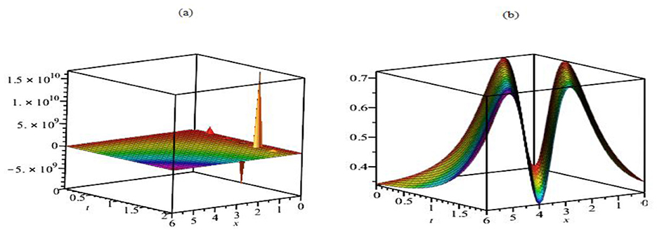
Figure 1. The 3D graphs for the solutions ϕ₁(x, t) (a) and ϕ₈(x, t) (b), where σ = 0, γ = 0.7and α = 1.

The 3D graphs of Figure 2 illustrate how noise strength affects the system's dynamics. In Figure 2a, at noise strength σ → 1, the solution ϕ₁(x, t) appears smooth and planar, indicating that the system's behavior remains stable and uniform across both the x and t domains. In contrast, Figure 2b shows how the solution deviates from this planar structure as the noise strength increases σ > 1. This is evidenced by the emergence of localized spikes and irregularities in ϕ₁(x, t), which reflects the influence of stochastic perturbations. The increased noise introduces randomness into the system, disrupting its deterministic behavior and causing the solution to fluctuate. In a physical context, ϕ₁(x, t) could represent variables such as concentration, temperature, or displacement, while the noise term σ captures external fluctuations like thermal noise, random forcing, or stochastic environmental interactions.

Figure 2

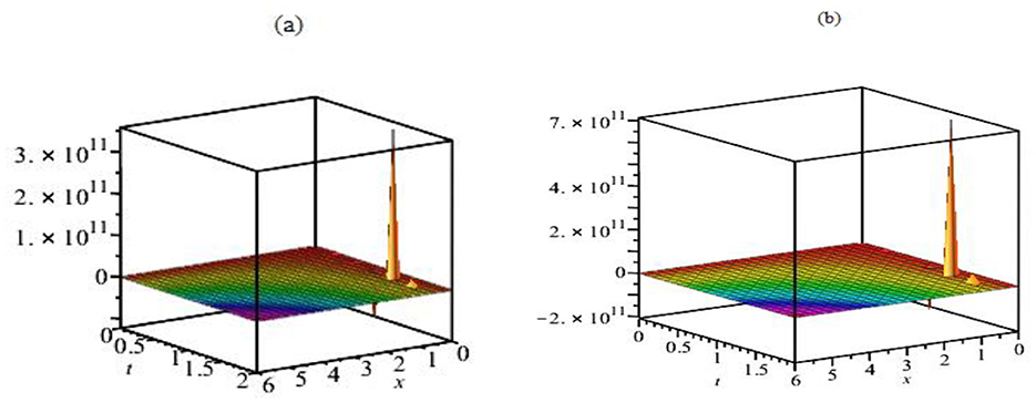
Figure 2. The 3D graphs for the solution ϕ₁(x, t), where γ = 0.7 and α = 1 for σ = 1 (a) and σ = 2 (b).

In Figure 3, the 3D graphs for the solution ϕ₈(x, t), with γ = 0.7 and α = 1 at two different noise strengths σ = 1 and σ = 2 further illustrate how noise influences the system. The noise strength increases from σ = 1 to σ = 2, and the surface transitions from a relatively smooth, planar structure to a more complex, non-planar one. This shift indicates increased noise strength results in more significant fluctuations and distortions, leading to a more chaotic and turbulent surface. These graphs demonstrate how increasing noise strength exacerbates irregularities and disrupts the smoothness and stability of the solution ϕ₈(x, t).

Figure 3

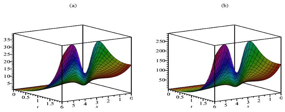
Figure 3. The 3D graphs of the solution ϕ₈(x, t), where γ = 0.7 and α = 1 for σ = 1 (a) and σ = 2 (b).

4.2 The effect of the fractional order

A 3D plots of the solutions ϕ₁(x, t) is presented in Figures 4a–c, where σ = 0, and the parameter curves of the solution are given as follows: (a) α = 1, γ = 0.7, (b) α = 0.8, γ = 0.7 and (c) α = 0.6, γ = 0.7. The impact of the fractional order on the solution behavior is evident as the surface transitions become less planar. Additionally, Figure 4d shows the 2D plot of the solutions ϕ₁(x, t) from Figures 4a–c with the same parameters and x = 1. In the 2D plot, the function value increases with time but decreases with the fractional order, highlighting the sensitivity of the solution to changes in fractional order.

Figure 4

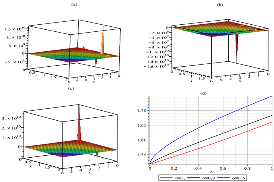
Figure 4. The 3D graphs of the solution ϕ₁(x, t), where γ = 0.7 and σ = 0 for α = 1 (a), α = 0.8 (b) α = 0.6 (c) and x = 1 for (d).

Figure 5 illustrates the impact of the fractional order on the solution behavior of ϕ₈(x, t). The 3D plots of the solutions are shown in Figures 5a–c for the parameter set with σ = 0. In Figure 5a, where α = 1 and γ = 0.7, the solution displays a standard wave-like behavior. As the fractional order α decreases in Figure 5b with α = 0.8 and γ = 0.7, the wave dynamics become more complex, indicating a more substantial influence of the fractional derivative on the solution's behavior, causing the wave to propagate more slowly and with more significant distortion. In Figure 5c, where α = 0.6 and γ = 0.7, the fractional order further reduces the wave speed and introduces more pronounced deviations in the solution, highlighting the increasing effect of fractional behavior on wave propagation. In Figure 5d, 2D plots of the solutions at x = 1 are provided for the same parameter values, where the wave propagation is observed to occur from left to right. As the fractional order decreases, the wave maintains a fixed amplitude, but its propagation rate slows down, with the solution exhibiting a more spread-out, less sharp profile. This behavior can be interpreted as a result of the fractional order modulating the dispersive properties of the system, slowing down wave propagation, and altering its structure.

Figure 5

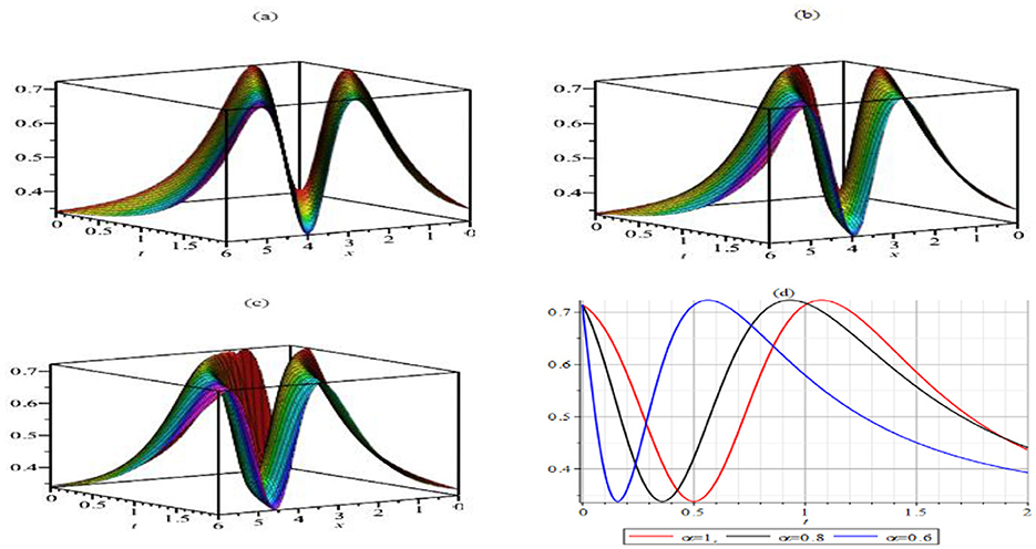
Figure 5. The 3D graphs of the solution ϕ₈(x, t), where γ = 0.7 and σ = 0 for α = 1 (a), α = 0.8 (b) α = 0.6 (c) and x = 1 for (d).

5 Conclusion

This study derived analytical solutions for the STFKS equation using a combination of the Tanh-Coth and He's Semi-Inverse methods with the TMFD technique. The solutions include solitons, waveforms, and singular periodic structures, which are critical for interpreting the behaviors described within the STFKS framework. The findings reveal that as the noise term diminishes, solutions become increasingly planar when the fractional order remains constant. Conversely, in the absence of noise, lower fractional orders lead to more intricate wavefront dynamics, transitioning to less planar forms with consistent amplitude propagation. Graphical representations elucidate these phenomena, emphasizing their physical characteristics. MAPLE software facilitated all computations, demonstrating the methods' efficiency. Notably, the derived solutions align with existing results [e.g., [31, 33]] when the noise term is omitted and the fractional order equals 1. This study underscores the sensitivity of fractional-order systems to noise and fractional order variations. Building on these findings, future research could explore the influence of variable fractional orders and noise intensity in dynamic systems governed by the STFKS equation. Extending these methods to multi-dimensional systems and other fractional differential equations could yield more profound insights into complex physical phenomena.

Data availability statement

The original contributions presented in the study are included in the article/supplementary material, further inquiries can be directed to the corresponding author.

Author contributions

AH: Conceptualization, Methodology, Project administration, Software, Supervision, Writing – review & editing. EG: Conceptualization, Methodology, Writing – review & editing. AA: Conceptualization, Methodology, Writing – review & editing. OH: Writing – review & editing. AS: Writing – original draft, Project administration. MS: Writing – original draft, Visualization. FA: Software, Writing – review & editing. ZM: Writing – review & editing, Validation.

Funding

The author(s) declare that financial support was received for the research and/or publication of this article. This research was funded by Deanship of Scientific Research at Northern Border University, grant number NBU-FFR-2025-1266-03.

Acknowledgments

The authors extend their appreciation to the Deanship of Scientific Research at Northern Border University, Arar, KSA for funding this research work through the project number NBU-FFR-2025-1266-03.

Conflict of interest

The authors declare that the research was conducted without any commercial or financial relationships that could be construed as a potential conflict of interest.

Generative AI statement

The author(s) declare that no Gen AI was used in the creation of this manuscript.

Publisher's note

All claims expressed in this article are solely those of the authors and do not necessarily represent those of their affiliated organizations, or those of the publisher, the editors and the reviewers. Any product that may be evaluated in this article, or claim that may be made by its manufacturer, is not guaranteed or endorsed by the publisher.

References

1. Øksendal B. Stochastic Differential Equation: An Introduction with Applications, 6th ed. Berlin/Heidelberg: Springer (2003).

Google Scholar

2. Khatoon A, Raheem A, Afreen, A. Approximate solutions for neutral stochastic fractional differential equations. Commun Nonl Sci Numer Simul. (2023) 125:107414. doi: 10.1016/j.cnsns.2023.107414

Crossref Full Text | Google Scholar

3. Da Prato G, Tubaro L. Stochastic Partial Differential Equations and Applications. 1st ed. New York: CRC Press (2002). doi: 10.1201/9780203910177

Crossref Full Text | Google Scholar

4. Klebaner FC. Introduction to Stochastic Calculus with Applications. 3rd ed. Singapore: World Scientific Publishing Company (2012). doi: 10.1142/p821

Crossref Full Text | Google Scholar

5. Allen LJS. An Introduction to Stochastic Processes with Applications to Biology. New York: Chapman and Hall/CRC (2010). doi: 10.1201/b12537

Crossref Full Text | Google Scholar

6. Del Moral P, Penev S. Stochastic Processes: From Applications to Theory. New York: Chapman and Hall/CRC (2014).

Google Scholar

7. Alquran M, Jarrah A. Jacobi elliptic function solutions for a two-mode KdV equation. J King Saud Univ. (2019) 31:485–9. doi: 10.1016/j.jksus.2017.06.010

Crossref Full Text | Google Scholar

8. Sahoo S, Saha Ray S. Improved fractional sub-equation method for (3 + 1)-dimensional generalized fractional KdV–Zakharov–Kuznetsov equations. Comput Mathem Applic. (2015) 70:158–66. doi: 10.1016/j.camwa.2015.05.002

Crossref Full Text | Google Scholar

9. Hosseini K, Alizadeh F, Hinçal E, Ilie M, Osman MS. Bilinear Bäcklund transformation, Lax pair, Painlevé integrability, and different wave structures of a 3D generalized KdV equation. Nonlinear Dyn. (2024) 112:18397–411. doi: 10.1007/s11071-024-09944-7

Crossref Full Text | Google Scholar

10. Yildirim A, Gulkanat Y. Analytical approach to fractional Zakharov–Kuznetsov equations by he's homotopy perturbation method. Commun Theor Phys. (2010) 53:2. doi: 10.1088/0253-6102/53/6/02

Crossref Full Text | Google Scholar

11. Hassaballa A, Salih M, Khamis GSM, Gumma E, Adam AMA, Satty A. Analytical solutions of the space–time fractional Kadomtsev–Petviashvili equation using the (G′/G)-expansion method. Front Appl Math Stat. (2024) 10:1379937. doi: 10.3389/fams.2024.1379937

Crossref Full Text | Google Scholar

12. Wang KJ, Shi F, Li S, Xu P. Dynamics of resonant soliton, novel hybrid interaction, complex N-soliton and the abundant wave solutions to the (2 + 1)-dimensional Boussinesq equation. Alex Eng J. (2024) 105:485–95. doi: 10.1016/j.aej.2024.08.015

Crossref Full Text | Google Scholar

13. Fendzi-Donfack E, Kenfack-Jiotsa A. Extended Fan's sub-ODE technique and its application to a fractional nonlinear coupled network including multicomponents — LC blocks. Chaos, Solitons Fractals. (2023) 177:114266. doi: 10.1016/j.chaos.2023.114266

Crossref Full Text | Google Scholar

14. Fendzi-Donfack E, Tala-Tebue E, Inc M, A. Kenfack-Jiotsa A, Nguenang JP, Nana L. Dynamical behaviours and fractional alphabetical-exotic solitons in a coupled nonlinear electrical transmission lattice including wave obliqueness. Opt Quant Electron. (2023) 55:35. doi: 10.1007/s11082-022-04286-3

Crossref Full Text | Google Scholar

15. Fendzi-Donfack E, Nguenang JP, Nana L. On the soliton solutions for an intrinsic fractional discrete nonlinear electrical transmission line. Nonlinear Dyn. (2021) 104:691–704. doi: 10.1007/s11071-021-06300-x

Crossref Full Text | Google Scholar

16. Abdel-Hamid B. An exact solution to the Kuramoto–Sivashinsky equation. Phys Lett A. (1999) 263:338–40. doi: 10.1016/S0375-9601(99)00783-5

Crossref Full Text | Google Scholar

17. Kulkarni S, Takale K, Gaikwad S. Numerical solution of time fractional Kuramoto-Sivashinsky equation by Adomian decomposition method and applications. Malaya J Matematik. (2020) 8:1078–84. doi: 10.26637/MJM0803/0060

Crossref Full Text | Google Scholar

18. Sousa JV, de Oliveira EC. A new truncated M-fractional derivative type unifying some fractional derivative types with classical properties. Int J Anal Appl. (2018) 16:83–96. doi: 10.28924/2291-8639-16-2018-83

Crossref Full Text | Google Scholar

19. Kilbas AA, Srivastava MH Trujillo J. Theory and Applications of Fractional Differential Equations. Amsterdam: Elsevier (2006).

Google Scholar

20. Khalil R, Al Horani M, Yousef A, Sababheh M. A new definition of fractional derivative', J. Comput Appl Math. (2014) 264:65–70. doi: 10.1016/j.cam.2014.01.002

Crossref Full Text | Google Scholar

21. Abdeljawad T. On conformable fractional calculus. J Comput Appl Math. (2015) 279:57–66. doi: 10.1016/j.cam.2014.10.016

Crossref Full Text | Google Scholar

22. Salahshour S, Ahmadian A, Abbasbandy S, Baleanu D. (2018). M-fractional derivative under interval uncertainty: Theory, properties and applications. Chaos Soliton Fract. 117:84–93. doi: 10.1016/j.chaos.2018.10.002

Crossref Full Text | Google Scholar

23. Atangana A, Goufo EFD. Extension of matched asymptotic method to fractional boundary layers problems. Math Probl Eng. (2014) 1:107535. doi: 10.1155/2014/107535

Crossref Full Text | Google Scholar

24. Mohammed WW, Alesemi M, Albosaily S, Iqbal N, El-Morshedy M. The exact solutions of stochastic fractional-space Kuramoto-Sivashinsky equation by using (G′/G)-Expansion method. Mathematics. (2021) 9:2712. doi: 10.3390/math9212712

Crossref Full Text | Google Scholar

25. Wiener N. Differential-space. J Mathem Phys. (1923) 2:131–74. doi: 10.1002/sapm192321131

Crossref Full Text | Google Scholar

26. Mohammed WW, Al-Askar FM, Cesarano C, El-Morshedy M. On the dynamics of solitary waves to a (3 + 1)-dimensional stochastic Boiti–Leon–manna–Pempinelli model in incompressible fluid. Mathematics. (2023) 11:2390. doi: 10.3390/math11102390

Crossref Full Text | Google Scholar

27. Mohammed WW, Cesarano C, Al-Askar FM, El-Morshedy M. Solitary wave solutions for the stochastic fractional-space KdV in the sense of the M-truncated derivative. Mathematics. (2022) 10:4792. doi: 10.3390/math10244792

Crossref Full Text | Google Scholar

28. Haider JA, Alhuthali AMS, Elkotb MA. Exploring novel applications of stochastic differential equations: Unraveling dynamics in plasma physics with the Tanh-Coth method. Results Phys. (2024) 60:107684. doi: 10.1016/j.rinp.2024.107684

Crossref Full Text | Google Scholar

29. Akbari M, Taghizadeh N. Applications of He's variational principle method and modification of truncated expansion method to the coupled Klein–Gordon Zakharov equations. Ain Shams Eng J. (2014) 5:979–83. doi: 10.1016/j.asej.2014.03.012

Crossref Full Text | Google Scholar

30. Malfliet W. Solitary wave solutions of nonlinear wave equations. Am J Phys. (1992) 60:650–4. doi: 10.1119/1.17120

Crossref Full Text | Google Scholar

31. Wazwaz A. Partial Differential Equations and Solitary Waves Theory. Beijing/Berlin: Higher Education Press and Springer-Verlag. (2009). doi: 10.1007/978-3-642-00251-9

Crossref Full Text | Google Scholar

32. He JH. Semi-inverse method of establishing generalized variational principles for fluid mechanics with emphasis on turbomachinery aerodynamics. Int J Turbo Jet-Engines. (1997) 14:23–8. doi: 10.1515/TJJ.1997.14.1.23

Crossref Full Text | Google Scholar

33. Wazzan L. A Modified Tanh—Coth method for solving the general burgers—fisher and the Kuramoto—Sivashinsky equations. Commun Nonl Sci Numer Simul. (2009) 14:2642–52. doi: 10.1016/j.cnsns.2008.08.004

Crossref Full Text | Google Scholar