 Albert Antwi
 Emelia Thembile Kammies
 Lyson Chaka
 Martins Akugbe Arasomwan
- 1Department of Mathematical Sciences, Faculty of Natural and Applied Sciences, Sol Plaatje University, Kimberley, South Africa
- 2Centre for Global Change, Sol Plaatje University, Kimberley, South Africa
- 3Department of Computer Science and Information Technology, Faculty of Natural and Applied Sciences, Sol Plaatje University, Kimberley, South Africa
- 4Department of Statistics, Faculty of Natural and Agricultural Sciences, University of Pretoria, Pretoria, South Africa
Introduction: Accurate price forecasts and the evaluation of some of the factors that affect the prices of grains are crucial for proper planning and food security. Various methods have been designed to model and forecast grain prices and other time-stamped data. However, due to some inherent limitations, some of these models do not produce accurate forecasts or are not easily interpretable. Although dynamic Bayesian generalized additive models (GAMs) offer potential to overcome some of these problems, they do not explicitly model local trends. This may lead to biased fixed effects estimates and forecasts, thus highlighting a significant gap in literature.
Methods: To address this, we propose the use of random intercepts to capture localized trends within the dynamic Bayesian GAM framework to forecast South African wheat and maize prices. Furthermore, we examine the complex underlying relationships of the prices with inflation and rainfall.
Results: Evidence from the study suggests that the proposed method is able to adequately capture the dynamic localized trends consistent with the underlying local trends in the prices. It was observed that the estimated localized variations are significant, which led to improved and efficient fixed-effect parameter estimates. This led to better posterior predictions and forecasts. A comparison to the static trend Bayesian GAMs and the autoregressive integrated moving average (ARMA) models indicates a general superiority of the proposed approach for the posterior predictions and long-term posterior forecasts and has potential for short-term forecasts. The static trend Bayesian GAMs were found to generally outperform the ARMA models in long-term posterior forecasts and also have potential for short-term forecasts. However, for 1-step ahead posterior forecasts, the ARMA models consistently outperformed all the Bayesian models. The study also unveiled a significant direct nonlinear impact of inflation on wheat and maize prices. Although the impacts of rainfall on wheat and maize prices are indirect and nonlinear, only the impact on maize prices is significant.
Discussion: The improved efficiency and forecasts of our proposed method suggest that researchers and practitioners may consider the approach when modelling and forecasting long-term prices of grains, other agricultural commodities, speculative assets and general single-subject time series data exhibiting non-stationarity.
1 Introduction
Climate change has dire consequences for food and water security around the world. In sub-Saharan Africa, food insecurity is exacerbated by a variety of factors, such as slow economic growth, inflation, inaccessibility, price affordability, low investment in irrigation and agricultural research, corruption, and high population growth, among others (1). For example, the mid-year update of the 2022 Global Report on Food Crises by the World Bank (2) indicates that at least an estimated 20% of Africans (140 million) go to bed hungry. The situation is not different in South Africa. A statistically weighted survey conducted by Dlamini et al. (3) in 2021 estimates that the food insecurity rate for South Africa is on par with the average for other African nations. Grains, such as maize and wheat, and products made from them are among the staple foods in South Africa. Fluctuations in the prices of these crops due to climate change, inflation, and other external pressures affect the food security and social stability of the country (4). Therefore, the need to accurately predict the prices of grain futures and how external pressures such as climate change and inflation have become more necessary.
Like many other speculative assets, the prices of grain futures are notoriously difficult to predict due to their inherent nonlinearity and other characteristics such as non-stationarity, trends, and seasonal patterns that vary over time (5). Nonlinearity may be due to the influence of the collective actions or decisions of players such as producers, exporters, importers, processors, handlers, and speculators, etc. which are themselves influenced by nonlinear factors such as opinions, expectations, emotions, sentiments, and unexpected events such as market crashes.
In capturing some of these characteristics associated with the prices of grain futures for accurate modelling and forecasting, literature has predominately focused on the use of traditional time series models such as Autoregressive Integrated Moving Average (ARIMA) and ARIMA generalized autoregressive conditional heteroscedasticity (ARIMA-GARCH) as well as machine learning algorithms such as neural networks [(see 6–10)]. Although these models have been found to be competitive in forecasting prices of agricultural commodities such as corn and other grain prices, they are plagued with some weaknesses that limit their usefulness, especially when assessing the impact of external pressures on the prices. For example, ARIMA models are theoretically appealing and simple to implement; however, the models are inherently linear due to the imposed linearity assumption (11). Consequently, models cannot capture the complex and ever-changing nature of the influencing factors (12) and may also struggle to accommodate extreme events (11).
However, although some machine learning approaches have been found to be competitively better than ARIMA, econometric, and other statistical models (6, 7, 13), they can be time-consuming to train and often require a large amount of data to properly train the models (14). Furthermore, unlike many statistical and econometric models, traditional machine learning models are not inherently built to simultaneously model causal relationships in addition to forecasting and predictions (15). It should be noted that there is growing literature focusing on integrating casual modelling into machine learning algorithms (16–19). However, this new class of models also comes with limitations in terms of casual interpretations. For example, many casual machine learning models assume casual relationships that do not change over time and are inconsistent with time series data. Although limited attempts have been made to address this problem (16–19), they often yield computationally intractable solutions as the number of features increases; especially when computing Shapley values. Moreover, the incorporation of plausibility and actionability constraints into the models also results in NP-hard1 or NP-complete problems when solving integer-based variable problems, neural network problems, or problems involving quadratic objectives and constraints (20, 21).
Bayesian generalized additive models (Bayesian GAMs) provide an alternative approach to overcome some of the limitations of econometric and machine learning models. They provide a flexible nonparametric framework that allows the use of splines to capture complex patterns and nonlinearity within the time series data (14). The framework accommodates fully parametric and semiparametric specifications; thus, Bayesian GAMs can build on the strengths of parametric and nonparametric models to improve forecasts (14). Furthermore, the Bayesian GAMs can accommodate prior beliefs about the population parameters in the modelling process and are also well suited for small sample sizes due to their ability to stabilize the estimated parameters (22). The Bayesian GAMS have gained traction in areas such crop production (23), climate change and human health (24), electric load forecasting under extreme weather conditions (25), agricultural commodity prices (26) and general statistical modelling (27) due to their ability to model complex nonlinear relationships. A recent variation of the Bayesian GAM, the dynamic GAM (DGAM), has also been proposed by Clark and Wells (28) to model discrete ecological time series data. Nonstationary time-series data for single subjects are not considered as cross-sectional data because they do not involve many subjects observed at a single point or period in time. Therefore, the use of Bayesian GAMs in modelling and forecasting nonstationary time series data such as agricultural commodity yield and prices (23, 26), ecological data (28), among others, do not isolate the local trends from the global or the overall trend, thus by default they are assumed to be static. However, time aggregation effects at both micro time frames (e.g., daily) and macro time frames (e.g., monthly or annually) can obscure heterogeneity in local trend fluctuations (29) which can potentially lead to biased fixed effect estimates and less accurate predictions and forecasts if left uncounted for in the modelling process.
To address this problem, we propose the incorporation of dynamic local trends into the dynamic Bayesian GAM framework (hereafter called Dynamic Local Trend Bayesian GAM or simply Dynamic Trend model) to account for the obscured heterogeneity in local trend fluctuations in South African maize and wheat prices to improve efficiency of fixed parameter estimates and the overall posterior forecasts. In addition to this, the study explores the non-linear impacts of inflation and rainfall on prices to understand how changes in these exogenous factors affect prices. By allowing the local trends and the uncertainties surrounding them to dynamically evolve over time, the proposed Dynamic Local Trend Bayesian GAM is expected to offer more efficient estimates and improved posterior forecasts in comparison to competing models, thus allowing farmers, government, and other stakeholders to make timely and informed decisions to ensure food security, accessibility, and affordability.
The rest of the article is organized as follows: Section 2 is a detailed review of the literature. Section 3 gives a brief overview of the data used, the analytical methods, and the model evaluation approaches applied. The empirical results and discussion thereof are given in Section 4, while the conclusions and recommendations are given in Section 5.
2 Literature review
The dynamic Bayesian GAM was introduced recently by Clark and Wells (28) to model complex ecological time series data. However, although it offers promising applications in the prediction of grain futures, its use has not received much attention. The literature has primarily focused on the use of traditional time series models such as ARIMA and SARIMA to forecast grain prices and the price of other agricultural commodities, as well as to assess the impact of external factors such as inflation and climate change on prices. Although these models are simple and theoretically appealing, their simplicity imposes structural limitations on them, which makes them unable to model complex relationships. Despite their weaknesses, traditional time series models have been found to be useful in forecasting prices of agricultural commodities such as corn and other grain prices.
One of such studies was conducted by Diop and Kamdem (8). In this study, the authors used a univariate time-frequency decomposition-based approach to choose a seasonal autoregressive integrated moving average (SARIMA) model to predict monthly prices for specific agricultural futures. They focused on identifying a SARIMA model that is suitable for explaining the rise in the indexes of agricultural prices and then using the resulting model to generate forecasts. The data used was divided into two periods: January 1980 to December 2016 (37 years with 444 observations) and the year 2017. It was found that the complete seasonal ARIMA model SARIMA (p, d, q) (P, D, Q) 12 was superior to forecasting agricultural time series data compared to other SARIMA models.
Another study by Albuquerquemello et al. (9) compared the precision of various macroeconomic models used in financial literature from 1995 to 2017. Using multivariate transition regime models, which account for structural breaks, the model was found to provide better forecasts for corn prices. The study suggested that the best models should consider not only the structure of the corn market but also financial and macroeconomic fundamentals, as well as transition regimes and non-linear trends, such as threshold autoregressive models. In the same year, Zhou used univariate ARIMA to forecast monthly corn prices data for 23 months from April 2019 to February 2021. From the analysis, a forecast was made for the price of corn in March 2021 in China. After comparing the experimental results with the actual price, the model showed a good fit and accurate predictions for corn prices in China (30).
Furthermore, Saxena and Mhohelo (10) assessed the effectiveness of ARIMA models in forecasting maize prices in the Gairo, Manyoni, and Singida markets in Tanzania using historical monthly data from January 2009 to May 2019. Before the data was used in fitting the ARIMA models, the Augmented Dickey-Fuller test was used to assess the stationarity of the time series while autocorrelation and partial autocorrelation plots were used to identify the appropriate orders for the autoregressive and moving averages of the ARIMA model. After fitting the models, the mean squared error, mean absolute error, mean percentage error, and mean absolute percentage error were used to evaluate forecast performance. Evidence from the study indicates that ARIMA (1, 1, 4),2 ARIMA (2, 1, 3) and ARIMA (2, 2, 3) were selected as the best fitted models for the maize prices from the Gairo, Manyoni and Singida markets, respectively. These models have lower information criteria and MAPE values compared to alternative models. From the forecast, the authors concluded an increasing price outlook for maize prices within these markets over the period June 2018 and May 2019, highlighting the importance of accurate forecasting to help producers and consumers make informed decisions when buying and selling maize crops in Tanzania.
On the use of machine learning models, the superiority over traditional time series models is clearly visible in literature despite their inability to explain the evolution of the underlying relationships among the target and the features. For example, Jin and Xu (13) emphasized that accurate price predictions of agricultural products are crucial for farmers, traders, and policymakers to make informed decisions. However, they argue that the traditional forecasting methods are limited in capturing nonlinear patterns and seasonal variations, thus they explore the application of neural networks in forecasting prices of green beans to improve the forecasts. In this quest, they employed neural network, support vector machine, and regression tree models and then evaluated their performance in comparison to traditional models such as autoregressive (AR), AR-GARCH models, and the no-change model. The data consist of the weekly price index of the Chinese market over from January 1, 2010, to January 3, 2020. Although the results indicate the superiority of the neural network model in forecasting green beans index prices in comparison to the other machine learning and econometric models, the econometric models turn out to perform badly in comparison to the other machine learning models such as the support vector machine and regression tree model, but it performed better than the no-change model.
In another study, Brignoli et al. (6) evaluated the performance of the Long Short-Term Memory Recurrent Neural Networks (LSTM-RNNs) model in comparison to econometric models such as ARIMA, the vector autoregressive and vector error correction model in forecasting corn futures prices. In addition to corn futures prices, the data set included 12 other external time series variables such as the dollar and gasoline prices, among others. The data set consisted of a total of 5,174 observations for each series that spanned January 2000 to June 2020. The analysis of the study suggests that the LSTM-RNNs model exhibits superiority in forecasting corn futures prices over all horizons, particularly for long periods. Furthermore, it was observed that the LSTM-RNN model was able to automatically accommodate structural breaks in the modelling process, which contributed to its superior performance. Although the LSTM-RNNs performed consistently better than the econometric models over various horizons, it was found that the model has difficulty handling seasonality and trend components and may require specific transformations or constructions when incorporating the components.
Wang et al. (7) also applied a hybrid of LSTM and a convolutional neural network (LSTMCNN) to forecast grain prices of commodities in the United States of America. The data included weekly grain prices such as oat, corn, soybean, and wheat and 14 characteristics that include macroeconomic variables and weather variables such as snow water equivalent, snowfall, and snow depth from 1990 to 2021. The performance of the LSTMCNN model was then compared with that of the traditional ARIMA and the standalone LSTM and CNN model using the mean squared error evaluation metric. It was observed that across all forecast horizons (5, 10, 15 and 20 weeks), the hybrid LSTMCNN model consistently outperforms the ARIMA and the standalone LSTM and CNN models. The ARIMA model was also outperformed by the LSTM and CNN models. These results confirm the superiority of the machine learning model over the classical ARIMA model.
In summary, the literature review shows a shift towards advanced techniques such as machine learning models and sophisticated econometric models such as AR-GARCH in forecasting agricultural commodity prices using historical price data and relevant features. Although the superiority of machine learning models over econometric models has been established due to their flexibility in modelling the underlying complex structure of agricultural commodity prices; they lack interpretability (31). Because of this, it is difficult to understand the evolution of the underlying relationship among agricultural commodity prices and predictors. Nonparametric approaches such as the Bayesian GAM provide an alternative framework for flexibility, robustness and interpretability while improving performance. These provide Bayesian GAM models with competitive advantage over machine learning algorithms; thus the framework is proposed in this study forecasting the grain prices.
3 Data and methodology
3.1 Data
The paper uses monthly historical data of wheat and white maize prices from RSA SAFEX Domestic Future, which was accessed from www.sagis.org.za/safex_historic.html. Data on consumer price index (inflation) was obtained from www.investing.com while precipitation index (rainfall) was obtained from the Giovanni Earth data website.3 The sample period spans from January 2000 to March 2024. The choice of the sample period was solely based on the availability of data for all variables, while the choice of inflation and rainfall is also based on their notable impact on grain prices and their ability to improve price forecasts.
3.2 Dynamic Bayesian generalized additive model
The development of generalized additive models GAMs in estimating smooth nonlinear relationships between predictors and response variables through a backfitting algorithm was pioneered by Hastie and Tibshirani (32) as an extension of generalized linear models (33) to allow non-parametric smooth functions (such as splines) instead of fixed linear terms. The concept received subsequent developments and refinements, particularly in the context of using penalty terms to control the overfitting of smooth functions (34) and the combination and flexibility of nonparametric regression with mixed models (35), leading to the development of generalized additive mixed models (GAMMs). GAMMs are capable of capturing nonlinear effects while accounting for random effects in correlated observations within clusters. In addition, Solonen and Staboulis (36) introduced the Bayesian generalized additive models which incorporate prior distributions and posterior inference to provide full probabilistic uncertainty quantification while allowing flexible, non-linear relationships between predictors and a response variable. Recently Clark and Wells (28) introduced a dynamic Bayesian GAM to model complex discrete ecological time series data.
However, the model allows the exogenous factors to evolve over time as either a random walk with constant drift or as an autoregressive process, and thus it does not inherently or explicitly account for variations in the local trend. This may lead to several problems including biased fixed effect estimates, misleading inference about trends or temporal effects, and poor model fitness and predictive performance. The unmodeled heterogeneity across the time series periods (quarters, years, etc.) may confound the temporal effects thus leading to apparent trends or fixed effects, which may otherwise be due to the presence of time heterogeneity. To address this, we propose the incorporation of dynamic temporal trends into the dynamic Bayesian GAM framework to account for the observed fluctuations in the local trends in grain futures prices, as indicated below.
Consider a time series and a set of predictors , then the dynamic generalized additive model of Solonen and Staboulis (36) is defined in Equation 1 as follows:
Here denotes the overall or global intercept (trend), are the basis functions for predictor i with coefficients , is the dynamic part which captures time varying local deviation in the time series and is the error component. The prior distribution of is assumed to follow the skewed t-distribution, to account of heavy-tails and skewness commonly observed in the prices of speculative assets, thus . The skewed t-distribution is defined in Equation 2 below:
The parameters are the location, scale and shape parameters respectively, and is the Gamma function. The scale parameter specifically accounts for the uncertainty in the model; the shape parameter controls the skewness in the data, while the location parameter represents the mean. It should be emphasized that . The dynamic component of the model captures the underlying temporal dependence. The component is assumed to follow an ARMA process which is defined in Equation 3:
where p and q are integers, and are real coefficients, and are, respectively, the autoregressive and the moving average terms. To incorporate temporal variations in the local trend to account for obscured heterogeneity due to time aggregation effect, the global intercept is reparametrized as a sum of the fixed effect and the random effects or local trends and as indicated in Equation 4.
The intercept of the local trend measures group-specific deviations from the global trend. It accounts for heterogeneity at the group level such as different years, where unique events (such as pandemics, food shortages, geopolitical risks, etc.) might cause certain years to have systematically higher or lower localized trends than what the global trend predicts. Therefore, the random intercepts capture group-level shifts, which allow the model to isolate group variations from the global trend, especially in the presence of localized influences. On the other hand, the random slope captures how the effect of time varies across groups like quarters or years. This allows the model to distinguish between global trends and group-specific time trends. By doing so, it isolates the specific contribution of trends from each group to the overall trend, thus highlighting whether some groups have stronger or weaker temporal changes.
3.3 Choice of splines
The dynamic additive model formulated in Equation 1 requires the specification of the basis function to allow the model to fit the underlying non-linear structure. There are several types for these basis functions which include the B-splines, cubic spline, penalized splines and adaptive splines among others (37). However, the choice of an appropriate function depends on the nature of the underlying relationship between the variable of interest (outcome or target) and the external variables. A look at the scatter plots in Figure 1 clearly shows that cubic splines are appropriate for the data. This is because the observed relationship between inflation and the prices of maize and wheat is a cubic function. On the other hand, although the observed relationship between rainfall and maize and wheat prices does not appear to show any clear patterns, cubic splines may also be appropriate. For these reasons, cubic splines are used in modelling the underlying complex dynamics among the variables in the data.
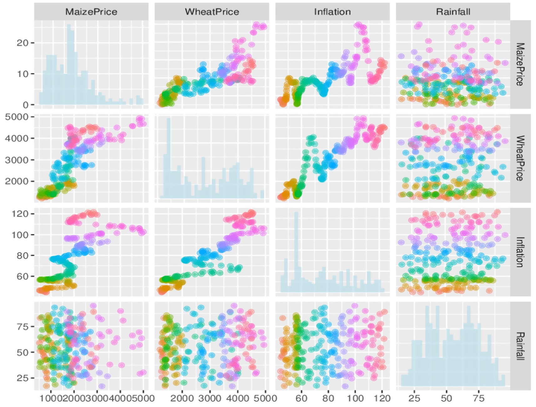
Figure 1. Scatter plots indicating the nature of relationships among the variables.
3.4 Parameter estimation via the Markov chain Monte Carlo algorithm
Parameter estimation of the Bayesian generalized additive models often involve sampling from probability distributions whose densities are intractable, thus a common approach to tackle this problem is through the use of parameter estimation via the Markov Chain Monte Carlo (MCMC) algorithm (38). The MCMC algorithm requires the drawing of sequential random samples (called Markov chains) from a prior distribution where each chain state is dependent only on the previous chain state. The process continues until the chains converge to the desired distribution. After convergence, selected increments of the states of the chain are then used to construct the parameters of interest, and the necessary inferences are then made on the estimated parameters (38).
The most common MCMC algorithms used included Metropolis-Hastings, Gibbs sampling, and Hamiltonian Monte Carlo sampling (39). The use of each of these methods depends on the task at hand. For example, the Metropolis-Hastings algorithm is used when the parameters at hand do not allow for easy sampling. Gibbs Sampling is used when the full conditional distribution can be directly derived. On the other hand, Hamiltonian Monte Carlo is used for continuous distributions, as is the case in this study. The Hamiltonian Monte Carlo leverages on the gradients of the log-posterior and it is built on theoretical foundations of differential geometry; thus, it is suited for high-dimensional data, and has proven to be completely well even for complex problems (40).
The estimation algorithm starts with defining the likelihood function. Consider the parameter space . Given the observed data conditioned on , the likelihood of the observed data can be expressed as in Equation 5:
From the likelihood function, the posterior distribution of the model parameters given the observed data is therefore derived using the Bayes theorem which can be simplified as shown in Equation 6:
where represent the distribution while represents the prior distributions. The following priors were imposed on the parameters of the estimated models. The flat priors (noninformative) were used for the fixed parameters of the autoregressive and the regression parameters (rainfall and inflation) since we have no prior beliefs about these parameters. The weakly student-t informative priors were used for the global intercept, standard deviations of the spline parameters (inflation and rainfall), the residual standard deviation (scale parameter associated with the residual), and the random effects (random intercepts and random slopes). For each of the parameters, the estimated sample degrees of freedom, location, and scale were used as the input for the student-t priors. Specifically, student-t (3, 2775.6, 1628.2) and student-t (3, 1773, 927.9) are the respective priors for the global trends for the wheat and the maize data. The student-t (3, 0, 1628.2) and student-t (3, 0, 927.9) priors were also used for the standard deviations of the spline parameters, the residual standard deviation and the random effects for the wheat and maize prices, respectively.
The shape parameter associated with the residuals was also modelled by the informative gamma prior indicated by gamma (2, 0.1). The choice of this prior is supported by an empirical study (41) that found that the Gamma (2, 0.1) prior performs well in practice. The prior balances flexibility and informativeness of the degrees of freedom parameter by modelling a wide range of shapes, which is enough to guide the estimation process without being overly restrictive. The prior also has a mean of 20 and a variance of 200, which provides a reasonable belief for the estimation of the degrees-of-freedom parameter, thus ensuring convergence and stability. The flexible but non-informative Lewandowski–Kurowicka–Joe distribution (42) prior was used for the correlation matrix constructed from the random intercepts and slope within the hierarchical trend model formulation. This prior is more useful in situations where no strong prior knowledge about the correlation matrix exists, as is the case here. The MCMC algorithm starts by initializing all the parameters and then repeatedly iterating all the parameters for a predefined number of times until all the chains converge as discussed below.
Step 1: Initialization
• Initialize the parameters space to some constants obtained from the individual priors.
Step 2: Iteration
• For each iteration steps , generate a new proposal sampled from the full conditional distribution in Equation 7:
where represents the parameter and denotes the remaining parameters after removing the parameter. For example, given the fixed parameter , is sampled from the student-t distribution indicated in Equation 8:
Step 3: Acceptance probability
• Compute the Metropolis-hastings acceptance probability (α) using Equation 9:
where represents the current value of the parameter at iteration of the MCMC chain.
Step 4: Acceptance decision
• Draw a random number from a uniform distribution . If accept otherwise reject and retain the current value.
Step 5: Repeat iterations
• After accepting or rejecting the new proposal, proceed to the next iteration at step 2 and repeat the process until all the iterations have been exhausted.
Step 6: Iteration for the remaining parameters
• Repeat the steps 2 through to 5 for each of the remaining parameters until all the iterations have been exhausted.
Step 7: Convergence diagnostics for chains
• Using methods such as Trace Plots, Effective Sample Size (ESS) and Gelman-Rubin Statistic ( ), convergence of the estimated parameters cam be assessed. The trace plots visualise the MCMC chains for stationarity by superimposing the posterior distribution of the chains on the distributions of random draws. A clear near complete overlapping of the two plots coupled with an effective Sample Size >1,000 and across multiple chains indicate suggest a good mixing chains, hence converging chains which can be used for reliable inference. On the other hand, if the chains are not mixing well or converging, the model may need to be re-parameterized and the estimation process repeated. Non-convergence chains may also be due to outliers; in which case the problematic observation should be removed, and the iterations are then repeated.
Once convergence has been reached, the posterior forecasts for new data can be obtained from the posterior samples using Equation 10.
After the parameters of the Bayesian GAMs have been fitted using the MCMC algorithm, a large number of posterior samples from all the model parameters are generated to construct a predictive distribution. The algorithm then draws samples from the predictive distribution at each forecast step to generate a posterior forecast that accounts for the uncertainty of the parameters, residual variation, and random effects through incorporation of the posterior standard deviations to construct the credible intervals and other necessary estimates. By capturing the combined uncertainty in the data, model parameters, and their relationships through predictive draws, the model can capture the overall uncertainty in the posterior forecasts.
4 Empirical results
4.1 Preliminary data analysis
The preliminary data analysis aims to understand the distribution and the underlying patterns and structure the target variables (maize and wheat prices) so that they are appropriately incorporated into the modelling process. For this reason, we report and discuss descriptive statistics, test for normality, and then assess the autocorrelation structure of the data. Table 1 provides descriptive statistics, while Figure 2 displays quantile plots. In Figure 3, autocorrelation graphs are reported, while Figure 4 shows seasonal decomposition graphs.
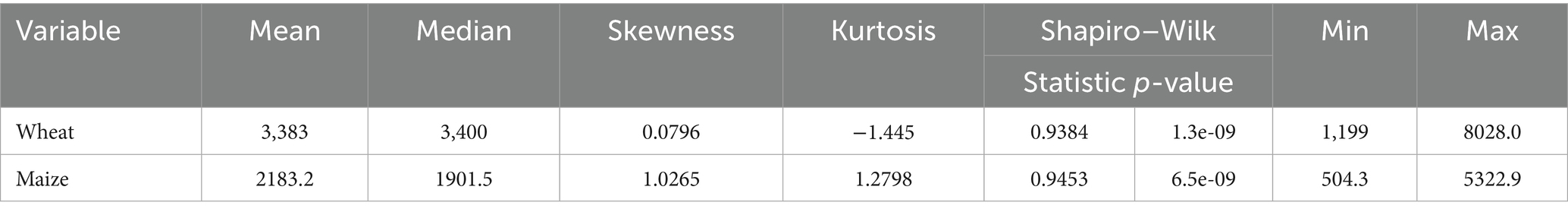
Table 1. Descriptive statistics of wheat and white maize prices.
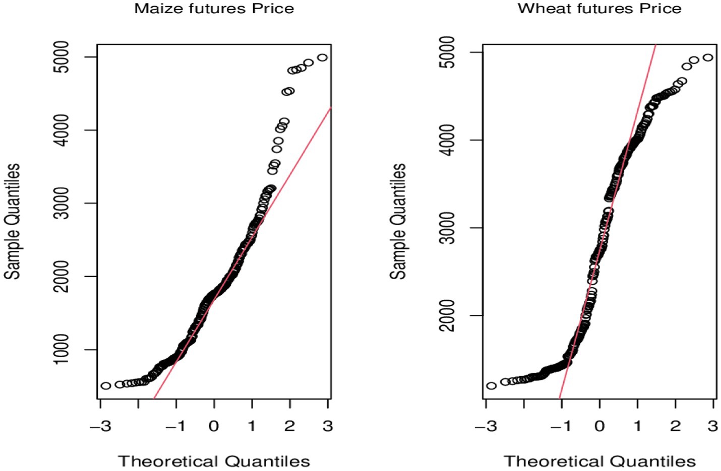
Figure 2. QQ plots for wheat and maize prices.
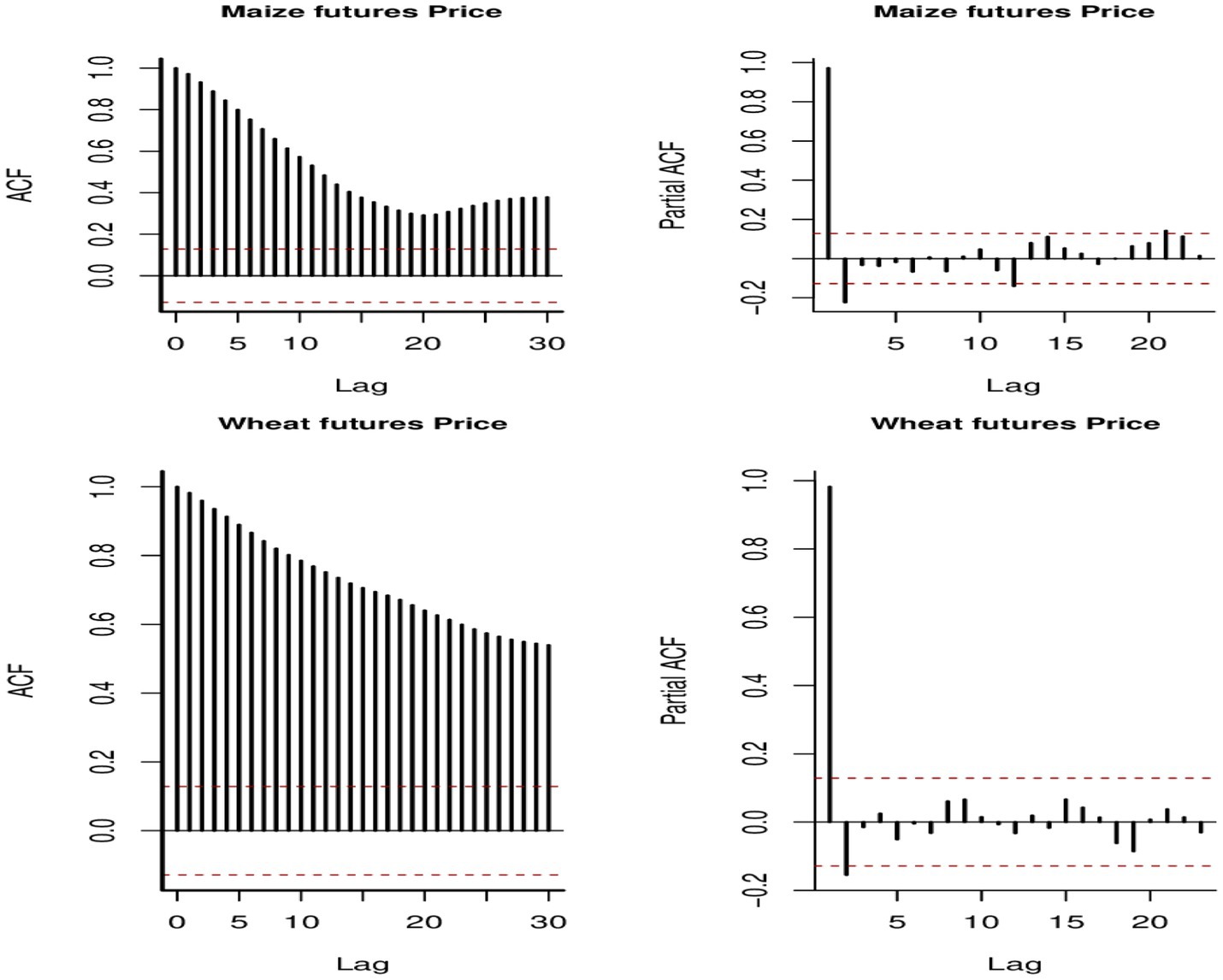
Figure 3. ACF and PACF plots for wheat and maize prices.
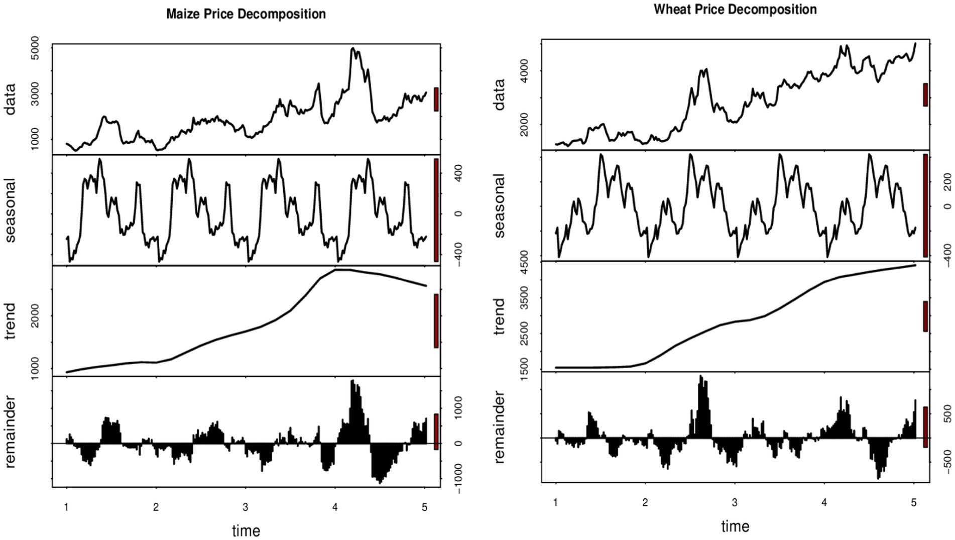
Figure 4. Seasonal decomposition plots for wheat and maize prices.
In Table 1, the respective skewness values for wheat and maize prices are 0.0796 and 1.0265, suggesting that both prices are positively skewed. The positive skewness of the prices is confirmed by the minimum and maximum values, which are all positive. Furthermore, a look at the kurtosis values indicates that both prices are more peaked than the normal distribution, but the tail of the wheat price is flatter than the maize price due to its negative value. These observations indicate that the wheat price data is platykurtic (lighter tails and a flatter peak), while the maize price data is leptokurtic (heavier tails and a sharper peak), suggesting that prices are not normally distributed. The observations are confirmed by the test results from the Shapiro–Wilk normality test and the QQ plots since the p-values of the Shapiro–Wilk test are less than 0.05 and the empirical quantiles deviate significantly from the theoretical quantile (straight line) as shown in the QQ plots. These observations suggest the use of a heavy-tailed distribution, such as the skewed student t-distributions, to model the prices.
Price data are time series since they consist of observations that are recorded at regular intervals over time, and thus the data need to be checked for characteristics of time series such as seasonality and autocorrelations so that they can be accommodated in the modelling framework if they are present. The autocorrelation function (ACF) and partial autocorrelation function (PACF) plots are therefore important for analyzing the time-series data to understand the relationships between the observations at different time lags. Figure 3 shows the ACF and PACF plots for wheat and maize prices, which are important for identifying the AR and MA structures present in the data. When ACF gradually decreases and PACF cuts off sharply, it suggests an AR model. On the contrary, when ACF has a sharp cutoff point and PACF has gradual decay, it indicates an MA model. The plot suggests an AR (2) structure for wheat and maize prices data since the ACF plots gradually decrease and the PACF plots indicate two prominent spikes outside the 5% confidence bounds (the dotted lines), respectively. Maize and wheat are seasonal crops; therefore, it is appropriate to assess the presence or absence of seasonality in the prices of the crops. A look at the seasonal decomposition plots suggests the absence of seasonality in the data and thus no need to incorporate seasonality into the models. However, the plot indicates a dynamic trend that needs to be accommodated in the models.
4.2 Diagnostics of the estimated Bayesian dynamic GAMs
Techniques such as posterior probability plot, Rhat, tail effective sample size (ESS), the bulk ESS, and the Leave-One-Out (LOO) cross-validation method are used in assessing the fitness of the estimated models. The posterior distribution plot is a plot of the posterior distribution superimposed on the distributions of random draws. The Rhat model is evaluated by comparing the variation within the chains with the overlap between the chains. The tail ESS estimates the number of independent samples obtained from the posterior distribution, which corresponds to the number of independent samples that have the same estimation power as the n autocorrelated samples (43). On the other hand, the bulk ESS indicates the number of samples the sampler took from the denser part of the distribution, while the tail ESS reflects the time spent in the tails of the distribution. For a well-fitted model, both Bulk ESS and Tail ESS should exceed 1,000 and the Rhat values should be greater than 1 (44). Furthermore, the posterior distribution plot should overlap with the distribution plots of random draws. The Rhat assesses the convergence of the model by comparing the variation within the chains to the overlap between chains. The LOO method assesses the predictive ability of posterior distributions. If all the Pareto estimates from the LOO estimates are less than 0.07, a model is considered to have good predictive ability. However, if any of the pareto estimates is greater than 0.7, it is an indication that the importance sampling may be unstable, suggesting that the predictive accuracy may be inaccurate or misleading (over-fitting or under-fitting), which may be due to the presence of outliers in the data. The results of the diagnostic tests and graphs are reported in Figures 5a,b, Tables 2, 3.
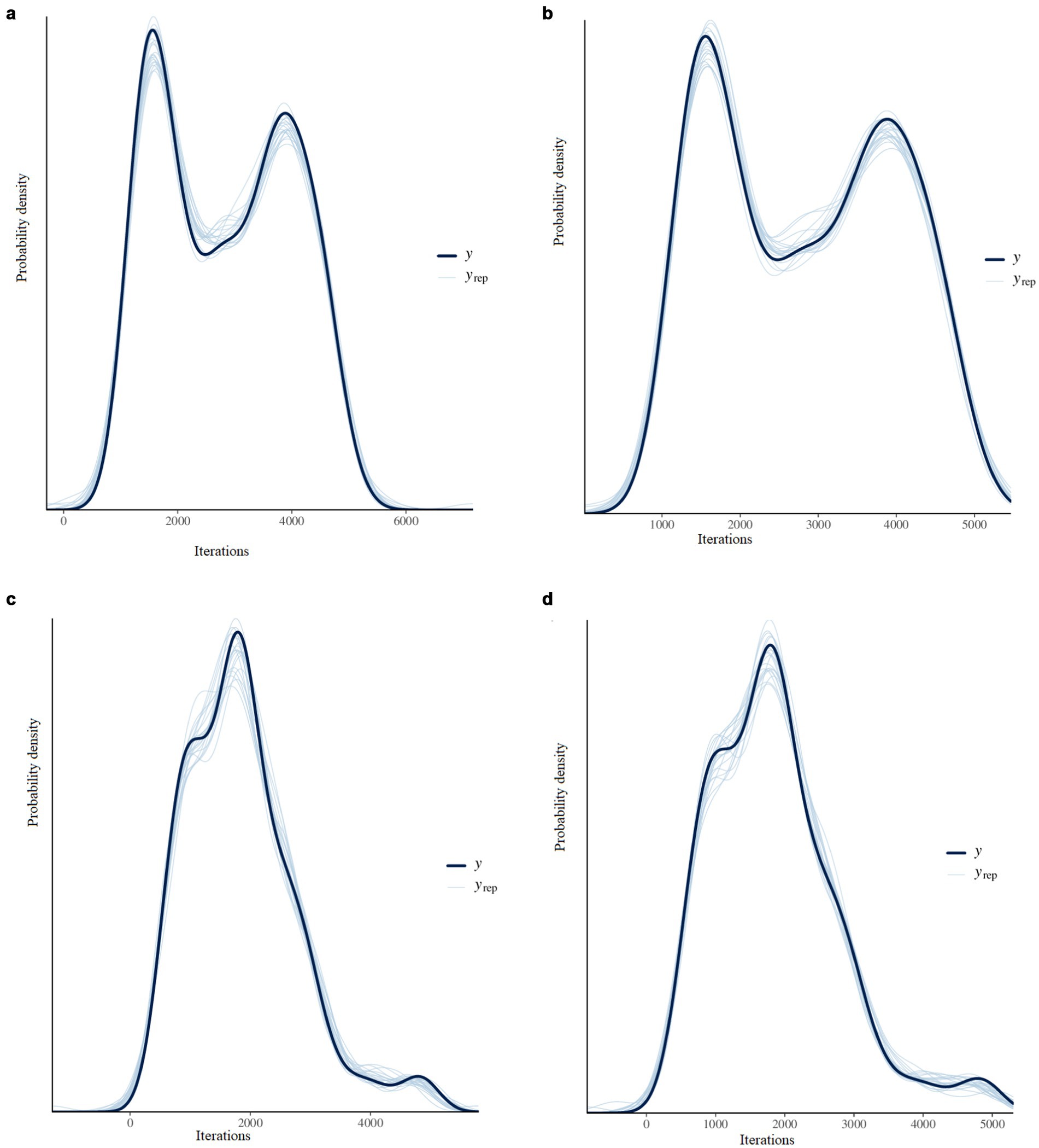
Figure 5. (a) Posterior distribution plots for the wheat price data from the dynamic local trend model. (b) Posterior distribution plots for the wheat price data from the static trend model. (c) Posterior distribution plots for the maize price data from the dynamic local trend model. (d) Posterior distribution plots for the maize price data from the static trend model.
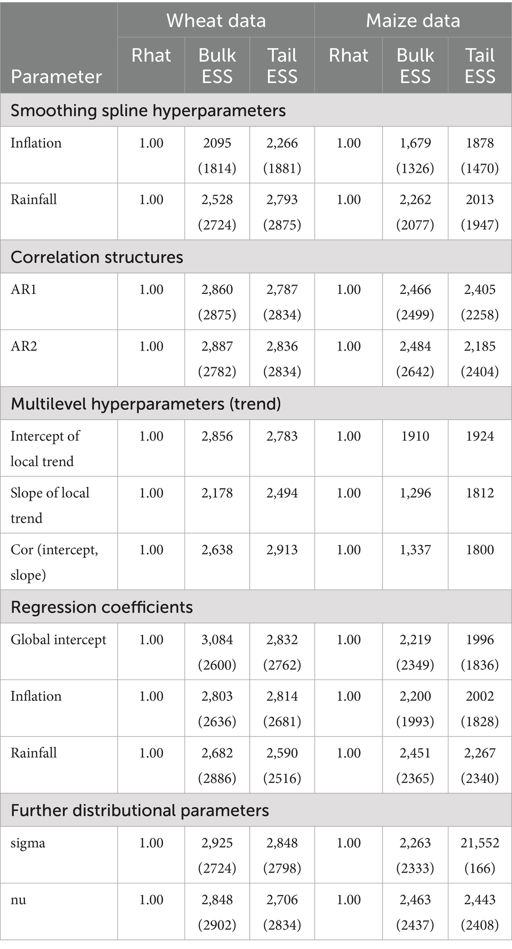
Table 2. Dynamic Bayesian GAM convergence estimates for the models for wheat prices.
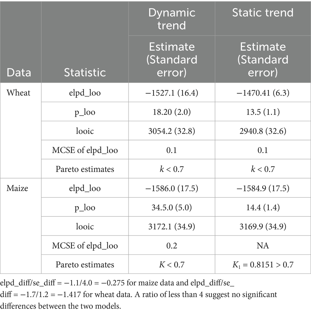
Table 3. Leave-one-out (LOO) cross-validation tests.
From the posterior probability plots in Figures 5a–d, the thin light blue lines represent the distribution of 20 random draws, while the dark blue line represents the posterior distribution of the prices. From the plots, it is observed that the thin light blue lines almost overlap with the dark blue line. The Rhat values reported in Table 2 are all less than 1 for all parameters in each of the models. Furthermore, the bulk ESS and tail ESS values exceed 1,000 for all models. Finally, with the exception of the static trend model for the maize data, the reported pareto estimates in Table 3 for all the observations in the respective models are less than 0.7. These results suggest that all of the estimated Bayesian models fit well with the respective data except for the static trend model for the maize data.
4.3 Assessing efficiency of estimated parameters of the Bayesian GAMs
Our proposed methodology requires the trend parameters, the intercept and the slope to vary over time, which adds more complexity and flexibility to the model. However, it is important to assess whether the added complexity and flexibility yield more efficient parameter estimates. The evaluation is done by comparing the posterior standard deviation (denoted as estimated error) and the credible intervals (denoted as L-95% CI and U-95% CI) of the proposed dynamic local trend model to the static version. A smaller posterior standard deviation accompanied by shorter credible intervals indicates less uncertainty about the parameter estimates, which may indicate a more efficient parameters. On the other hand, larger posterior standard deviations with wider credible intervals may suggest less efficient parameter estimates.
The results are presented in Tables 4, 5. Observations from Table 4 indicate that the dynamic local trend model generally yields a reduced posterior standard deviation and shorter credible intervals compared to the statistic version. Exceptions were observed, however, with the AR (2) parameter, the regression coefficient for inflation, and the nu-distributional parameter where both models yielded approximately the same posterior standard deviations and credible intervals, or the static trend model yielded better estimates. In the case of the maize data, as indicated in Table 5, the static trend model has its nu-distributional parameter having a lower posterior standard deviation and a shorter credible interval than the dynamic local trend model. Furthermore, the static trend model has approximately the same posterior standard deviation as the dynamic trend model for the AR (2) parameter and the smoothing spline hyperparameter for inflation; however, the dynamic local trend model has a shorter credible interval for these parameters. For all other parameters, the dynamic local trend model has lower posterior standard deviation and shorter credible intervals. The observed lower posterior standard deviation and shorter credible intervals associated with the dynamic local trend models suggest that the added complexity and flexibility generally produced more efficient parameter estimates because the models are able to capture the underlying structures of the maize and wheat prices accurately.
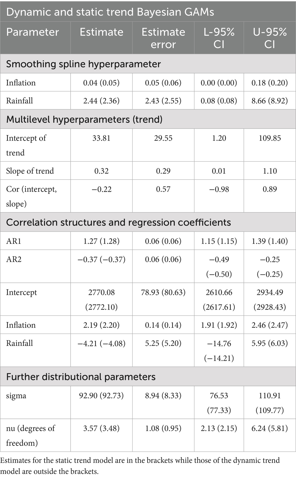
Table 4. Estimated parameters for dynamic and static trend Bayesian GAMs for wheat prices.
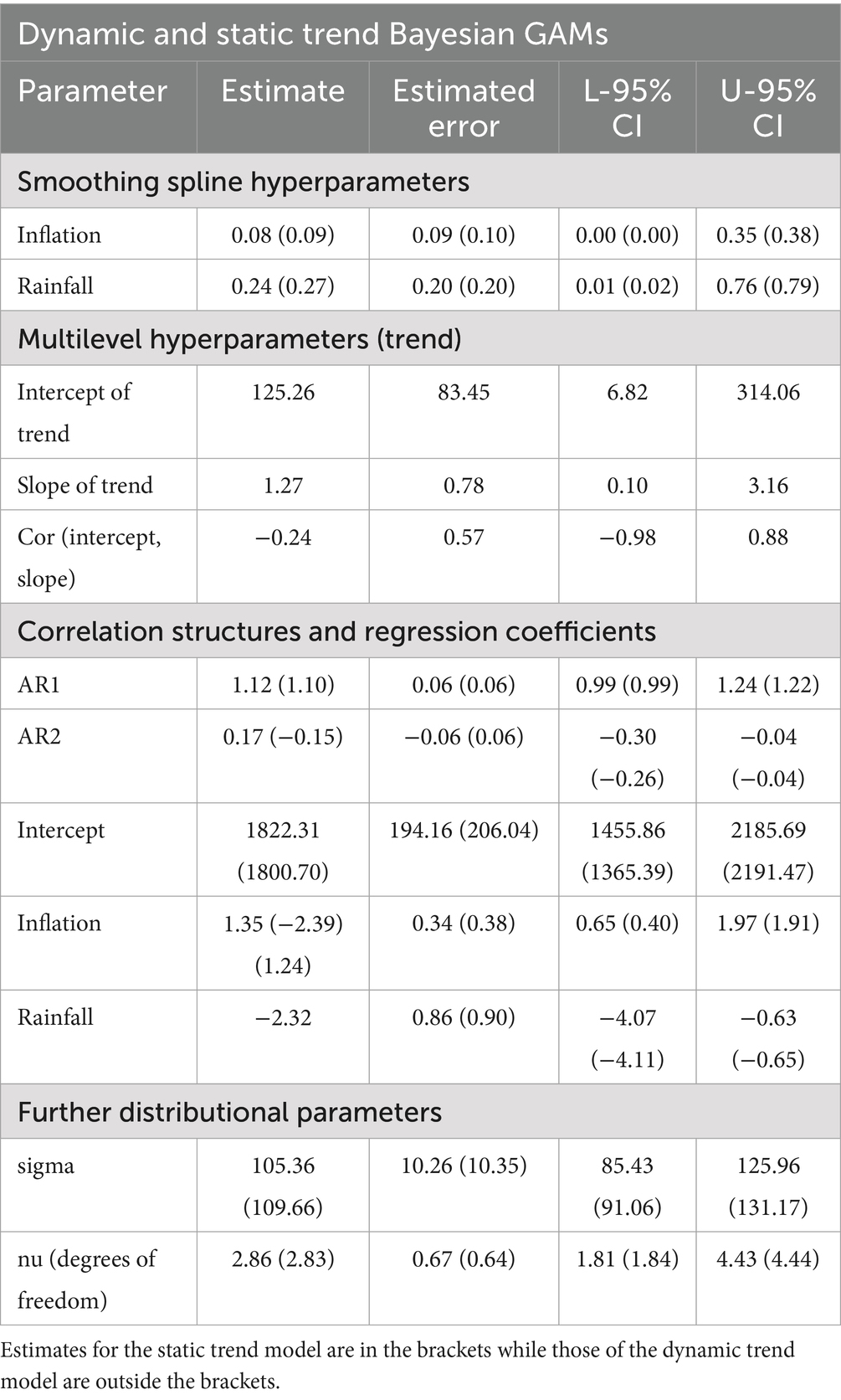
Table 5. Estimated parameters for dynamic and static trend Bayesian GAMs for maize prices.
4.4 Model performance comparisons
The observed efficiency of the dynamic local trend model in comparison to the static trend model is expected to translate into more accurate predictions and forecasts, thus the need to assess the posterior predictive and forecast performances of the dynamic local model. In this exercise, a comparison is made with the static trend model. The ARIMA models are commonly used in forecasting grain prices, and thus we also compare the performances of trend models with the ARIMA models. For fair comparisons, the same autoregression orders and predictors were used in estimating all models. We report the in-sample performance metrics and the out-of-sample performance metrics for short-term (1, 3 and 7 months ahead) and long-term (36 and 48 months ahead). The metrics used include the mean absolute percentage error (MAPE), the mean absolute error (MAE), and the root mean square error (RMSE). The results are reported in Table 6.
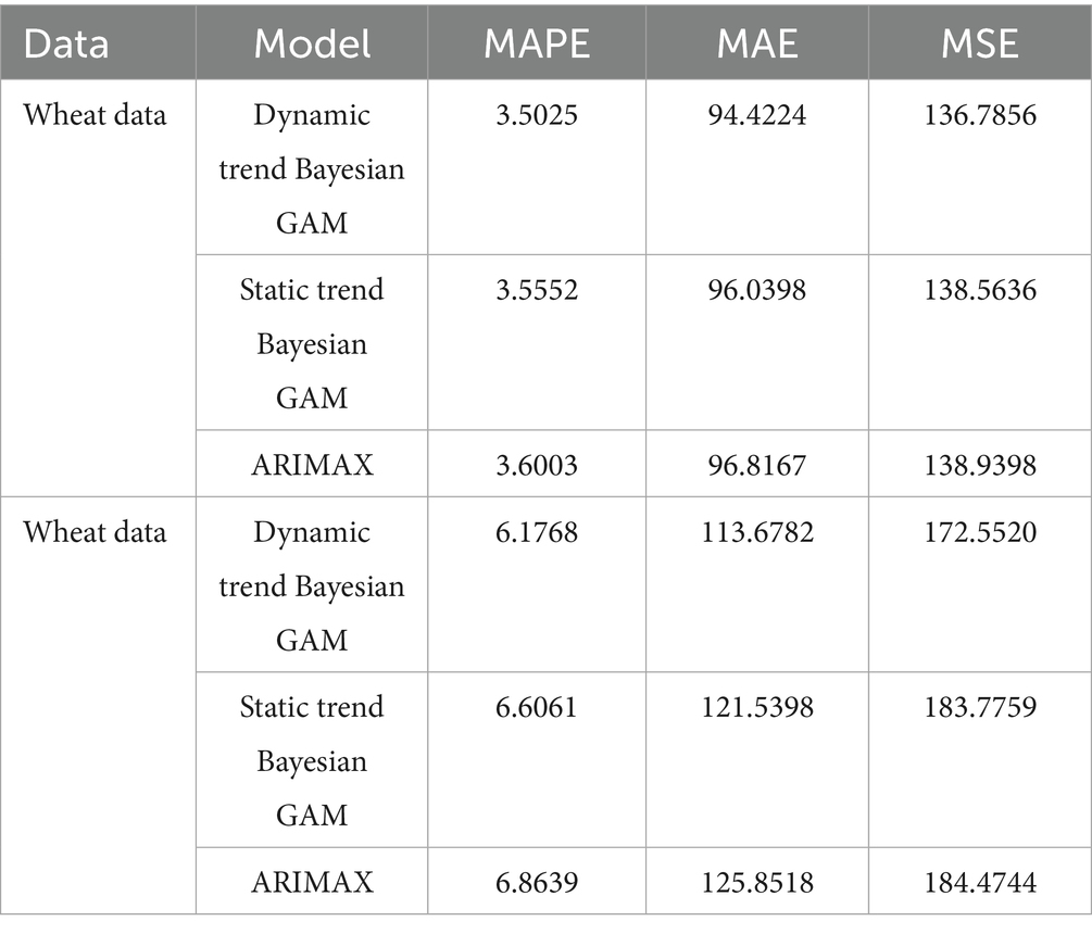
Table 6. Prediction (in-sample) evaluations.
Lower MAPE, MAE, and MSE indicate that a model performs well. In Table 4, we observe that the performance metrics for the trend or Bayesian models are smaller than those of the ARIMA models. This indicates that the Bayesian models outperform the ARIMA models for the in-samples estimates for both wheat and white maize prices. The lower MAPE, MAE, and MSE values for the dynamic local trend models in comparison to the static trend models also indicate superiority of the dynamic trend models over both the ARIMA and the static trend models.
The observed superiority confirms the efficiency of the trend model that was observed in Section 4.3. However, a better trained model may not necessarily yield accurate forecasts, thus the need to assess the performance of the model on unseen data. In this regard, we consider the LOO estimates. On the surface, a look at the LOO estimates indicates that static trend models are comparatively superior to dynamic trend models. This is because they have relatively higher expected logarithmic predictive density (elpd_loo) and lower leave-one-out information criterion(looic) values. However, the ratio of the elpd_loo differences(elpd_diff) to the standard error of elpd_loo (se_diff) is −0.275 for the maize data and −1.417 suggest that there are no significant differences between the two respective models. However, the estimated static trend model for the maize model is not reliable, since it has an observation whose Pareto k value is greater than 0.7 as indicated in Table 3. Furthermore, since LOO uses almost the entire data set for training, the model might capture noise instead of the underlying pattern, which may lead to overfitting; thus, the model may perform poorly on new and unseen data. It is therefore imperative to comprehensively assess the estimated models using a complete set of data that were not part of the model training phase.
In this regard, we assess the performance of the proposed model in comparison to the benchmarked models (static trend and ARIMA) for several forecasting horizons including short-term horizons (1, 3 and 7 months ahead) and long-term horizons (36 and 48 months ahead) using the MAPE, MAE and MSE loss functions as reported in Table 7. Evidence from the table suggests that the dynamic local trend and the static trend Bayesian models outperform the ARIMA models at all horizons except horizon 1. A comparison of the Bayesian models reveals that the dynamic local trend model is superior to the static trend model at all horizons except horizon 7. With reference to the maize data, the evidence seems to be pointing towards the general superiority of the static-trend Bayesian model in comparison to the dynamic local trend Bayesian model. However, since the LOO estimates for the static trend Bayesian model indicate a higher Pareto k value for the first observation, the observed superiority may be due to over-fitting, therefore we cannot make reliable conclusions or generalizations. Hence, we can only compare the performance of the dynamic local trend Bayesian and ARIMA models. On this note, the ARIMA performs better at horizon 1 and 3 than the dynamic trend Bayesian model while the dynamic local trend Bayesian model outperforms the ARIMA model at horizons 7, 36 and 48.
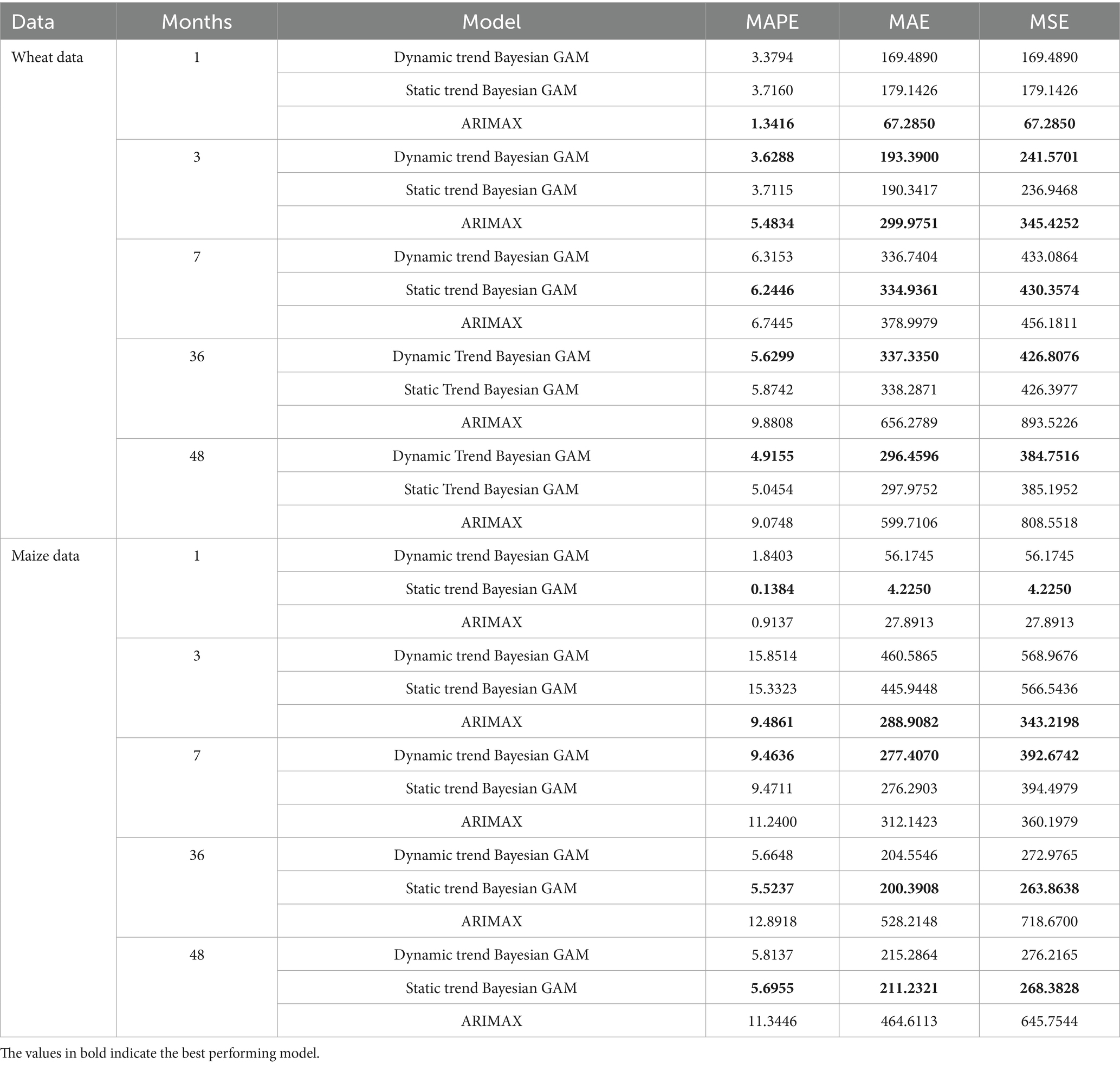
Table 7. Forecast (out-of-sample) comparison evaluations.
From the assessment of the LOO estimates and the loss function, it can be concluded that the Bayesian models generally perform better than the ARIMA models; however, the ARIMA models have potential of producing more accurate in the short term; especially up to three forecast horizons. Among the Bayesian models, the dynamic local trend model is generally superior to the static trend model because it produced more accurate long-term forecasts than the static model and may be competitive for short-term forecasting, as was the case of the wheat price data in this study. This conclusion suggests that the incorporation of dynamic local trends into the Bayesian GAM has the potential to improve model efficiency as well as prediction and forecast accuracy. It is therefore recommended that for short-term (except for one horizon ahead) and long-term forecasting of grain prices and other speculative asset prices, the dynamic local trend Bayesian GAM is recommended, while the ARIMA model is recommended for 1-day ahead forecasts.
4.5 Interpretations and discussion
To improve the forecast performance of the proposed Bayesian model while simultaneously understanding the complex dynamics among grain price external factors, past inflation (consumer price) and rainfall (precipitation indices) were incorporated into the model building process. Tables 4, 5 report the estimated parameters for the models, which include the smoothing spline hyperparameters, correlation structure, multilevel hyperparameters for the trend, regression estimates, and other distributional parameters. Other estimates such as the credible intervals (CI) are also reported.
From Tables 4, 5, it is observed that the smoothing spline hyperparameters parameters for all models are significant since zero cannot be found within the respective credible intervals, thus indicating that the Bayesian models were able to capture the nonlinear and complex relationships existing between the variables and the prices. The distributional parameters for all models are also significant, suggesting that the student-t distribution was able to capture the tail properties of the respective data. Furthermore, the autoregressive estimates were statistically significant, which indicates that the model was able to capture the underlying autocorrelation structures in the models. In the regression coefficients, the intercept parameters for all models are significant, which justifies the inclusion of the intercept term in the model.
A look at the local trend estimates also indicates a significant variability in the local trend intercept and slopes, which may be due to localized events across the years. The variability is more prominent in the local trend intercept (where it, respectively, averaged at R33.81 and R125.26 per year for wheat and maize prices) compared to the respective annual averages of R0.32 and 1.27 for the local trend slopes for wheat and maize prices. Maize prices have higher local trend variabilities compared to wheat prices as observed in the average estimated standard deviations, highlighting the volatile nature of maize prices compared to wheat prices as observed in Ceballos et al. (45). The results suggest significant heterogeneity in global trend across the years, while consistent but significant local time-specific variabilities also exist across the years. Observations from Figure 6 confirm the changing local trends over the years for the prices of maize and wheat. The greatest change in the magnitude of the local trends for maize and wheat prices occurred between 2002 and 2003. The decline in wheat prices coincides with the increase in wheat imports from more than 458,518 tonnes to more than a million tonnes from the 2003 and 2004 marketing year (46) which caused a decline in local market prices for reasons such as increased supply and market saturation. The decline in maize prices also coincided with the appreciation of the rand, which gained approximately 14%. Furthermore, there was a decrease in anticipated exports to neighbouring countries, which led to high stock levels totalling more than 2.5 million tons.
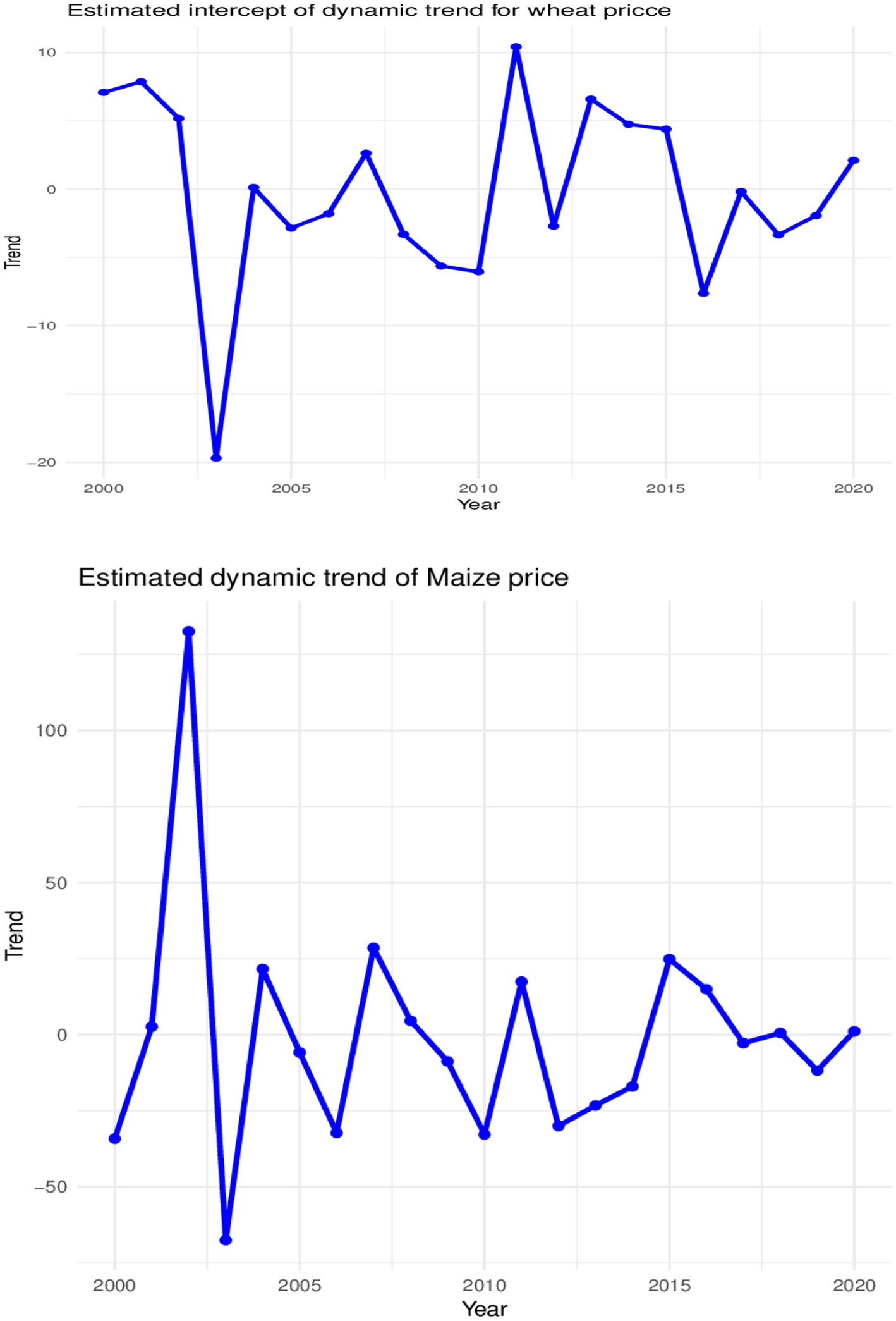
Figure 6. Estimated dynamics local trends for wheat and maize prices.
In terms of the impacts of inflation and rainfall on maize and wheat prices, Tables 4, 5 show that, while the average direction of the impact of previous inflation rates on maize and wheat prices is positive and significant (credible interval does not contain zero), the impacts of previous precipitation amount on prices are negative and significant (credible interval does not contain zero) for maize prices but not significant for wheat prices (credible interval contains zero). These results indicate that the previous increase in inflation generally leads to proportionally higher current maize and wheat prices, while a rise in the previous precipitation led to proportionally lower maize and wheat prices. However, a look at the conditional plots in Figures 7, 8 reveal that not all increases in inflation led to an increase in maize and wheat prices and not all increases in rainfall also led to a reduction in wheat and maize prices. For example, Figure 7 indicates that changes in inflation lead to sustained increases in maize prices until an index of 100 where maize prices steadily declined amid an increasing price index until the decline bottomed up at approximately an index of 110 before maize prices began to rise at a level with rising consumer price indices. Therefore, these complex relationships observed are nonlinear in nature; specifically, they are polynomial in nature. The observed relationship therefore implies that similar proportional increases in inflation do not always lead to similar proportional increase in maize and wheat prices, while similar proportional increases in precipitation do not always lead to similar proportional decreases in prices.
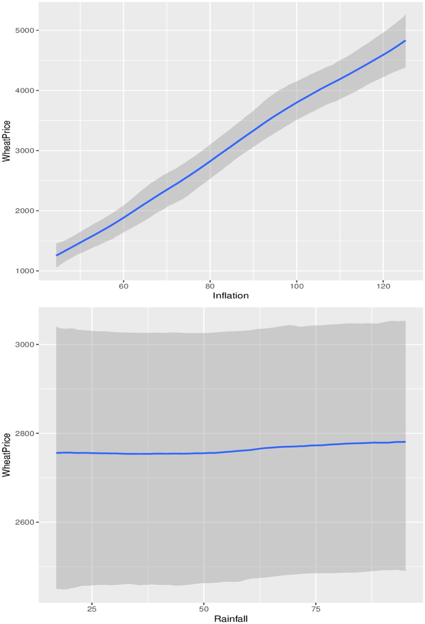
Figure 7. Conditional impact of inflation and rainfall on wheat prices.
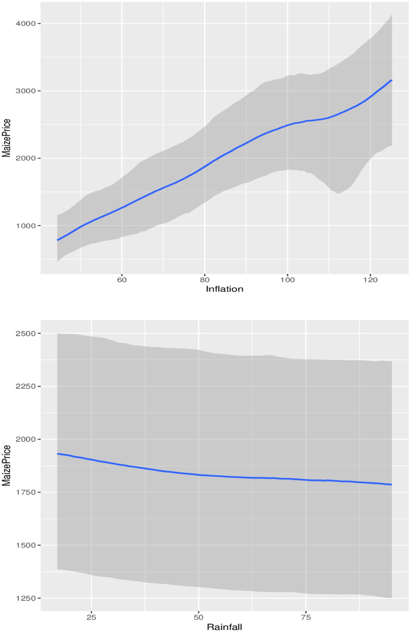
Figure 8. Conditional impact of inflation and rainfall on maize prices.
The observed non-linear dynamics of the grain price-inflation relationship may be due to factors such as previous exchange rate dynamics, market perception and sentiment, supply chain factors, government policies, and trade dynamics, among others (47–49). For example, previous government interventions, such as subsidies for maize and wheat or tariffs on imports, can affect the dynamics of futures grain price-inflation relationships (47, 49). This could lead to maize futures prices that do not reflect expected general or proportional inflation rates. Furthermore, global market conditions such as previous changes in global maize production, trade policies, and international demand can distort the grain price-inflation relationship (48); therefore, the surplus or deficit of wheat in other regions can influence futures prices regardless of the previous domestic inflation rate, which may lead to the observed polynomial grain price-inflation dynamics.
The observed non-linear impacts of precipitation on maize and wheat prices indicate a direct impact of rainfall on crop yields, crop quality, and agricultural productivity, which affect supply and demand, which in turn affect maize and wheat prices. Precipitation can affect crop yield positively or positively. Adequate and timely rainfall is crucial for optimal growth and development of maize and wheat; therefore, sufficient moisture can lead to high crop yields, which can improve supply and potentially lower prices. However, insufficient rainfall or reduced amounts of precipitation can reduce crop yields, leading to higher prices for both maize and wheat. For example, in Figure 8, consistent increases in precipitation indices were associated with lower maize prices until it slightly stabilized between 62.5 and 75% before continuing with the price decline. In the case of wheat, as observed in Figure 8, prices were slightly lower and stable for precipitation indices of up to 50% and then steadily increased between 50 and 75% before settling above 75%.
Although the non-linear impact observed by precipitation on wheat prices appears to be on the increase side compared to the price of maize, both impacts are negative. This can be supported by the average estimates in Tables 4, 5 which indicate an average reduction of R2.32 for maize compared to the reduction of R4.21 in the price of wheat for the same amount of change in rainfall. The relatively higher reduction in maize prices due to increased rainfall compared to wheat prices is supported by the tolerance mechanisms of both crops. Wheat is more tolerant to drought than maize and can grow successfully with relatively smaller amounts of rainfall per growing season, depending on the variety and environmental conditions (50). However, wheat has a relatively shallow root system, so excessive rainfall can result in root diseases, reduced oxygen availability, and ultimately decline in production due to waterlogging (51).
Other factors that may explain the impact of rainfall on prices include market price speculation and the hoarding of commodities by farmers and investors. Farmers and traders often adjust their expectations of future prices based on weather forecasts. Anticipation of adverse weather conditions, such as droughts or excessive rains, can lead to speculation that can increase prices even before actual crop losses are realized (52). In addition, when rainfall patterns are uncertain, investors and consumers can start to hoard grains, which can temporarily increase prices before harvests are confirmed.
5 Conclusion
This study aimed to forecast the future prices of maize and wheat in South Africa using flexible Bayesian dynamic local trend GAMs. The models were then compared to the static trend Bayesian GAM model (where the local trend is not modelled) and the ARIMA model. External factors such as inflation and rainfall that are known to affect grain prices were incorporated into the models to improve prediction and forecast accuracy. Subsequently, this also allowed us to understand the non-linear impact dynamics of these factors on wheat and maize prices. The data used include aggregated monthly prices of wheat and white maize futures, consumer prices, and precipitation indices. Based on the assessment of the estimated model and the examination of the impacts of consumer price and precipitation indices, the key findings of the study are summarized below.
In terms of parameter estimation efficiency, dynamic local trend models generally produced lower posterior standard deviation and shorter credible intervals, suggesting that added complexity and flexibility generally improved efficiency of parameter estimations because the models were able to accurately capture the underlying changing uncertainty around the local trends in the prices of maize and wheat. Subsequently this led to improved posterior predictions and forecasts, thus the models were generally superior to the static local trend models for long-term posterior forecasts. For wheat price-data, dynamic local trend models produced competitive short-term forecasts, except for forecasts a step ahead, where ARIMA models were superior. Hence, the dynamic local trend model has potential to improve short-term forecasts.
Evidence from the trend estimates suggests significant variability in the local trend intercept and slopes which may be due to localized events across the years. Local trend variabilities are more prominent in local intercepts than in local slopes for prices of both grains; however, maize prices have higher local trend variabilities compared to wheat prices as observed in the average estimated standard deviations, thus highlighting the volatile nature of maize prices compared to wheat prices. The evidence also revealed prominent shifts in the magnitude of the local trends in wheat and maize prices occurred between 2002 and 2003. These shifts could be attributed to factors such as increased supply and market saturation, the appreciation of the rand, and the anticipated decline in exports to neighboring countries.
From the estimated impacts, a direct significant nonlinear polynomial impact of inflation on wheat and maize prices was observed, suggesting that similar proportional increases in inflation do not always lead to similar proportional increases in maize and wheat prices, while similar proportional increases in precipitation do not always lead to similar proportional decreases in prices. Non-linear factors such as previous exchange rate dynamics, market perception and sentiment, supply chain factors, government policies, and trade dynamics were identified as some of the possible causes of the non-linear relationships between inflation and grain prices. It was also observed that although the impacts of rainfall on wheat and maize prices were indirect and non-linear, only the impact on maize prices as significant, so changes in the amount of rainfall may not proportionately lead to lower levels of grain prices. Factors such as crop yields, quality of crops, agricultural productivity which are directly affected by rainfall and consequently affect supply and demand were identified as possible causes of the observed non-linear relationships. Furthermore, speculation on market prices and the hoarding of commodities by farmers and investors due to anticipated adverse weather conditions, such as droughts or excessive rain, were also identified as a possible cause.
The contributions of this study are three-fold: (1) the identification of a better alternative framework in forecasting grain prices, (2) the need to model local trends, and (3) the unveiling of the complex dynamics of the relationships among grain prices and the exogenous factors-consumer price and precipitation indices. These contributions are summarized below.
• The study has made contributions to literature by unveiling the superiority of the Bayesian GAM of dynamic local trend over the static version and the commonly used ARIMA model, thus providing a better alternative model in forecasting grain prices and the impacts of external pressures on grain prices.
• Furthermore, we argue that heterogeneity exists in single subject nonstationary time series data due to data aggregation effects, although this can obscure heterogeneity in local trend fluctuations when ignored, thus potentially yielding biased fixed effect estimates and less accurate predictions and forecasts when ignored. This argument has been empirically substantiated in this study, thus providing support for the incorporation of dynamic local trends in single subject nonstationary time in models where this property is not explicitly modelled.
• Previous studies have mainly focused on the impacts of food prices on inflation (53–55), but the reverse relationship has been grossly neglected, although inflation can induce grain prices through a feedback mechanism due to factors such as cost of inputs, purchasing power and substitution effect, among others. Therefore, this study has contributed to our understanding of the inflation-grain price feedback mechanisms. Particularly the non-linear feedback mechanisms which have also grossly been neglected even in the most studied inflation-grain price feedback mechanisms.
• Furthermore, the study has made contributions to understanding the complex dynamics of the impact of precipitation, which is a major driver of grain production. In particular, the contribution is in the direction of revealing the nonlinear impacts of precipitation on the futures prices of wheat and maize, which previous studies such as Aker (56) have not considered.
• Finally, most studies have not examined the nonlinear lagged effect of inflation and precipitation on maize and wheat prices, especially within the South African context; therefore, our study is also a contribution in this regard.
In conclusion, the dynamic Bayesian GAM framework is identified as a better alternative to the ARIMA model when forecasting and modelling grain prices. However, the dynamic local trend version is preferred to the static trend version due to its efficiency and superiority in forecasting single subject non-stationarity times series such as maize and wheat prices. Therefore, the proposed dynamic local trend Bayesian GAM is recommended for forecasting grain prices and examining the complex relationships in single subject nonstationary time series and exogenous factors.
A major limitation of our proposed model and dynamic Bayesian GAM in general is their reliance on heavy computational power and memory, especially with large datasets which may prolong estimation time or fail to run in the absence of adequate computational power and memory. To alleviate this problem, we recommend the use of computers with high performance and memory capabilities. It is also recommended that parallel computation capabilities of different programming languages such as R and within the MCMC algorithm itself be used to reduce computational time.
Data availability statement
Publicly available datasets were analyzed in this study. The datasets were extracted and compiled from different sources including www.sagis.org.za/safex_historic.html, www.investing.com and https://giovanni.gsfc.nasa.gov/giovanni/. The compiled list is available upon request.
Author contributions
AA: Conceptualization, Formal analysis, Funding acquisition, Methodology, Resources, Software, Supervision, Writing – original draft. EK: Data curation, Formal analysis, Funding acquisition, Investigation, Writing – review & editing. LC: Conceptualization, Funding acquisition, Writing – original draft, Writing – review & editing. MA: Funding acquisition, Validation, Writing – review & editing.
Funding
The author(s) declare that financial support was received for the research and/or publication of this article. This study was founded by the Centre for Global Change at Sol Plaatje University, Kimberley, South Africa under the project titled “The changing planet and its impact on food security in sub-Saharan Africa”.
Acknowledgments
The authors thank the Centre for Global Change at Sol Plaatje, which provided funding for this study. We also extend our gratitude to our various institutions that provided us with all the necessary support during the course of this study.
Conflict of interest
The authors declare that the research was conducted in the absence of any commercial or financial relationships that could be construed as a potential conflict of interest.
Generative AI statement
The authors declare that Gen AI was used in the creation of this manuscript. Generative AI was used to search for ideas. Supporting articles for those ideas were then accessed and thoroughly reviewed after which the idea was refined and used in the manuscript. Such cases represent about 10% of the total content of the article.
Publisher’s note
All claims expressed in this article are solely those of the authors and do not necessarily represent those of their affiliated organizations, or those of the publisher, the editors and the reviewers. Any product that may be evaluated in this article, or claim that may be made by its manufacturer, is not guaranteed or endorsed by the publisher.
Footnotes
1. ^An NP-hard problem involves computational problems where known algorithm cannot efficiently solve all instances (i.e., in polynomial time).
2. ^The first value within the brackets indicates the autoregressive (AR) term, the second specifies the order of integration, and the last value represents the moving average (MA) term.
References
1. Wudil, AH, Usman, M, Rosak-Szyrocka, J, Pila, L, and Boye, M. Reversing years for global food security: a review of the food security situation in sub-Saharan Africa (SSA). Int J Environ Res Public Health. (2022) 19:14836. doi: 10.3390/ijerph192214836
2. World Bank. Putting Africans at the heart of food security and climate resilience (2022). Available online at: https://www.worldbank.org/en/news/immersive-story/2022/10/17/putting-africans-at-the-heart-of-food-security-and-climate-resilience (Accessed February 7, 2025)
3. Dlamini, SN, Craig, A, Mtintsilana, A, Mapanga, W, Du Toit, J, Ware, LJ, et al. Food insecurity and coping strategies and their association with anxiety and depression: a nationally representative south African survey. Public Health Nutr. (2023) 26:705–15. doi: 10.1017/S1368980023000186
4. Sun, F, Meng, X, Zhang, Y, Wang, Y, Jiang, H, and Liu, P. Agricultural product price forecasting methods: a review. Agriculture. (2023) 13:1671. doi: 10.3390/agriculture13091671
6. Brignoli, PL, Varacca, A, Gardebroek, C, and Sckokai, P. Machine learning to predict grains futures prices. Agric Econ. (2024) 55:479–97. doi: 10.1111/agec.12828
7. Wang, Z, French, N, James, T, Schillaci, C, Chan, F, Feng, M, et al. Climate and environmental data contribute to the prediction of grain commodity prices using deep learning. J Sustain Agric Environ. (2023) 2:251–65. doi: 10.1002/sae2.12041
8. Diop, MD, and Kamdem, JS. Multiscale agricultural commodities forecasting using wavelet-SARIMA process. J Quant Econ. (2023) 21:1–40. doi: 10.1007/s40953-022-00329-4
9. Albuquerquemello, VPD, Medeiros, RKD, Jesus, DPD, and Oliveira, FAD. The role of transition regime models for corn prices forecasting. Rev Econ Sociol Rural. (2022) 60:e236922. doi: 10.1590/1806-9479.2021.236922
10. Saxena, K, and Mhohelo, DR. Modelling of maize prices using autoregressive integrated moving average (ARIMA). Int J Stat Appl Math. (2020) 5:229–45.
11. Lai, Y, and Dzombak, DA. Use of the autoregressive integrated moving average (ARIMA) model to forecast near-term regional temperature and precipitation (2020). Available online at: https://journals.ametsoc.org/view/journals/wefo/35/3/waf-d-19-0158.1.xml (Accessed February 7, 2025)
12. Jadhav, V, Reddy, BVC, and Gaddi, GM. Application of ARIMA model for forecasting agricultural prices. J Agr Sci Tech. (2017) 19:981–92.
13. Jin, B, and Xu, X. Wholesale price forecasts of green grams using the neural network. Asian J Econ Bank. (2024). doi: 10.1108/ajeb-01-2024-0007
14. Crockett, MJ, Bai, X, Kapoor, S, Messeri, L, and Narayanan, A. The limitations of machine learning models for predicting scientific replicability. Proc Natl Acad Sci. (2023) 120:e2307596120. doi: 10.1073/pnas.2307596120
15. Barbierato, E, and Gatti, A. The challenges of machine learning: a critical review. Electronics. (2024) 13:416. doi: 10.3390/electronics13020416
16. Ghorbani, A, Kim, MP, and Zou, J. A distributional framework for data valuation (2020). Available online at: https://arxiv.org/abs/2002.12334v1 (Accessed May 15, 2025)
17. Lagemann, K, Lagemann, C, Taschler, B, and Mukherjee, S. Deep learning of causal structures in high dimensions under data limitations. Nat Mach Intell. (2023) 5:1306–16. doi: 10.1038/s42256-023-00744-z
18. Pawelczyk, M, Datta, T, van-den-Heuvel, J, Kasneci, G, and Lakkaraju, H. Probabilistically robust recourse: navigating the trade-offs between costs and robustness in algorithmic recourse (2022). Available online at: https://arxiv.org/abs/2203.06768v4 (Accessed May 15, 2025)
19. Rawal, K, Kamar, E, and Lakkaraju, H. Algorithmic recourse in the wild: understanding the impact of data and model shifts (2020). Available online at: https://arxiv.org/abs/2012.11788v3 (Accessed May 15, 2025)
20. Artelt, A, and Hammer, B. On the computation of counterfactual explanations—a survey (2019). Available online at: http://arxiv.org/abs/1911.07749 (Accessed May 15, 2025)
21. Verma, R. Hedging model using R |how investors really save money in market!!. Medium (2023). Available online at: https://medium.com/@ravikant.verma6991/hedging-model-using-r-how-investors-really-save-money-in-market-807184ebe620 (Accessed February 18, 2024)
22. Follett, L, and Vander Naald, B. Explaining variability in tourist preferences: a Bayesian model well suited to small samples. Tour Manag. (2020) 78:104067. doi: 10.1016/j.tourman.2019.104067
23. Wellington, MJ, Lawes, R, and Kuhnert, P. A framework for modelling spatio-temporal trends in crop production using generalised additive models. Comput Electron Agric. (2023) 212:108111. doi: 10.1016/j.compag.2023.108111
24. Ravindra, K, Rattan, P, Mor, S, and Aggarwal, AN. Generalized additive models: building evidence of air pollution, climate change and human health. Environ Int. (2019) 132:104987. doi: 10.1016/j.envint.2019.104987
25. Yang, L, Ren, R, Gu, X, and Sun, L. Interactive generalized additive model and its applications in electric load forecasting (2023). Available online at: http://arxiv.org/abs/2310.15662 (Accessed May 12, 2025)
26. Chen, K, O’Leary, RA, and Evans, FH. A simple and parsimonious generalised additive model for predicting wheat yield in a decision support tool. Agric Syst. (2019) 173:140–50. doi: 10.1016/j.agsy.2019.02.009
27. Yee, TW. The VGAM package for categorical data analysis. J Stat Soft. (2010) 32:1–34. doi: 10.18637/jss.v032.i10
28. Clark, NJ, and Wells, K. Dynamic generalised additive models (DGAMs) for forecasting discrete ecological time series. Methods Ecol Evol. (2023) 14:771–84. doi: 10.1111/2041-210X.13974
29. Rajaguru, G, Lim, S, and O’Neill, M. A review of temporal aggregation and systematic sampling on time-series analysis. J Account Lit. (2025) 47:110–28. doi: 10.1108/JAL-09-2024-0237
30. Zhou, L. Application of ARIMA model on prediction of China’s corn market. J Phys Conf Ser. (2021) 1941:012064. doi: 10.1088/1742-6596/1941/1/012064
31. Räz, T. ML interpretability: simple isn’t easy. Stud Hist Phil Sci. (2024) 103:159–67. doi: 10.1016/j.shpsa.2023.12.007
32. Hastie, T, and Tibshirani, R. Generalized additive models. Stat Sci. (1986) 1:297–310. doi: 10.1214/ss/1177013604
33. Nelder, JA, and Wedderburn, RWM. Generalized linear models. J R Stat Soc Ser A Stat Soc. (1972) 135:370. doi: 10.2307/2344614
34. Wood, SN. Fast stable restricted maximum likelihood and marginal likelihood estimation of semiparametric generalized linear models. J R Stat Soc Ser B Stat Methodol. (2011) 73:3–36. doi: 10.1111/j.1467-9868.2010.00749.x
35. Lin, X, and Zhang, D. Inference in generalized additive mixed models by using smoothing splines. J R Stat Soc Ser B Stat Methodol. (1999) 61:381–400. doi: 10.1111/1467-9868.00183
36. Solonen, A, and Staboulis, S. On Bayesian generalized additive models (2023). Available online at: http://arxiv.org/abs/2303.02626 (Accessed May 12, 2025)
37. Perperoglou, A, Sauerbrei, W, Abrahamowicz, M, and Schmid, M. A review of spline function procedures in R. BMC Med Res Methodol. (2019) 19:46. doi: 10.1186/s12874-019-0666-3
38. Spade, DA. Markov chain Monte Carlo methods: theory and practice. In: Handbook of statistics Elsevier; (2020); p. 1–66. Available online at: https://linkinghub.elsevier.com/retrieve/pii/S0169716119300379 (Accessed February 13, 2025).
39. Chib, S. Markov chain Monte Carlo methods: computation and inference. In: Handbook of econometrics. Elsevier; (2001); p. 3569–3649. Available online at: https://linkinghub.elsevier.com/retrieve/pii/S1573441201050103 (Accessed February 13, 2025)
40. Betancourt, M. A conceptual introduction to Hamiltonian Monte Carlo (2017). Available online at: https://arxiv.org/abs/1701.02434 (Accessed February 13, 2025)
41. Juárez, MA, and Steel, MFJ. Model-based clustering of non-Gaussian panel data based on skew-t distributions. J Bus Econ Stat. (2010) 28:52–66. doi: 10.1198/jbes.2009.07145
42. Lewandowski, D, Kurowicka, D, and Joe, H. Generating random correlation matrices based on vines and extended onion method. J Multivar Anal. (2009) 100:1989–2001. doi: 10.1016/j.jmva.2009.04.008
43. Bürkner, PC. brms: an R package for Bayesian multilevel models using Stan. J Stat Soft (2017);80. Available online at: http://www.jstatsoft.org/v80/i01/ (Accessed February 12, 2025)
44. Kruschke, JK, Front matter. In: Doing Bayesian data analysis (2nd) Boston: Academic Press; (2015); p. i–ii. Available online at: https://www.sciencedirect.com/science/article/pii/B9780124058880099992 (Accessed 2025 Feb 12)
45. Ceballos, F, Hernandez, MA, Minot, N, and Robles, M. Transmission of food price volatility from international to domestic markets: evidence from Africa, Latin America, and South Asia. In: Food price volatility and its implications for food security and policy. Springer, Cham; (2016). p. 303–328. Available online at: https://link.springer.com/chapter/10.1007/978-3-319-28201-5_13 (Accessed May 22, 2025)
46. Sihlobo, W. Wheat in South Africa (2022). Available online at: https://wandilesihlobo.com/2022/03/22/wheat-in-south-africa/ (Accessed May 21, 2025)
47. Chapoto, A, and Jayne, TS. The impacts of trade barriers and market interventions on maize price predictability: evidence from Eastern and Southern Africa (2009). Available online at: https://ageconsearch.umn.edu/record/56798 (Accessed February 12, 2025)
48. De Wet, F, and Liebenberg, I. Food security, wheat production and policy in South Africa: reflections on food sustainability and challenges for a market economy. J Transdiscipl Res (2018) 14:a407. doi: 10.4102/td.v14i1.407
49. McDonald, S, Punt, C, Rantho, L, and Van Schoor, M. Costs and benefits of higher tariffs on wheat imports to South Africa. Agrekon. (2008) 47:19–51. doi: 10.1080/03031853.2008.9523789
50. Nezhadahmadi, A, Prodhan, ZH, and Faruq, G. Drought tolerance in wheat. Sci World J. (2013) 1:610721. doi: 10.1155/2013/610721
51. Timsina, J, and Connor, DJ. Productivity and management of rice–wheat cropping systems: issues and challenges. Field Crop Res. (2001) 69:93–132. doi: 10.1016/S0378-4290(00)00143-X
52. Letta, M, Montalbano, P, and Pierre, G. Weather shocks, traders’ expectations, and food prices. Am J Agric Econ. (2022) 104:1100–19. doi: 10.1111/ajae.12258
53. Ahsan, N, Amin, A, Hassan, J, and Mahmood, T. Effects of inflation on agricultural commodities. IJASD. (2020) 2:105–11.
55. Tule, MK, Salisu, AA, and Chiemeke, CC. Can agricultural commodity prices predict Nigeria’s inflation? J Commod Mark. (2019) 16:100087. doi: 10.1016/j.jcomm.2019.02.002
56. Aker, JC. Rainfall shocks, markets, and food crises: evidence from the Sahel. SSRN J. (2008). Available online at: http://www.ssrn.com/abstract=1321846 (Accessed February 12, 2025)
Keywords: local trend, Bayesian GAMS, grain prices, nonlinearity, non-stationarity
Citation: Antwi A, Kammies ET, Chaka L and Arasomwan MA (2025) Forecasting South African grain prices and assessing the non-linear impact of inflation and rainfall using a dynamic Bayesian generalized additive model. Front. Appl. Math. Stat. 11:1582609. doi: 10.3389/fams.2025.1582609
Edited by:
George Michailidis, University of Florida, United StatesReviewed by:
Jiangjiang Zhang, Hohai University, ChinaArindam Fadikar, Argonne National Laboratory (DOE), United States
Copyright © 2025 Antwi, Kammies, Chaka and Arasomwan. This is an open-access article distributed under the terms of the Creative Commons Attribution License (CC BY). The use, distribution or reproduction in other forums is permitted, provided the original author(s) and the copyright owner(s) are credited and that the original publication in this journal is cited, in accordance with accepted academic practice. No use, distribution or reproduction is permitted which does not comply with these terms.
*Correspondence: Albert Antwi, YWxiZXJ0LmFhbnR3aUBvdXRsb29rLmNvbQ==
†ORCID: Albert Antwi, orcid.org/0000-0002-3571-4850