On transaction costs in minimum-risk portfolios: insights into risk parity and asset allocation

In minimal risk portfolios, costs associated with transactions are essential in calculating the net performance. The transaction costs of maintaining such portfolios are predominantly negative due to the fact that traditional portfolio optimization strategies, which focus solely on risk and return, neglecting transaction costs typically incurred through rebalancing. This research analyzes the impact of costs associated with transactions while constructing minimum risk portfolios centered around risk parity models and provides a way to control those costs. We investigate the performance of portfolios under fixed and flexible costs and include these parameters in the optimization model to achieve more realistic results. Applying real-world data on conventional stock portfolios and highly volatile cryptocurrency markets, we demonstrate the performance of mean–variance optimization (M-V), risk parity with standard deviation (RP-Std), and risk parity with Conditional Value at Risk (RP-CVaR) through empirical data for both stock portfolios and cryptocurrencies. We found that potential transaction costs can cause portfolio returns to change by anywhere between 0.5 to 2% per year depending on how often one trades, and market conditions. By highlighting how crucial it is to incorporate transaction costs into the decision-making process, this study contributes to the expanding literature of research on portfolio optimization. For investors looking to create and manage their portfolios in a way that balances risk, return, and cost effectiveness, our findings offer useful insights. Future studies might investigate adaptive models that dynamically adapt to shifting cost structures and market situations, or they could generalize these findings to other asset classes.

1 Introduction

Minimum risk portfolios seek to minimize risk while achieving a certain threshold of returns. As such, these portfolios are constructed using mean–variance optimization or other risk-minimizing techniques. Yet, in practice, the construction and management of such portfolios have hidden costs such as brokerage commissions, bid-ask spreads, taxes, and market impact costs. These transaction costs can offset the benefits from portfolio optimization, in particular from active strategies that require constant rebalancing. This research examines the impact of transaction costs on minimum risk portfolios, in addition to existing literature on how to model these costs in a portfolio optimization framework.

Transaction costs are a significant addition to the problem, which is both difficult from a control perspective because the solution now requires singular control and extremely relevant from a financial one. Some works propose a data-driven approach to portfolio optimization that tackles transaction costs and estimation error simultaneously by treating the transaction costs as a regularization term to be calibrated (1).

In the financial markets, liquidity is crucial and influences a wide range of variables, such as risk, returns, and stock prices. The order book, which records traders’ orders to purchase and sell stocks at various price points, is typically used to gauge liquidity in the stock market (2).

Few portfolio managers in the real world ignore transaction costs at the portfolio-selection stage and simply pay them after the fact. Doing so can be expected to result in worse net performance (that is, performance after transaction costs), at least for high-turnover strategies. Therefore, Ledoit and Wolf propose a way to account for transaction costs at the portfolio-selection stage (3).

Transaction costs are a source of concern for portfolio managers. Due to the change in expectation of a future return of securities, most applications of portfolio optimization involve the revision of an existing portfolio. This revision entails both purchases and sales of securities along with transaction costs (4).

By considering investor’s preferences such as transaction costs and liquidity needs, Wang et al. have developed a class of uncertain mean-CVaR portfolio models that are more realistic to real-world stock trading markets (5).

In their paper, Gou et al. include the peer effect into the return forecast where the predicted return of one risky asset not only depends on its past return data but also the other risky assets in the financial market, which gives a more accurate prediction (6). An adaptive moving average method with peer impact (AOLPI) is proposed, in which the decaying factors can be adjusted automatically in the investment process (6).

De Miguel et al. evaluate the out-of-sample performance of the sample-based mean–variance model, and its extensions designed to reduce estimation error, relative to the naive 1/N portfolio (7). Of the 14 models they evaluate across seven empirical datasets, none is consistently better than the 1/N rule in terms of Sharpe ratio, certainty-equivalent return, or turnover, which indicates that, out of sample, the gain from optimal diversification is more than offset by estimation error (7).

Transaction costs are the expenses incurred when buying or selling financial assets. They can be categorized into explicit costs (e.g., brokerage fees, taxes) and implicit costs (e.g., bid-ask spreads, market impact). In the context of minimum risk portfolios, transaction costs arise during initial portfolio construction, periodic rebalancing to maintain the desired risk profile and adjustments due to changes in market conditions or investor preferences

Studies have shown that transaction costs can reduce portfolio returns by 0.5 to 2% annually, depending on the trading frequency and market conditions (8).

Transaction costs can alter the risk–return profile of a portfolio. For instance, a portfolio optimized without considering transaction costs may appear efficient in theory but could underperform in practice due to the drag of these costs. Key impacts include:

• Reduced Net Returns: transaction costs directly reduce the net returns of a portfolio, making it harder to achieve the desired risk-adjusted performance (9).

• Suboptimal Asset Allocation: ignoring transaction costs may lead to the selection of assets that are expensive to trade, resulting in a suboptimal portfolio (10).

• Increased Tracking Error: for portfolios benchmarked against an index, transaction costs can increase tracking error, as frequent rebalancing may deviate from the benchmark (7).

As mentioned (4, 5, 7), most of the literature uses few models to optimize the financial portfolio with transaction cost due to their complexity to integrate and implement. Our focus is not only in the simple models like the uniform portfolio, or the traditional Mean Variance and Conditional Value at Risk, but also in the novelty of the Risk Parity models in the recent years. Integrating the transaction cost, with the traditional portfolio composed by stocks or the recent portfolios created using cryptocurrency (11), will make a better estimation for the investors and speculators in purpose to gain more from market.

The aim of this work is to present the comparison cases of transaction cost in case of fixed cost and variable cost between the minimum risk case and the Risk Parity cases. For the minimum risk we use the standard deviation and the Conditional Value at Risk as risk measures. The Risk Parity cases are calculated with three different methods, in which one uses the standard deviation and the other two the Conditional Value at Risk and the worst-case scenario that we call Risk Parity with CVaR Naïve.

This article is organized as follows: Section 2 outlines the theoretical framework for the models used. Section 3 considers case studies, and Section 4 concludes.

2 Models and methodology

The models used in this paper includes a variety of models with differing complexities, starting from the simplest Naïve or Uniform, passing through the traditional Mean Variance, Conditional Value at Risk, to the more recent Risk parity Strategies. From the optimization point of view, we also compare quadratic optimization (Mean Variance) with linear optimization (CVaR and Risk parity strategies).

Firstly, we describe a portfolio created by n-assets with allocation weights w = (w₁, w₂, …,w_n), the square root of the variance is given by

$\begin{array}{ll}{\sigma }_P\left(w\right)=\sqrt{\sum _{i=1}^n\sum _{j=1}^n{\sigma }_{\mathit{ij}}{w}_i{w}_j}=\sqrt{w\prime \mathit{\Lambda w}}& (1)\end{array}$

in which $\Lambda$ is the covariance matrix from for the returns.

If the returns are μ = (μ ₁, μ ₂, …, μ _n) then the constrain for the portfolio return is

$\begin{array}{ll}{\mu }_P=\sum _{i=1}^{n}w{\mu }_i=\mu \prime w& (2)\end{array}$

These two equations, Equations 1 and 2 are needed for the Mean Variance portfolio, in case that the short selling are not allowed (Equation 9), and the weights expressed in percentage of the investment (Equation 8).

The other model used in this paper is Expected Shortfall or (Equation 3) Conditional Value at Risk which can be calculated as follow:

$\begin{array}{ll}{\mathrm{ES}}_{\beta }\left(\mathrm{w}\right)=-\mathrm{E}[{\mu }_{\mathrm{P}}\mid {\mu }_P\le -{\mathrm{VaR}}_{\beta }(\mathrm{w}\left)\right]& (3)\end{array}$

As in continuous case (Equation 4), we have

$\begin{array}{ll}{\mathit{ES}}_{\beta }\left(w\right)=\frac{1}{\beta }{\int }_0^{\beta }{\mathrm{VaR}}_v\left(\mathrm{w}\right)\mathrm{d}v& (4)\end{array}$

With an $\beta \in (0,1)$

Also, with the Conditional Value at Risk, like in the case of Mean Variance, the short selling is not allowed ( $w\ge 0$ ), and the weights expressed in percentage of the investment. These two categories try to minimize the risk for a level of return, and if the constrain of expected returns is not considered (Equation 2), they will give the minimal risk of the portfolio. Usually, the models that rely on the expected return constrain tend to have high concentrations. For that the novice Risk Parity strategies are created.

The Equally Risk Contribution (risk parity condition) using the standard deviation as a risk measure (Equation 5) can be divided in totally risk contribution (Equation 6) of each asset i:

$\begin{array}{ll}{\mathit{TRC}}_i\left(w\right)=w_i\frac{\partial {\sigma }_P\left(w\right)}{\partial w_i}=y_i\frac{\partial {\sigma }_i^2+\sum _{j=1}^n{w}_i{\sigma }_{\mathit{ij}}}{{\sigma }_P\left(w\right)}=w_i\frac{{\left(\mathit{\Lambda w}\right)}_i}{\sqrt{w\prime \mathit{\Lambda w}}}& (5)\end{array}$

$\begin{array}{ll}\sum _{i=1}^m{\mathit{TRC}}_i\left(w\right)=\sum _{i=1}^n{w}_i\frac{{\left(\mathit{\Lambda w}\right)}_i}{\sqrt{w\prime \mathit{\Omega w}}}=\sqrt{w\prime \mathit{\Lambda w}}={\sigma }_P\left(w\right)& (6)\end{array}$

The Risk Parity model can be formulated as the following optimization problem (Equation 7):

$\begin{array}{ll}{w}^{\ast }=\text{argmin}\sum _{i=1}^n\sum _{j=1}^n{\left({\mathit{TRC}}_i\right(w)-{\mathit{TRC}}_j(w\left)\right)}^2& (7)\end{array}$

$\begin{array}{ll}\sum _{i=1}^n{w}_i=1& (8)\end{array}$

$\begin{array}{ll}{w}_i\ge 0& (9)\end{array}$

The same result starting from the Expected Shortfall given in Equations 3 and 4, which is equivalent to the ${\mathit{\text{CVaR}}}_{\alpha }\left(x\right)$ , as Tasche and Acerbi (12) and Stefanovits (13) showed in their work, under the condition that $E\left[X^{-}\right]<\infty$ . They used only in the case where the variables are normally distributed, which is far from the reality.

In the same way, we divide the Total Risk contribution for each asset i of a portfolio is given by the following expression (Equation 10):

$\begin{array}{ll}\mathit{TR}{C}_i^{{\mathit{ES}}_{\beta }\left(w\right)}\left(w\right)=w_i\frac{\partial {\mathit{ES}}_{\beta }\left(w\right)}{\partial w_i}& (10)\end{array}$

$\begin{array}{ll}\mathit{TR}{C}_i^{{\mathit{ES}}_{\beta }\left(w\right)}\left(w\right)=-w_{i}E[{\mu }_i\mid W\le -{\mathit{ES}}_{\beta }(w\left)\right]& (11)\end{array}$

$\begin{array}{ll}{\mathit{ES}}_{\beta }\left(w\right)=\sum _{i=1}^n\mathit{TR}{C}_i^{E{S}_{\beta }\left(w\right)}\left(w\right)=-\sum _{i=1}^n{w}_{i}E[{\mu }_i\mid W\le -{\mathit{VaR}}_{\beta }(w\left)\right]& (12)\end{array}$

Equations 11 and 12 are necessary for the numerical approximation in case of discrete data that we will use. Passing from standard deviation to Conditional Value at risk, we can study if there is a significant difference also in terms of transaction costs. The Risk parity strategies are considered as true diversification since they equalize the Total Risk contribution. From this point of view Mean Variance equalize the Marginal risk contribution given only by the part of the partial derivative. We also implement the worst-case scenario for the Conditional Value at risk. We call it Risk Parity with CVaR naïve.

After we calculate the optimal weights, we use them to calculate the transaction costs (Equation 13). If we will take in consideration the variable transaction cost:

$\begin{array}{ll}V{C}_i^t=\alpha {\sum }_{i=1}^n\mid w_i^{t+1}-w_i^t\mid & (13)\end{array}$

Where $w_i^t$ denotes the weight of asset i at time t and $\alpha$ is the variable cost.

For the fixed cost for the asset

$F{C}_i^t={\gamma }_i{\mathbb{I}}_{w_i^{t+1}\ne w_i^t}$

where:

${\mathbb{I}}_{w_i^{t+1}\ne w_i^t\text{ (14)}}=\{\begin{array}{c}1\mathit{\text{if}}{w}_i^{t+1}\ne w_i^t\\ 0\mathit{\text{if}}{w}_i^{t+1}=w_i^t\end{array}$

In Equation 14, ${\gamma }_i$ is the fixed cost applied.

In this index function in application, we put a threshold $\epsilon$ of tolerance for which if the difference is smaller than a certain limit (Equation 15), we consider them as equal

$\{\begin{array}{c}{w}_i^{t+1}\ne w_i^t\mathit{\text{if}}\mid w_i^{t+1}-w_i^t\mid >\epsilon \\ w_i^{t+1}=w_i^t\mathit{\text{if}}\mid w_i^{t+1}-w_i^t\mid <\epsilon \end{array}\text{ (15)}$

For the level of tolerance, we will have different results. The total cost at the time t is calculated as follows (Equation 16):

$\begin{array}{ll}{C}^t={\sum }_{i=1}^n(F{C}_i^t+V{C}_i^t)& (16)\end{array}$

Gârleanu and Pedersen provide empirical evidence that incorporating transaction costs into dynamic trading strategies improves net returns (14). In this case, we can include the transaction costs at the objective function (Equation 17):

$\begin{array}{c}max\\ w^t\end{array}{\sum }_{t=1}^T(w^t{\mathrm{\mu }}^t-C^t)\text{ (17)}$

We propose in case of minimum risk the following addition (Equation 18)

$\begin{array}{ll}min(\frac{1}{2}w\prime \mathit{\Lambda w}+C^t)& (18)\end{array}$

Since the framework is for the minimum risk, we can reach that by not including the expected portfolio return constrain. In case of minimum Conditional Value at Risk we change the risk measure in the objective function.

For the Risk Parity model the linear programing formulation including the transaction costs will be as follow (Equation 19):

$\begin{array}{ll}{w}^{\ast }=\text{argmin}(\sum _{i=1}^n\sum _{j=1}^n{\left({\mathit{TRC}}_i\right(w)-{\mathit{TRC}}_j(w\left)\right)}^2+C^t)& (19)\end{array}$

$\begin{array}{ll}\sum _{i=1}^n{w}_i=1& (20)\end{array}$

$\begin{array}{ll}{w}_i\ge 0& (21)\end{array}$

We do not allow the short selling (Equation 20) and express the budget invested in percentage of the total capital (Equation 21). From the optimization we have to deal with a Least squared methods, which is quadratic and a linear optimization for the cost. All the calculation is done in Matlab 2016 (c) on a windows operation system using 12 Gb of Ram and Intel(R) Core(TM) i7-7500U CPU.

3 Empirical application

3.1 The case of a portfolio only with stocks

In this study, we choose 10 stocks for Top EA Bridgeway Blue Chip ETF (BBLU) dataset for the period from January 9, 2024 to January 8, 2025 with daily frequency, of 1 year or 252 trading days in total. The data is available at nasdaq.com (Table 1).

Table 1

Table 1. The list of top EA Bridgeway Blue Chip ETF (BBLU).

In order to have a portfolio updated, we calculate each week, based on the past 25 weeks, the asset allocation. For that we create a rolling window with L = 125 days (6 months) and H = 5 days, where L are the daily observation used to estimate the weights and H is the holding period during of which we calculate the performance of the portfolio using the compound return, thus, we have to do 25 more iterations. The performance is given by the following graph (Figure 1):

Figure 1

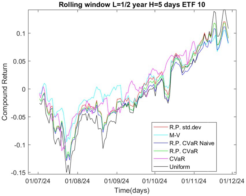
Figure 1. The out-of-sample performance of portfolios composed of 10 stocks.

Figure 1 illustrates the compound return of different portfolio optimization strategies over time, using a rolling window approach for the portfolios composed by 10 stocks. Strategies like Risk Parity CVaR and Risk Parity CVaR Naive may have smoother compound return curves since they are intended to reduce tail risk and deliver more steady performance during market downturns. The M-V approach may exhibit increased unpredictability in compound returns because it is susceptible to changes in expected returns and variances, which can shift dramatically over short periods of time. The Risk Parity with standard deviation strategy, which focuses on distributing risk across assets, may provide a balanced compound return profile. The rolling window technique guarantees that the compound return represents the most recent 6 months’ performance, which is updated every 5 days. This helps to capture the changing nature of the market and the flexibility of each approach.

The Risk Parity CVaR strategy might outperform others during periods of high market volatility, as it explicitly accounts for tail risk. The M-V strategy could outperform during stable or bullish market conditions, where mean and variance estimates are more reliable. The Risk Parity CVaR Naive strategy might underperform compared to the refined Risk Parity CVaR approach, especially during extreme market events. The uniform strategy will have no transaction cost but also more drawdown.

We assume a transaction cost threshold of $\epsilon$ = 0.0001 to ponder as a significant difference between the weights in order to apply the turnover. The level of variable cost is $\alpha =$1% and for fixed cost we assume a flat structure $\gamma =20$ USD according to Lyons (15). By considering a volume of trade is V = 10,000 USD.

Figure 2 highlights the trade-offs between different strategies in terms of transaction costs, which is crucial for portfolio optimization for 3 levels of tolerance of the threshold. The data provided represents the total cost for different portfolio optimization strategies under varying values of ε (epsilon), which acts as a tolerance level in the model. The strategies include Risk Parity with Standard Deviation (RP-Std), Mean–Variance Optimization (M-V), Risk Parity with Conditional Value-at-Risk (RP-CVaR) in both naive and refined forms, and standalone Conditional Value-at-Risk (CVaR).

Figure 2

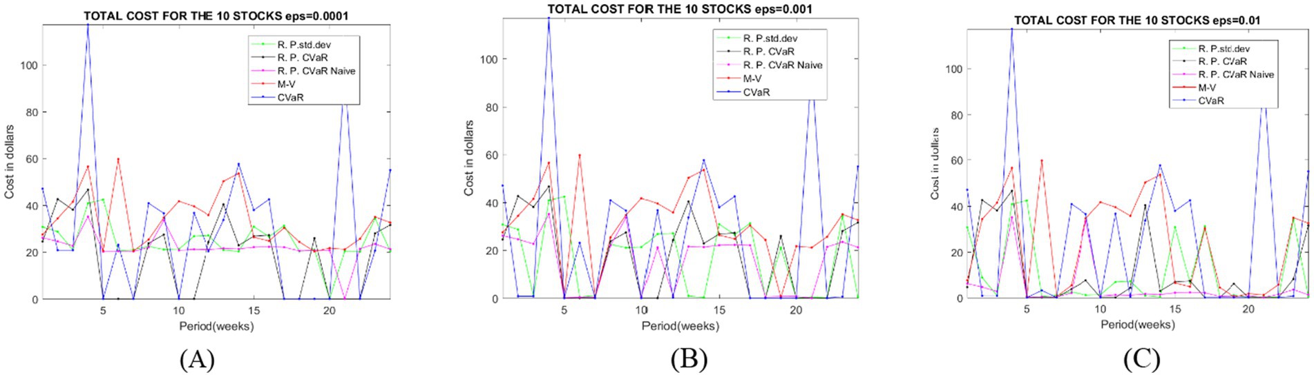
Figure 2. The cost for increasing the level of tolerance. (A) ε =0.0001, (B) ε =0.001, (C) ε =0.01.

In Table 2, as ε increases from 0.00001 to 0.01, the total cost generally decreases for most strategies, indicating that larger values of ε lead to more cost-efficient outcomes. For instance, Risk Parity with standard deviation decreases from 609.63 to 249.63, M-V decreases from 802.53 to 582.53, and Risk Parity CVaR Naive shows a significant drop from 544.37 to 104.37. However, Risk Parity CVaR remains constant at 429.48 for ε = 0.00001 and ε = 0.001, before decreasing to 249.48 at ε = 0.01, while CVaR decreases slightly from 747.13 to 607.13. The Risk Parity CVaR Naive strategy demonstrates the most dramatic reduction in total cost, making it the most sensitive to changes in ε and potentially the most efficient at higher ε values. This analysis highlights the impact of ε on optimization outcomes and helps in identifying the most cost-effective strategies under different conditions. If we change the threshold $\epsilon =0.01$ for the tolerance, it will less cost for the Risk Parity strategies, especially for the Risk Parity Naïve will have even less transaction costs.

Table 2

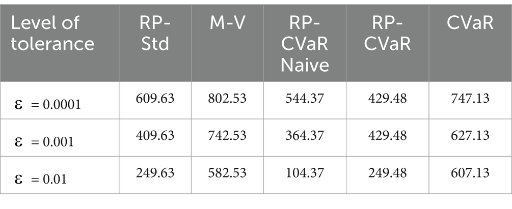
Table 2. The total cost for each level of $\epsilon .$

3.2 The case of a portfolio only with cryptocurrencies

For the second case we choose a portfolio composed by cryptocurrency only. The interval of data is for 1 year, but we have to remind that the crypto market is always opened.

We select from March 7, 2024 to February 20, 2025 for a total of 348 observation. The following Table 3 gives the list of the 10 cryptocurrencies from the whom we are going to create our portfolios. Cryptos are interesting to be studied since they have higher volatility.

Table 3

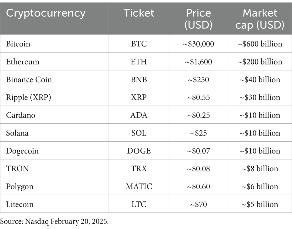
Table 3. The list of cryptocurrencies selected, their ticket, average price and market cap.

We use the data of half of 1 year as an in-sample period L = 182 and holding period L = 6 days with a total of 27 iterations. The following Figure 3 gives the performance in terms of compound returns.

Figure 3

Figure 3. The out-of-sample performance of portfolios composed by cryptocurrencies.

Figure 3 illustrates the compound return of various portfolio optimization strategies applied to a portfolio of 10 cryptocurrencies over time. The graph shows how the compound return of each strategy evolves over time, reflecting the dynamic performance of the cryptocurrency portfolio under different market conditions. Strategies like Risk Parity CVaR and Risk Parity Naive may exhibit smoother compound return curves, as they are designed to mitigate tail risk and provide more stable performance during market downturns. The M-V strategy might show higher variability in compound returns, as it is sensitive to changes in expected returns and variances, which can fluctuate significantly in the volatile cryptocurrency market. The Uniform strategy serves as a baseline and may underperform more sophisticated strategies, especially during periods of high volatility.

The transaction cost the Fixed Costs are rare in most cryptocurrencies, except for XRP and Stellar, which have minimal fixed fees. Variable Costs: Depend on network congestion, transaction size, and blockchain used. For that we consider the level of variable cost is $\alpha =$1% and for fixed cost we assume a flat structure $\gamma =50$ USD, which can be the subscription to the trading platforms. As in the previous case the volume of trade id V = 10,000 USD.

In Figure 4A, for the lowest level of tolerance $\epsilon$  = 0.0001, all curves are relatively flat but high but Mean Variance shows the steepest spikes. For $\epsilon$  = 0.001, Figure 4B, Risk Parity CVaR curve begins to separate from Risk Parity with standard deviation/Risk Parity CVaR Naive, trending downward. Mean Variance cost decreases but remains pronounced. These two are very similar with each other.

Figure 4

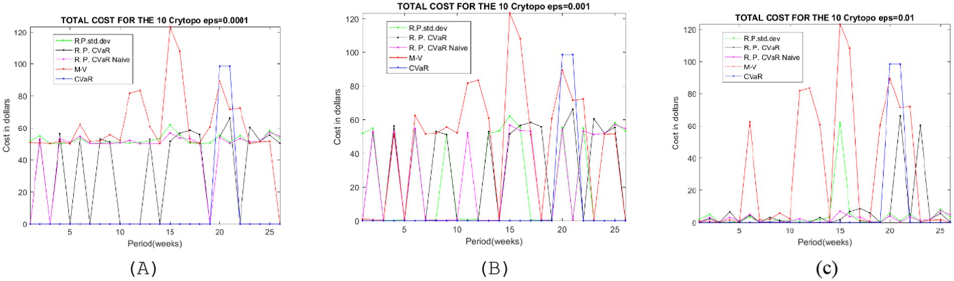
Figure 4. The cost for increasing the level of tolerance. (A) ε =0.0001, (B) ε =0.001, (C) ε =0.01.

In Figure 4C, with the highest level of tolerance $\epsilon$  = 0.01, the total cost decreases significant for all risk parity strategies, reaching the smallest value for Risk Parity with CVaR Naïve (also in Table 4). The weights selected with CVaR, almost unchanged in all three levels of tolerance, showing the same total cost.

Table 4

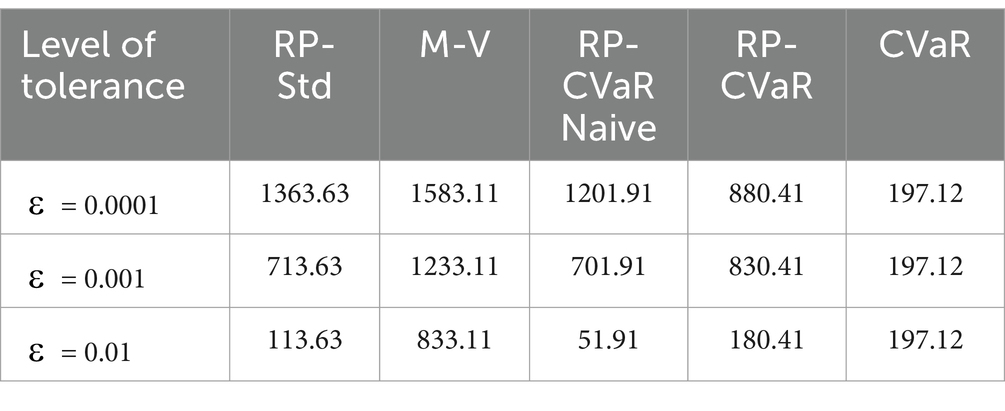
Table 4. The total cost for each level of $\epsilon$ in case of cryptos.

For a better understanding we sum all the total cost for each level of tolerance, given in Table 4.

Mean Variance (M-V) has higher costs than Risk Parity with standard deviation across all ε values, indicating that standard deviation-based risk parity is more efficient than mean–variance optimization in this context. The CVaR strategy consistently yields the lowest cost (197.12) across all ε values, suggesting it is the most robust or conservative approach. This implies that CVaR optimization effectively minimizes tail risk regardless of the risk tolerance level. For most methods (except CVaR), increasing ε (allowing more risk) reduces the cost.

4 Conclusion

This study has explored the impact of transaction costs on the construction and management of minimum risk portfolios, with a particular focus on risk parity models. By incorporating both fixed and variable transaction costs into the optimization framework, we have demonstrated how these costs can significantly affect portfolio performance, particularly in the context of frequent rebalancing and dynamic market conditions. Our empirical investigation, which included both standard stock portfolios and cryptocurrency portfolios, emphasizes the trade-offs between different optimization algorithms as well as the need of taking transaction costs into account while managing a portfolio.

Transaction costs can significantly affect net returns, especially for methods requiring regular rebalancing, such as mean–variance optimization (M-V). Ignoring these costs might result in inefficient asset allocation and higher tracking error, reducing the efficacy of the portfolio strategy.

Risk parity strategies, particularly those that use Conditional Value at Risk (CVaR), offer more consistent performance, particularly during periods of significant market volatility. These models are intended to reduce tail risk and offer more evenly distributed risk contributions across assets, making them more robust to market downturns.

The degree of tolerance for weight modifications is significant in calculating transaction costs. Higher tolerance levels often result in reduced transaction costs since fewer deals are conducted. However, this must be evaluated against the possibility of increased tracking inaccuracy or departure from the targeted risk profile.

Cryptocurrencies, with their extreme volatility and distinctive transaction cost structures, pose new obstacles to portfolio optimization. Our study demonstrates that risk parity methods, particularly those based on CVaR, can be helpful in controlling the inherent hazards of cryptocurrency markets while keeping transaction costs relatively low.

The findings emphasize that while Risk Parity methods are effective in both asset classes, their implementation must account for market-specific traits. Equities benefit from moderate rebalancing tolerance and RP-CVaR, whereas cryptocurrencies demand dynamic adjustments, with RP-CVaR Naïve or pure CVaR being preferable. This comparative analysis underscores that transaction costs and volatility regimes are critical in determining the optimal portfolio strategy, necessitating tailored approaches for equities versus cryptocurrencies.

While this study provides valuable insights into transaction cost-aware portfolio optimization, several limitations must be acknowledged to guide future research. The analysis assumes fixed transaction costs and a uniform trade volume of $10,000, which may not reflect real-world variability in execution costs or liquidity constraints. In practice, transaction costs are dynamic and depend on factors like bid-ask spreads, market impact, and asset liquidity—especially critical for cryptocurrencies, where slippage and thin order books can significantly alter execution costs. The fixed-volume assumption also overlooks whether markets can absorb such trades without adverse price movements. Future work should incorporate: (1) sensitivity analysis to test how varying cost levels and trade volumes affect strategy performance, (2) liquidity-adjusted models that account for bid-ask spreads and execution feasibility, and (3) dynamic cost frameworks that adapt to market depth and volatility regimes. Addressing these gaps would strengthen the practical applicability of the findings, particularly for high-frequency rebalancing or large-scale portfolios where execution costs dominate returns.

Data availability statement

The datasets presented in this study can be found in online repositories. The names of the repository/repositories and accession number(s) can be found in the article/supplementary material.

Author contributions

DV: Conceptualization, Data curation, Funding acquisition, Investigation, Methodology, Resources, Software, Visualization, Writing – original draft, Writing – review & editing. AS: Data curation, Investigation, Methodology, Resources, Supervision, Validation, Visualization, Writing – review & editing. AM: Conceptualization, Data curation, Formal analysis, Investigation, Methodology, Project administration, Software, Supervision, Validation, Visualization, Writing – review & editing.

Funding

The author(s) declare that no financial support was received for the research and/or publication of this article.

Conflict of interest

The authors declare that the research was conducted in the absence of any commercial or financial relationships that could be construed as a potential conflict of interest.

Generative AI statement

The author(s) declare that no Gen AI was used in the creation of this manuscript.

Publisher’s note

All claims expressed in this article are solely those of the authors and do not necessarily represent those of their affiliated organizations, or those of the publisher, the editors and the reviewers. Any product that may be evaluated in this article, or claim that may be made by its manufacturer, is not guaranteed or endorsed by the publisher.

References

1. Olivares-Nadal, AV, and DeMiguel, V. A robust perspective on transaction costs in portfolio optimization. Oper Res. (2018) 66:733–9. doi: 10.1287/opre.2017.1699

PubMed Abstract | Crossref Full Text | Google Scholar

2. Libman, D, Haber, S, and Schaps, M. Forecasting quoted depth with the limit order book. Front Artif Intell. (2021) 4:667780. doi: 10.3389/frai.2021.667780

PubMed Abstract | Crossref Full Text | Google Scholar

3. Ledoit, O, and Wolf, M. Markowitz portfolios under transaction costs. Q Rev Econ Finan. (2025) 100:101962. doi: 10.1016/j.qref.2025.101962

Crossref Full Text | Google Scholar

4. Yoshimoto, A. The mean-variance approach to portfolio optimization subject to transaction costs. J Oper Res Soc Jpn. (1996) 39:99–117. doi: 10.15807/jorsj.39.99

Crossref Full Text | Google Scholar

5. Wang, X, Zhu, Y, and Tang, P. Uncertain mean-CVaR model for portfolio selection with transaction cost and investors’ preferences. North Am J Econ Finan. (2024) 69:102028. doi: 10.1016/j.najef.2023.102028

Crossref Full Text | Google Scholar

6. Guo, S, Gu, JW, Ching, WK, and Lyu, B. Adaptive online mean-variance portfolio selection with transaction costs. Quant Financ. (2023) 24:59–82. doi: 10.1080/14697688.2023.2287134

PubMed Abstract | Crossref Full Text | Google Scholar

7. DeMiguel, V, Garlappi, L, Uppal, R, and Diversification, OVN. How inefficient is the 1/N portfolio strategy? Rev Financ Stud. (2009) 22:1915–53. doi: 10.1093/rfs/hhm075

Crossref Full Text | Google Scholar

8. Perold, AF. The implementation shortfall: paper versus reality. J Portf Manag. (1988) 14:4–9. doi: 10.3905/jpm.1988.409150

Crossref Full Text | Google Scholar

9. Lobo, MS, Fazel, M, and Boyd, S. Portfolio optimization with linear and fixed transaction costs. Ann Oper Res. (2007) 152:341–65. doi: 10.1007/s10479-006-0145-1

Crossref Full Text | Google Scholar

10. Best, MJ, and Grauer, RR. On the sensitivity of mean-variance-efficient portfolios to changes in asset means: some analytical and computational results. Rev Financ Stud. (1991) 4:315–42. doi: 10.1093/rfs/4.2.315

Crossref Full Text | Google Scholar

11. Veliu, D, and Aranitasi, M. Small portfolio construction with cryptocurrencies. WSEAS Trans Bus Econ. (2024) 21:686–93. doi: 10.37394/23207.2024.21.57

Crossref Full Text | Google Scholar

12. Acerbi, C, and Tasche, D. On the coherence of expected shortfall. J Bank Financ. (2002) 26:1487–503. doi: 10.1016/S0378-4266(02)00283-2

Crossref Full Text | Google Scholar

13. Stefanovits, David. (2010). "Equal contributions to risk and portfolio construction." ETH Zurich, ethz.ch/content/dam/ethz/special-interest/math/risklab-dam/documents/walter-saxerpreis/ma-stefanovits.pdf (Accessed April 11)

Google Scholar

14. Gârleanu, N, and Pedersen, LH. Dynamic trading with predictable returns and transaction costs. J Financ. (2013) 68:2309–40. doi: 10.1111/jofi.12080

Crossref Full Text | Google Scholar

15. Lyons, RK. The microstructure approach to exchange rates, vol. 333. Cambridge, MA: MIT Press (2001).

Google Scholar