A Hierarchical Archimedean Copula (HAC) model for climatic variables: an application to Kenyan data

Introduction: Advanced statistical modeling techniques, such as copula-based methods, have significantly improved the forecasting of weather variables by capturing dependencies between them. However, conventional copula approaches, such as the bivariate copula, often fail to capture complex interactions in high-dimensional climate data. This study aims to develop a multivariate joint distribution model for climatic variables using the Hierarchical Archimedean Copula (HAC) framework.

Methods: Parametric methods were used to fit marginal distributions to the six variables. The uniform variates were extracted using the inverse transformation technique. The structure and parameter estimation of HAC models were determined using the Recursive Maximum likelihood (RML) method. Model selection methods, Goodness of Fit (GOF) approaches, and graphical assessment were used to select the optimal HAC model.

Results: The Weibull distribution was identified as the best fit for temperature, humidity, solar energy, and cloud cover, while the Gamma distribution was most suitable for wind, and the logistic distribution for sea-level pressure. For high-dimensional data, the HAC Frank copula demonstrated computational efficiency and effectively captured dependencies among variables.

Discussion: The HAC-Frank model offers a reliable and computationally efficient alternative for modeling high-dimensional climate dependencies, thereby providing a robust framework for climate forecasting, risk assessment, and environmental modeling.

1 Introduction

The impact of climate change has been on the upward trend in recent decade, affecting, food security, disaster management, nutritional outcomes, infrastructure, among others [1]. The unfavorable effect of climate change in Kenya has intensified due to over reliance on subsistence farming, which is highly dependent on favorable weather conditions [2]. According to IPCC [3] and Obwocha et al. [4], the adverse effect of climate change is mainly due to interaction of multiple factors, including high temperatures, erratic rainfall patterns, soil erosion, and extreme weather events. To mitigate the effect of climate change, it is imperative to understand the intricate relationships among these weather variables [5–7].

Conventionally, the Pearson correlation coefficient has long been used as a measure of dependence between two variables, based on the assumption that the two variables have a linear relationship [8]. In his research on pitfalls of correlation, Embrechts et al. [9] highlighted a number of fallacies concerning correlation and in his subsequent work, Embrechts et al. [10] provided some alternative measures of correlation and introduced copulas as the best alternative to understand dependence between variables. Over the past three decades, the application of copulas has expanded across various fields resulting in a better understanding of concept of copulas [5, 11–15].

During this period of evolution of copula theory, the primary focus has been on bivariate analysis as used in Chowdhary [5], Cong and Brady [16], Dzupire et al. [17], and Yee et al. [18] for joint modeling of climatic variables. A number of copula functions exist to capture different dependence structures [19]. Among these, Archimedean Copulas (ACs) are notable as one of the most widely used copulas due to their flexibility, symmetry, and associativity properties [16, 18]. In addition, ACs possess different generating functions, making it flexible for capturing diverse dependence structures [20]. Despite over reliance on use of ACs for bivariate analysis, they fall short due to their exchangeability property and reliance on a single parameter for measuring dependence [21]. In this era of big data, to capture dependence for high dimensional data would be problematic if a single parameter is used [22]. Hence, to capture dependence for high dimensional data, researchers have resorted to HAC or vine copulas to ensure flexibility is retained within the bivariate analysis.

Although simple ACs are flexible, HAC models have proven to be more flexible than ACs [15, 23]. The different levels of hierarchy within the HAC models are particularly useful for capturing asymmetries in bivariate dependencies, a task that standard ACs cannot accomplish. Additionally, HAC models provide detailed information about marginal cumulative distribution functions at each node of the hierarchical tree. When a single generator function is applied, these models facilitate simplified dependence analysis across different hierarchical levels, allowing for varying degrees of dependence between variable variables [24–26]. For instance, Grimaldi and Serinaldi [27] and Serinaldi and Grimaldi [28] used a trivariate copula to measure dependence between peak and total depth, conditioned on critical depth. Saad et al. [26] applied a trivariate HAC for hydrometeorological flood analysis. Ribeiro et al. [6] used HAC to examine model dependencies among precipitation, maximum temperature, and crop yields too. Researchers have also used vine copulas for dependence modeling in high-dimensional settings, as demonstrated in studies by Brechmann et al. [29], Czado et al. [11], Joe and Dorota [30], Maina et al. [31], Vernieuwe et al. [32], and Wang et al. [33]. Due to their flexibility, vine copulas can effectively capture both the type and strength of dependence for each pair in a bivariate analysis [30].

Although HAC models have been used for multivariate modeling with more than three variables, their applications vary across different fields. For example, Ma et al. [34] used HAC to evaluate the seismic vulnerability of multispan bridge systems, while Yang et al. [35] used HAC to examine five-dimensional wind and wave data close to a sea-crossing bridge. HAC was also used by Lin-Ye et al. [36] to model the combined distribution of upcoming marine storms. Furthermore, HAC was used by Lin-Ye et al. [25] to investigate wave extreme events throughout the Catalan coast. Despite these applications, there remains a significant gap in the literature regarding the use of HAC models for more than five variables, particularly in climatic contexts involving a broad range of weather variables. This is attributed to multiple dependencies which introduce computational challenges, making parameter estimation, model selection, and validation of nesting conditions increasingly complex. Although HACs have been extensively used in hydrology [8, 24, 26–28] and finance [15, 22, 37, 38], their potential in climate science is still largely unexplored. In addition, asymmetric dependencies are frequently observed in climate variables, which AC models may not adequately represent in higher dimensions. In high-dimensional climate modeling, existing research primarily relies on vine copulas and elliptical copulas, with relatively few studies utilizing HACs. As well, there is a lack of comprehensive comparative analysis that evaluates HACs in the context of high-dimensional climate modeling.

Therefore, we developed a multivariate joint distribution framework to construct a six-dimensional model for climatic variables using HAC approach. The six climatic variables under consideration are temperature, humidity, cloud cover, wind speed, sea level pressure, and solar energy. The focus was on copulas belonging to the same family, following the approach proposed by Okhrin et al. [39] and Okhrin et al. [21] who highlighted the limitations of heterogeneous HAC models in handling high-dimensional data. Our research is unique in its ability to capture dependence of more than five variables and for modeling climatic variables specific to Kenya. After fitting the HAC model, we conducted a comprehensive model selection process and performed GOF tests to identify the optimal HAC structure for these climatic variables. Graphical assessments were also used to assess the consistency and robustness of the integrated approach. Our third goal was to evaluate how well the vine copula and HAC models function in high-dimensional environments, revealing the relative advantages and disadvantages of each in terms of capturing intricate dependency patterns.

2 Materials and methods

2.1 Datasets

The dataset used in the proposed statistical model was obtained from Visual Crossing (VC) [40]. VC aggregates data from several sources with Integrated Surface Database (ISD) of National Oceanic and Atmospheric Administration (NOAA) as one of the primary sources. ISD is a comprehensive database of weather observations collected from weather stations throughout the world on an hourly and sub-hourly basis. The study used recorded daily weather data from the Nairobi Wilson Airport weather station (HKNW), while remotely sensed data from Jomo Kenyatta International Airport (HKJK) were integrated to fill in any missing observations.

The dataset has 36 variables, over a span of 4-year period (January 1, 2020–December 31, 2023). From this dataset, six key variables were selected from this dataset (temperature, humidity, cloud cover, wind speed, sea level pressure, and solar energy) were selected for modeling. These variables were selected because of their proven value in climatic modeling and their ability to capture atmospheric conditions [6, 16, 41]. Their selection aligns with the study's focus on HAC models, which require a structured dependency framework. HAC models are especially well suited for this kind of data because they can capture nonlinear, asymmetric, and tail dependencies [6, 15, 22].

The dataset obtained from VC had already undergone preprocessing and cleaning before further analysis (for more information about preprocessing and data cleaning [40]). The selected variables were transformed before fitting the HAC models using probability density functions, to enhance appropriate representation of data for copula construction.

Temperature (temp), which is expressed in degrees Celsius (°C) in Table 1, represents the daily average obtained from hourly readings taken throughout the day. Humidity, expressed as relative humidity (%), measures the proportion of water vapor in the air relative to its maximum capacity at a given temperature—values below 30% indicate dry conditions, 30%−70% are considered comfortable, while levels above 70% denote humid conditions. Solar energy (solarenergy), expressed in megajoules per square meter (MJ/m²) estimates the overall amount of solar energy that has gathered throughout the day obtained by summing hourly record. Cloud cover (cloudcover) represents the percentage of the sky obscured by clouds, calculated as the mean of hourly cloud cover observations across different altitudes. To ensure comparability across different locations, sea level pressure (pressure), which is measured in millibars (mb), is an adjustment of atmospheric pressure that eliminates the effects of elevation. Lastly, wind speed (windspeed), typically recorded in kilometers per hour (km/h), reflects the average air movement over a 2-min period before logging. To maintain consistency, wind speed measurements are standardized at a height of 10 meters above ground in open areas to minimize interference from surrounding obstacles.

Table 1

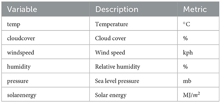
Table 1. List of the weather variables.

2.2 Copula theory

A copula is a mathematical function that connects two or more variables, facilitating the modeling of their joint behavior while preserving their individual marginal distributions [19, 42]. Each variable follows its own distinct distribution pattern, known as the marginal distribution.

Definition (Copula)

A function C:[0, 1]^d → [0, 1] is called a d-dimensional copula if there exist a probability space (Ω, Σ, P) and a random vector U∈[0, 1]^d such that:

$\begin{array}{ll}P(U_j\le u_j)=u_j,\text{\hspace{1em}for every }{u}_j\in [0,1],\text{ and\hspace{1em}}j=1,2,\mathrm{...},d& (1)\end{array}$

and:

$\begin{array}{l}C(u_1,\mathrm{...},u_d)=P(U_1\le u_1,\mathrm{...},U_d\le u_d),\text{\hspace{1em}for every }{[u_1,\mathrm{...},u_d]}^T\\ \in {[0,1]}^d.& (2)\end{array}$

The function C is a copula. If F_i(X_i) represents the marginal distributions, then the function:

$\begin{array}{ll}C(F_1(X_1),F_2(X_2),\mathrm{...},F_d(X_d))=F(x_1,\mathrm{...},x_d)& (3)\end{array}$

defines a multivariate distribution for the random variables X₁, ..., X_d.

Consider a 6-variate case, X₁, X₂, ..., X₆, with marginal distribution functions F₁(x₁), F₂(x₂), ..., F₆(x₆), respectively. We are interested in obtaining a joint cumulative distribution function F(X₁, X₂, ..., X₆) with these marginals. Sklar [42] demonstrated that there always exists a function C such that:

$\begin{array}{ll}F(X_1\le x_1,X_2\le x_2,\mathrm{...},X_6\le x_6)=C(F_1(X_1),F_2(X_2),\mathrm{...},F_6(X_6)).& (4)\end{array}$

Or equivalently:

$\begin{array}{ll}F(F_1^{-1}(u_1),F_2^{-1}(u_2),\mathrm{...},F_6^{-1}(u_6))=C(u_1,\mathrm{...},u_6),& (5)\end{array}$

where $F_i^{-1}(u_i)$ are the inverse functions of the marginal cumulative distribution functions (CDFs) and the joint probability density function (PDF) for continuous margins is:

$\begin{array}{ll}f(x_1,\mathrm{...},x_6)=c(u_1,\mathrm{...},u_6)f_1(x_1)f_2(x_2)\mathrm{...}{f}_6(x_6).& (6)\end{array}$

The copula density c(u₁, ..., u₆) is derived by differentiating Equation 3 as follows:

$\begin{array}{ll}c(u_1,\mathrm{...},u_6)=\frac{{\partial }^{6}C(u_1,\mathrm{...},u_6)}{\partial u_1\partial u_2\partial u_3\partial u_4\partial u_5\partial u_6}.& (7)\end{array}$

2.2.1 Hierarchical Archimedean copula

Unlike other copulas, such as elliptical copulas, ACs are not constructed using Sklar's theorem. Instead, they rely on a specific functional form and properties necessary to obtain a valid copula [43]. According to McNeil and Nešlehová [44] a multivariate ACs that is exchangeable is defined by:

$\begin{array}{ll}C(u_1,\mathrm{...},u_d)=\phi \left({\phi }^{-1}(u_1)+{\phi }^{-1}(u_2)+\mathrm{...}+{\phi }^{-1}(u_d)\right),& (8)\end{array}$

where φ:[0, ∞) → [0, 1], known as the generator, is any continuous, decreasing, convex function satisfying φ(0) = 1, φ(∞) = 0. Kimberling [45] and McNeil and Nešlehová [44] demonstrated that the copula generated by the generator φ, a completely monotonic function, must also satisfy the following condition for its pseudo-inverse:

$\begin{array}{ll}{(-1)}^k\frac{{\partial }^k}{\partial u^k}{\phi }^{-1}(u)\ge 0,u>0,k\in \mathbb{N}.& (9)\end{array}$

The generator function φ provides different types of ACs as noted by Nelsen [19] and Okhrin et al. [43].

A list of AC generators for the various types of ACs used in this study is provided in Table 2. According to Chowdhary [5], Cong and Brady [16], and Mallick et al. [7], ACs are well known for their adaptability in simulating both positive and negative dependence structures. In addition, they have straightforward closed-form representations, which makes them effective for estimating parameter [24]. By employing a single function, ACs can capture both lower and upper tail dependencies, making them particularly useful for modeling extreme events [18]. Because they assume symmetric dependence structures, which might not necessarily reflect asymmetric dependencies, they are unduly limiting for some applications due to their single dependence parameter [21, 46]. Furthermore, Hofert and Mächler [47] highlighted that ACs are problematic when extended to include more relationships involving more than two variables. To address this challenge [20] proposed the concept of HACs among other approaches. The benefits of HAC are summarized in Yang et al. [35].

Table 2

Table 2. Description of the generating functions, parameter constraints as well as of the relationships between Copula parameter and Kendall's tau.

2.2.2 Vine Copula

According to Joe and Dorota [30], vines are graphical structures that represent joint probability distributions. The joint probability distributions are decomposed into bivariate copulas known as pair copulas [48]. If you consider a d dimensional data, $\frac{d(d-1)}{2}$ pairs of copulas can be constructed as building blocks in a hierarchical framework [30, 49–51]. A wide range of bivariate copulas as shown in Joe et al. [20] and Nelsen [19] can be used to capture dependence at different hierarchical levels, providing flexibility unlike the HAC models, which rely solely on ACs. This approach has been successfully applied in finance [11, 29, 51] and in climate [32, 33, 41], to mention a few. In this work, vine copula was used for comparison with HAC model in terms of performance for the climate data.

2.2.3 General HAC framework

HACs are constructed step by step through the combination of simple ACs into more complex structures [20, 39]. Instead of modeling just two variables in terms of dependence structures, this approach allows for extensions to three, four, or more variables by nesting smaller ACs within larger ones. ACs are used to connect variable pairs at the lowest hierarchical level and a parameter for the pairs is estimated. The couple with the strongest dependence is aggregated and replaced by a joint pseudo-variable [39]. At the next hierarchy level, another AC is applied to model the dependence between the resulting pairs of variables. This process continues iteratively until all variables are interconnected. During this procedure, it is essential to verify that a proper copula results from the grouping by ensuring the sufficient nesting condition is met (see Lemma 4.1 in McNeil [52]). The general form of a d- dimensional HAC structure may be defined as follows:

$\begin{array}{l}{\phi }_{{\theta }_{d-1}}\{{\phi }_{{\theta }_{d-1}}^{[-1]}(u_d)+{\phi }_{{\theta }_{d-1}}^{[-1]}⚬C_{d-1}(u_1,\dots ,u_{d-1};s_{d-2},({\theta }_1,\dots ,\\ {{\theta }_{d-2})}^T)\}, & (10)\end{array}$

where $\theta ={({\theta }_1,\dots ,{\theta }_{d-2})}^T$ represents the parameter vector of the HAC and s denotes the structure of the HAC [15]. For example, special case for a fully nested and partially HAC for d = 6 can be illustrated together in Figure 1. For fully nested HAC, the copula function in Equation 10 is given by

$\begin{array}{l}C(u_1,u_2,u_3,u_4,u_5,u_6)=\\ C_6\left\{C_5\left(C_4\left(C_3\left(C_2(u_1,u_2),u_3\right),u_4\right),u_5\right),u_6\right\},& (11)\end{array}$

$\begin{array}{l}C(u_1,u_2,u_3,u_4,u_5,u_6)=\\ {\phi }_6\{{\phi }_6^{-1}⚬{\phi }_5[{\phi }_5^{-1}⚬{\phi }_4({\phi }_4^{-1}⚬{\phi }_3({\phi }_3^{-1}⚬{\phi }_2({\phi }_2^{-1}(u_1)+{\phi }_2^{-1}(u_2))\\ +{\phi }_3^{-1}(u_3))+{\phi }_4^{-1}(u_4))+{\phi }_5^{-1}(u_5)]+{\phi }_6^{-1}(u_6)\},& (12)\end{array}$

which simplifies to:

$\begin{array}{ll}C(u_1,u_2,u_3,u_4,u_5,u_6;s=\left(\left(\left(\left(\left(12\right)3\right)4\right)5\right)6\right),\theta ={\left({\theta }_1,{\theta }_2,{\theta }_3,{\theta }_4,{\theta }_5\right)}^T).& (13)\end{array}$

For a partially nested HAC, Equation 10 can also be expressed as:

$\begin{array}{l}C(u_1,u_2,u_3,u_4,u_5,u_6)=C_6\{C_5\left(C_4(u_1,u_2),u_3\right),C_3(C_2(u_4,u_5),\\ u_6)\}, & (14)\end{array}$

$\begin{array}{l}C(u_1,u_2,u_3,u_4,u_5,u_6)=\\ {\phi }_6\{{\phi }_6^{-1}⚬{\phi }_5\left[{\phi }_5^{-1}⚬{\phi }_4\left({\phi }_4^{-1}(u_1)+{\phi }_4^{-1}(u_2)\right)+{\phi }_5^{-1}(u_3)\right]\\ +{\phi }_6^{-1}⚬{\phi }_3\left[{\phi }_3^{-1}⚬{\phi }_2\left({\phi }_2^{-1}(u_4)+{\phi }_2^{-1}(u_5)\right)+{\phi }_3^{-1}(u_6)\right]\},& (15)\end{array}$

$\begin{array}{ll}C(u_1,u_2,u_3,u_4,u_5,u_6;s=(((12)3)((45)6)),\theta ={({\theta }_1,{\theta }_2,{\theta }_3,{\theta }_4,{\theta }_5)}^T).& (16)\end{array}$

Note that the copula function on Equation 10 can take different forms of HAC structures. The function in Equations 12, 15 are just one of the many possible binary structures that can be created.

Figure 1

Figure 1. Fully and partially nested HAC of dimension d = 6 with structures s = ((((12)3)4)5)6 on the left and s = (((12)3)((45)6)) on the right.

2.3 HAC estimation

In this section, we describe the HAC estimation procedure, which is divided into three parts. The first part involves the estimation of marginal distributions using the six variables. We also describe the GOF tests conducted to determine the best-fitting probability distributions and apply the inverse transformation method to extract pseudo-observations. The second part focuses on the estimation of the HAC structure and parameters using the RML approach. Finally, the third section addresses model selection and evaluation. A flowchart in Figure 2 provides a summary of the methodology adopted in this paper.

Figure 2

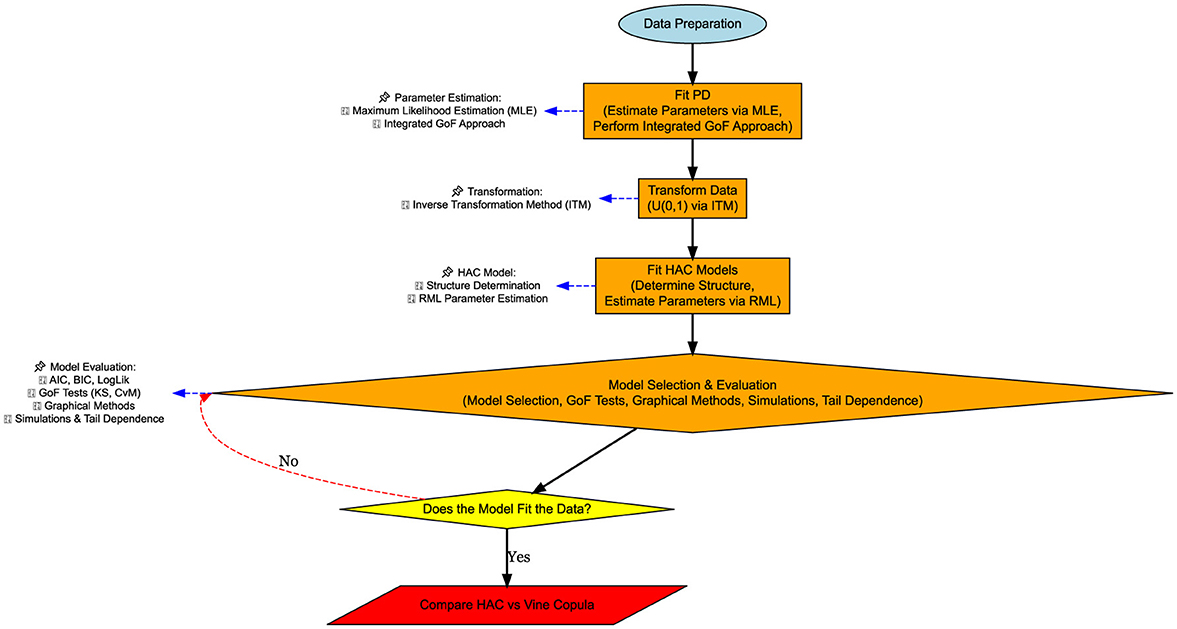
Figure 2. Step-by-step flowchart of the methodology: fitting probability distribution, HAC model selection, parameter estimation, and validation.

2.3.1 Marginal distributions

To extract uniform random variables, a parametric method was employed in this study. Among the six selected variables, seven common univariate probability distributions were tested to fit the data [53]. The PDFs and associated parameters are summarized in Table 3 as described by Naghettini [54]. A comprehensive approach was used to select the fitting distribution [5, 55]. To ensure a robust choice of the best probability distribution model, this approach integrated graphical analysis, information criteria, and several GOF tests. Each distribution model is put through multiple GOF tests, and the model that performs the best in each test is awarded the highest score. Each model is ranked independently for each GOF test before being aggregated together for all tests to create a composite score. For graphical assessments, rankings are informed by visual inspection of density plots and quantile-quantile (Q-Q) plots, providing additional insight into the best-fitting model.

Table 3

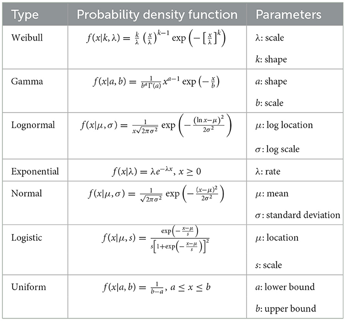
Table 3. Univariate probability distributions and their parameters.

2.3.2 HAC structure and parameter estimation

Numerous studies have examined the process of estimating parameters and structures of HAC [21, 39, 43, 46]. When constructing HACs, the copulas can belong to the same family or to different families, referred to as homogeneous and heterogeneous HACs, respectively [21]. McNeil [52] provided a framework to guarantee that the nested copulas produce a valid copula satisfying sufficient nesting conditions (SNC). While SNC are always guaranteed for homogeneous HACs [39], it may not always be the case for heterogeneous HACs [47]. In this paper, we adopted homogeneous HACs for the HAC structure and parameter estimation using the recursive maximum likelihood (RML) approach proposed by Okhrin et al. [39]. The algorithm proceeds as follows:

1. Fit bivariate copulas to every pair of variables. In this case, we fitted $\genfrac{}{}{0.0pt}{}{6}{2}=15$ AC models for each copula function provided in Table 2. The pair with the strongest dependency, denoted as l₁, is selected along with its parameter estimate $\widehat{{\theta }_1}$.

2. Form a pseudo-variable $Z_1=C(l_1,{\phi }_1;\widehat{{\theta }_1})$, which represents the joint dependency of the selected pair.

3. Repeat step 1 using the new pseudo-variable Z₁ and the remaining variables.

4. Determine the set of variables with the best fit at the second level.

5. Create a new pseudo-variable $Z_2=C(l_2,{\phi }_2;\widehat{{\theta }_2})$, combining the two variables.

6. Continue this procedure until only one variable remains d_j = 1.

At the first stage of estimation, copula parameters are initialized from known marginal distributions. In subsequent stages, the parameters are refined by assuming the marginals and copula families at lower levels are known. Let $X={\left\{x_{ij}\right\}}^T$ be our sample of size n for i = 1, …, n, j = 1, …, d. If we assume d variables are joined by p nested levels, let $\alpha ={(\widehat{{\alpha }_1},\dots ,\widehat{{\alpha }_d})}^T$ denote the vector of parameters of marginal distributions and $\theta ={(\widehat{{\theta }_1},\dots ,\widehat{{\theta }_{d-1}})}^T$ are parameters of the copula starting with the smallest to the largest value. The RML for $\widehat{\beta }$ of $\beta =(\widehat{\alpha },\widehat{\theta })$ with parametric margins is given by:

$\begin{array}{l}l(\beta ,X)={\displaystyle \sum _{i=1}^n\log }[c(\phi ,\theta ,s)\left(F_1(x_{1i},{\alpha }_1),\dots ,F_d(x_{di},{\alpha }_d)\right){\displaystyle \prod _{j=1}^d}\\ f_j(x_{ji},{\alpha }_j)],& (17)\end{array}$

$\begin{array}{l}={\displaystyle \sum _{i=1}^n[\log c(\phi ,\theta ,s)\left(F_1(x_{1i},{\alpha }_1),\dots ,F_d(x_{di},{\alpha }_d)\right)}\\ +{\displaystyle \sum _{i=1}^d\log }{f}_j(x_{ji},{\alpha }_j)].& (18)\end{array}$

The recursive ML approach solves the system and obtains the estimators by solving the following equations:

$\begin{array}{ll}{\left[\frac{\partial l_1}{\partial {\alpha }_1^{\prime }},\dots ,\frac{\partial l_d}{\partial {\alpha }_d^{\prime }},\dots ,\frac{\partial l_1}{\partial {\theta }_1^{\prime }},\dots ,\frac{\partial l_{d-1}}{\partial {\theta }_{d-1}^{\prime }}\right]}^T=0.& (19)\end{array}$

where j = 1, …, d−1, and the process continues for the five copula families mentioned in Table 2.

2.3.2.1 Assumptions

The construction of HAC model was based on several assumptions that guarantees the validity of the HAC model. Firstly, it was assumed that the marginal distributions are correctly specified [20]. In this study, the marginal distributions were first estimated before proceeding with HAC modeling. In instances where margins were not explicitly specified or were uncertain, a non-parametric approach should be employed to estimate them. Secondly, each copula within the HAC model was assumed to have a generating function that is completely monotonic, ensuring the proper construction of the hierarchical dependence structure. Thirdly, to maintain the consistency across the nested structure, all generator functions must belong to the same family. Furthermore, the estimated parameters must satisfy the nesting condition, meaning that the dependence parameter of the parent copula must be greater than or equal to that of the child copula θ_parent≥θ_child. To preserve the hierarchical structure of the model, the lower-level dependencies must be stronger than those at higher levels. Finally, it is important to note that ACs in HAC models are non-exchangeable, meaning that the order of variables affects the dependence structure, differentiating them from elliptical copulas. For further details on HAC model assumptions, see Okhrin et al. [21, 23, 39].

2.4 Model selection and goodness of fit tests

2.4.1 Model selection

Model selection techniques such as AIC, BIC, and log-likelihood (loglik) were evaluated in order to choose the optimal model. The model with the highest loglik, or the lowest AIC or BIC, was selected as the best fit [16, 31, 54, 56]. AIC and BIC are defined as follows:

$\begin{array}{ll}AIC=-2\log lik+2p,& (20)\\ BIC=-2\log lik+p\log (n),& (21)\end{array}$

where n is the sample size and p represents the number of generators or copula parameters [35, 57].

2.4.2 Goodness of fit tests

Once the best model was selected, GOF tests were performed to evaluate how well the chosen model fits the data. The empirical copula values for the variables are compared against the theoretical values to assess accuracy.

The empirical copula P_e(i) for the six variables is computed as follows:

$\begin{array}{ll}{P}_e(i)=\widehat{C}(u_1,u_2,u_3,u_4,u_5,u_6)=n^{-1}{\displaystyle \sum _{i=1}^n{\displaystyle \prod _{j=1}^{d}I}}\left\{\widehat{F_j}(x_{ij})\le u_j\right\},& (22)\end{array}$

where $\widehat{F_j}(x_{ij})$ denotes the estimated marginal distribution of variable x_j and I is the indicator function [58, 59]. Metrics such as the root mean square error (RMSE), CVM $(S_n^{(E)})$, and KS tests D_n were computed as follows:

$\begin{array}{ll}\text{RMSE}=\sqrt{n^{-1}{\displaystyle \sum _{i=1}^n{\left[P_e(i)-P_c(i)\right]}^2}},& (23)\end{array}$

$\begin{array}{ll}{S}_n^{(E)}={\displaystyle \sum _{i=1}^n{\left[P_e(i)-P_c(i)\right]}^2},& (24)\end{array}$

$\begin{array}{ll}{D}_n=\underset{x}{\max }|P_e(i)-P_c(i)|.& (25)\end{array}$

Additionally, graphical tools such as Q–Q plots was used to assess the closeness between the HAC model and empirical HAC and Kendall's tau was employed to evaluate the strength of association between simulated HAC models and the observed data for the six variables [56, 60].

Modified Wasserstein distance (WD) statistic was used to compare the HAC model and the vine copula model. This was applied in addition to the GOF tests described above. The (WD) is a metric used to measure the discrepancy between two probability distributions [61–63]. The modified (WD) between two CDFs, F(x) and G(x) is given by:

$\begin{array}{ll}{W}_1\left(F,G\right)={\displaystyle {\int }_{-\infty }^{+\infty }\left|F\left(x\right)-G\left(x\right)\right|}dx.& (26)\end{array}$

where F(x) represents the empirical CDF and G(x) is the theoretical CDF derived from the HAC or vine copula model. A better fit shows similarity between the two distributions and it is determined by a lower W₁(F, G) value.

3 Results

3.1 Description of the variables

A total of 1, 461 observations that spans over 4 years was used to extract summary statistics in Table 4a. The findings show that the six climatic variables exhibit diverse distributions. Temperature has a narrow range (15.00−−23.90°C) with low variability (SD = 1.61) and a slight negative skewness (−0.26). Humidity shows moderate variability (SD = 9.78) with a wider range (38.50−−96.40%) and a nearly symmetric distribution (skew = −0.28). Solar energy has a range of 4.60−−31.90 MJ/m² and moderate variability (SD = 5.27), with a slight negative skewness (−0.31). Cloud cover demonstrates the highest variability (SD = 15.49) and a negative skewness (−1.22), indicating frequent higher cloud coverage. Sea level pressure, ranging from 1,012.60 to 1,028.40 mb, had low variability (SD = 2.06) and was nearly symmetric (skew = −0.16). Wind speed had a very wide range 9.40−−183.60 (km/h) with significant variability (SD = 8.87), an extreme positive skewness (7.44), and highly leptokurtic (113.67), suggesting occasional extreme wind events. The first five variables share characteristics of negative skewness and platykurtosis, indicating flatter distributions with slightly left-tailed tendencies.

Table 4

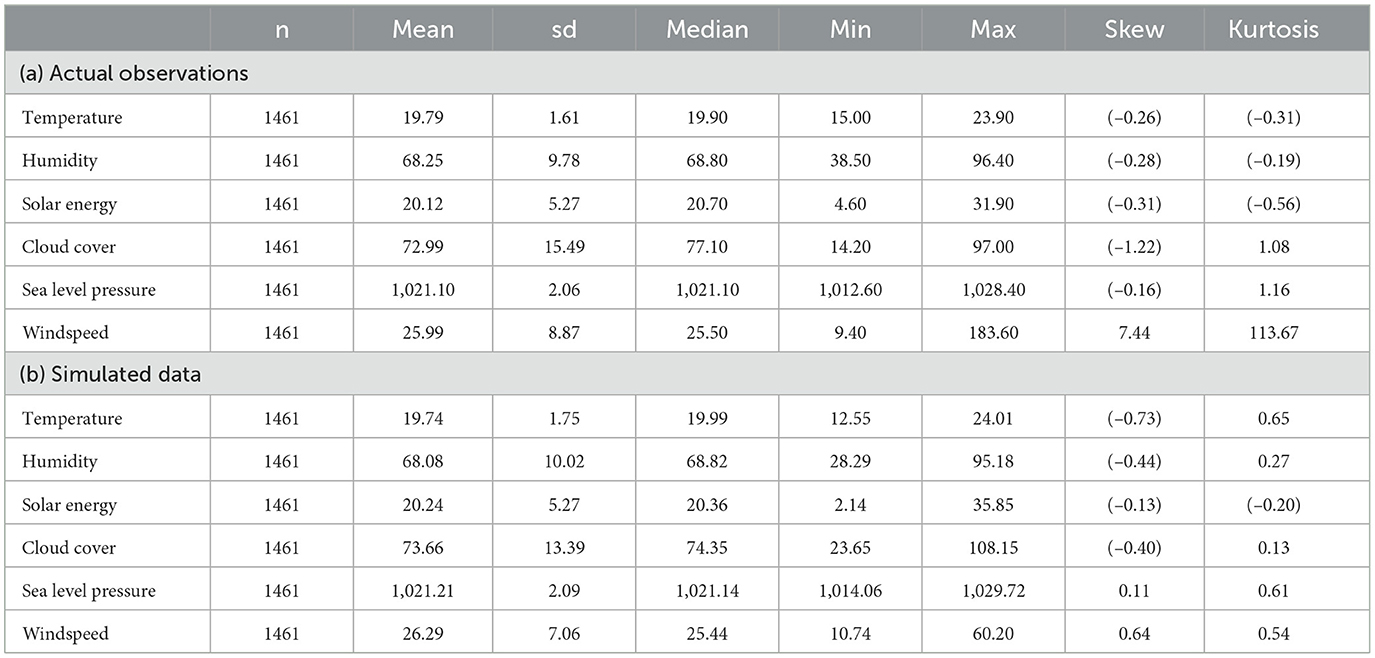
Table 4. Summary statistics for the six variables: (a) actual data and (b) simulated data.

3.2 Correlational analysis

Correlation plots were used to assess the dependence between pairs of the six variables, as shown in Figure 3. The correlation matrix highlights strong correlations among several variable pairs. Notably, solar energy and temperature had a strong positive correlation (r = 0.710), while temperature demonstrates strong negative correlations with humidity (r = −0.588) and cloud cover (r = −0.528). Weak correlation was observed between sea level pressure and humidity (r = 0.110), indicating weaker linear relationship. A similar conclusion was seen between wind speed and solar energy (r = −0.170). Most of the variables had a positive and negative correlation coefficient between r = (0.3 − 0.6) that shows a variety of weak to moderate dependencies between the six climatic variables.

Figure 3

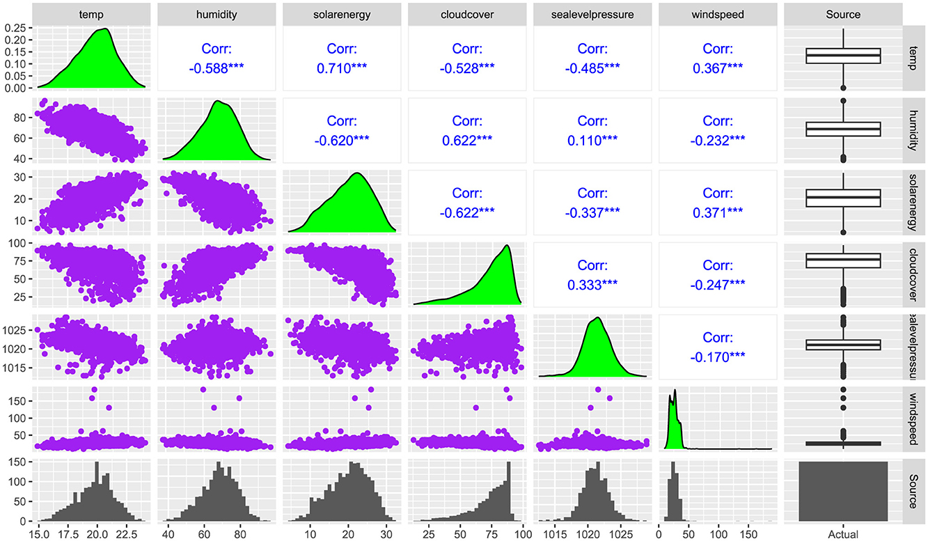
Figure 3. A combination of scatter plots (Purple), Density plots (Green) Spearman Rank correlation coefficients (Blue), Histogram (Bottom – Light gray), and Boxplots (Right – Light gray) for Temperature, Humidity, Solar energy, Cloud cover, Sea level pressure, and Windspeed. The *** means significance level at 1%.

3.3 Marginal distributions

The maximum likelihood estimation approach (MLE) was used to fit the probability distributions to the six variables. The results for each variable are presented in Table 5. The graphical assessments and the results of GOF test in Table 5a shows that the Weibull distribution consistently provided the best fit for temperature, humidity, solar energy, and cloud cover across all GOF tests, including the KS, AD, CVM, and chi-squared (CHI) tests, as well as density and Q-Q plots. The sea-level pressure was best modeled using the logistic distribution, which performed well in most evaluation criteria. For wind speed, the lognormal distribution exhibited strong performance across most tests. The parameter estimates in Table 5b were obtained from the best-fitting probability distributions. Then, the inverse transformation method was applied using these estimates to generate empirical cumulative distribution functions (ECDFs) with uniform margins. These uniform variables were used to fit HAC models.

Table 5

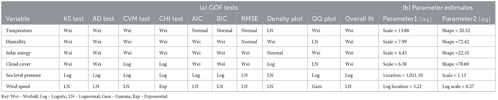
Table 5. A summary of (a) goodness-of-fit test results and (b) parameter estimates for selected weather variables.

3.4 Multivariate distributions with HAC

Figure 4 shows the HAC structures estimated from the five copula families. They reveal key insights about the hierarchical level's dependency patterns across the five copula families. The Joe, Gumbel, and Frank copulas exhibited a similar hierarchical structure as shown in Equations 27, 28:

$\begin{array}{l}\widehat{C}(u_1,u_2,u_3,u_4,u_5,u_6)=C(C(C(\text{humid},\text{cloud}),\text{windspeed}),\text{slp}),\\ C(\text{temp},\text{solar})),& (27)\end{array}$

$\begin{array}{l}\widehat{C}\left(u_1,\mathrm{...},u_6;s\right)=\left(\left(\left(\text{humid},\text{cloud}\right)\text{windspeed})\text{slp}\right)\left(\text{temp},\text{solar}\right)\right),\\ {({\theta }_1,{\theta }_2,{\theta }_3,{\theta }_4,{\theta }_5)}^T. & (28)\end{array}$

For Clayton:

$\begin{array}{l}\widehat{C}(u_1,u_2,u_3,u_4,u_5,u_6)=C(C(C(\text{humid},\text{cloud}),\text{windspeed}),\\ C(C(\text{temp},\text{solar}),\text{slp})), & (29)\end{array}$

$\begin{array}{l}\widehat{C}\left(u_1,\mathrm{...},u_6;s\right)=(\left(\left(\text{humid},\text{cloud}\right),\text{windspeed}\right),\\ \left(\left(\text{temp},\text{solar}\right),\text{slp}\right))),{({\theta }_1,{\theta }_2,{\theta }_3,{\theta }_4,{\theta }_5)}^T. & (30)\end{array}$

For AMH:

$\begin{array}{l}\widehat{C}(u_1,u_2,u_3,u_4,u_5,u_6)=C(C(C(C(\text{humid},\text{cloud}),C(\text{temp},\\ \text{ solar})),\text{slp}),\text{windspeed}),& (31)\end{array}$

$\begin{array}{l}\widehat{C}\left(u_1,\mathrm{...},u_6;s\right)=(\left(\left(\left(\text{humid},\text{cloud}\right),\left(\text{temp},\text{solar}\right)\right),\text{slp}\right)\\ \text{ windspeed})),{({\theta }_1,{\theta }_2,{\theta }_3,{\theta }_4,{\theta }_5)}^T.& (32)\end{array}$

The findings indicate the most tightly coupled pair, followed by their joint relationship with wind speed. Sea-level pressure (slp) contributed at the next level of dependency, and finally, temperature and solar energy exhibit a distinct, parallel relationship. Notably, the HAC Frank and HAC Clayton structures had independence between certain variables, diverging from the more cohesive dependence observed in Joe, Gumbel, and AMH models. This independence highlights weaker or negligible interactions between some variable pairs, making these copulas more appropriate for scenarios where dependencies are sparse or asymmetric. The temperature and solar energy in HAC Frank had the strongest pair dependence (θ₄ = 5.73, τ = 0.710) which was closely aligned with the correlation coefficient in Figure 3. Similarly, humidity and cloud cover exhibited consistently strong dependence across all HAC models, emphasizing the well-established atmospheric relationship where increased humidity levels contribute to increased cloud formation. On the other hand, very weak dependencies observed in the HAC Frank and HAC Clayton, came from sea-level pressure and wind speed, sea-level pressure and humidity, as well as humidity and wind speed, indicating minimal direct interactions between these variables.

Figure 4

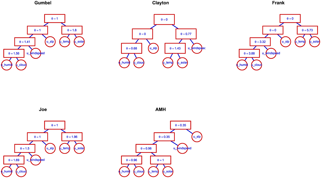
Figure 4. Hierarchical Archimedean Copula (HAC) structures and parameter estimates for climate variables across five copula families.

3.5 Model selection

The model selection criteria for the five HAC models are displayed in Table 6a. The HAC Gumbel model, highlighted in bold—had the best fit. The Clayton and AMH models showed modest fits, but the HAC Frank model came in second with comparatively good performance. The HAC Joe model, however, showed the weakest fit, as evidenced by its lower logLik. Despite the Gumbel HAC model's superior performance, further GOF tests were conducted across all five copula families to confirm the robustness of the results.

Table 6

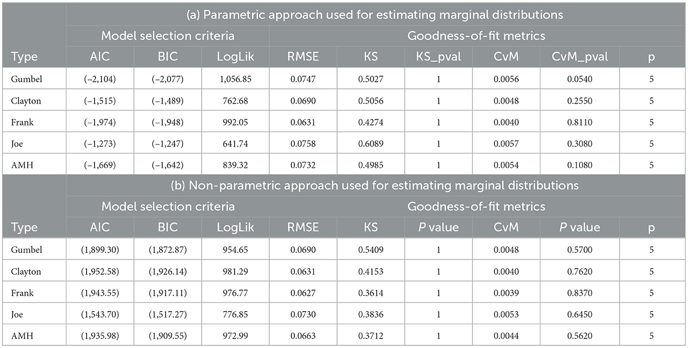
Table 6. Summary of (a) model selection criteria and (b) goodness-of-fit metrics for five HAC copula models under parametric and nonparametric marginal estimation.

3.5.1 Graphical assessment

Graphical methods and GOF tests were carried out to further determine the performance of the HAC models. Figure 5 illustrates the comparison between empirical copula values (P_e) and theoretical copula values (P_c) for five HAC models. Each plot includes the coefficient of determination R² to assess the fit of the model. The HAC Joe copula demonstrates the best fit, with the highest (R² = 0.9976), indicating its superior ability to align the theoretical and empirical values. The HAC Frank copula also had a strong performance, having the second (R² = 0.9972) after HAC Joe. The HAC Gumbel, HAC AMH and HAC Clayton copulas exhibited comparable accuracy. All models exhibit a strong linear relationship between (P_e) and (P_c), as evidenced by the proximity of the data points to the red reference line.

Figure 5

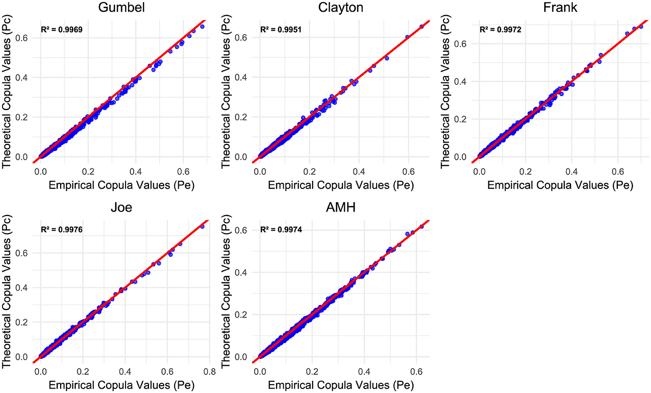
Figure 5. Comparison of empirical and theoretical copula values with goodness-of-fit metrics for five HAC models.

3.6 Goodness of fit tests

The findings of the GOF tests in Table 6a indicate that all HAC models performed well, as evidenced by their relatively small RMSE values. The HAC Frank model had the best overall fit, achieving the lowest RMSE value (0.0631) and strong CvM test performance (0.0040, p = 0.8110). This implies that the Frank copula tends to represent the data slightly better than the HAC Gumbel model, despite the latter being identified as the optimal model based on model selection criteria such as loglik, AIC, and BIC. The Gumbel HAC model exhibited a slightly higher RMSE (0.0747) but maintained strong performance in the CvM test (0.0056, p = 0.054). However, we noted that the differences between the HAC models were minimal across all GOF metrics, as was also reflected in QQ plot in Figure 5, further emphasizing the marginal variations in fit quality. Using the HAC-Frank model, we extracted parameter estimates and identified the corresponding dependency structure as shown in Equation 33:

$\begin{array}{l}{C}_{HAC-F}=C(C{\left(C(C{(\text{humid},\text{cloud})}_{\widehat{\theta }=3.88},\text{windspeed}\right)}_{\widehat{\theta }=3.32},\\ {\text{slp})}_{\widehat{\theta }=0},{C{(\text{temp},\text{solar})}_{\widehat{\theta }=5.73})}_{\widehat{\theta }=0}.& (33)\end{array}$

These were then utilized to simulate the data, which was subsequently transformed back to the original scale to enable a direct comparison with the actual observations. The purpose of this process was to evaluate the consistency between the simulated and actual data and to evaluate the effectiveness of the HAC Frank in capturing the dependencies. The summary statistics for the actual and simulated dataset are provided in Tables 4a, b respectively, while Figure 6 presents a density plot comparing their distributions. Furthermore, the scatterplot in Figure 7 illustrates the relationships among the six variables for the actual and simulated data from HAC Frank. In addition, a correlation Table 7 is also presented for assessing inter-variable dependencies.

Figure 6

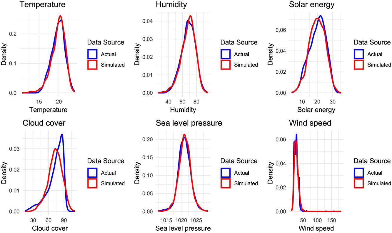
Figure 6. Density plots of temperature, humidity, solar energy, cloud cover, sea level pressure, and windspeed, shows comparison of observed data with sets of 1,461 generated random samples based on dependence parameters obtained by HAC - Frank. Blue color is observed data, and red represents simulated samples from HAC model.

Figure 7

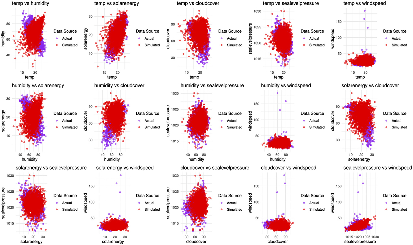
Figure 7. Pairwise scatter plots of temperature, humidity, solar energy, cloud cover, sea level pressure, windspeed, shows comparison of observed data with sets of 1,461 generated random samples based on dependence parameters obtained by HAC - Frank. Blue dots color is observed data, and red dots are simulated samples from HAC - Frank model.

Table 7

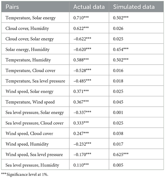
Table 7. Kendall's rank correlation coefficient of Bivariate Correlation analysis for Actual and Simulated data.

3.6.1 Comparison between HAC and vine copula

To justify the performance of the selected HAC model, a Vine copula model was employed for comparison. Vine copulas are widely used for multivariate dependency modeling due to their flexibility in capturing complex dependence structures through cascaded bivariate copulas. Based on the established marginal distributions, both R-vine and C-vine copulas were fitted, with the R-vine model emerging as the best fit according to its lower AIC and BIC values. To further validate model selection, the HAC-Frank and R-vine models were subjected to additional comparative tests, as presented in Table 8. The R-vine model outperformed the HAC model, as indicated by its lower AIC (−3, 930.25) and BIC (−3, 850.95), along with the highest logLik (1980.12). The vine copula structures also included different rotations (90°and270°) to model negative dependencies, as shown in the contour plot in Figure 8 which provides information on the strength and shape of dependencies between variable pairs. However, further GOF tests reveal a different perspective on model suitability. The ECDF comparison highlights discrepancies in model fit. HAC had a significantly lower RMSE (0.0631) compared to R-vine (0.5188), indicating a closer approximation to the actual data. HAC exhibited a much lower CVM statistic (0.0040) compared to R-vine (0.2691) and a considerably lower KS statistic (0.4274) compared to R-vine (0.9967), suggesting a better alignment with the empirical distribution. Furthermore, the WD for HAC (0.0369) was lower than that of R-vine (2.6789), implying that HAC offers a more robust estimate of the empirical distribution. In addition, HAC is computationally more efficient, requiring only 5 parameters compared to 15 in R-vine. This highlights the increased computational complexity and parameter estimation challenges in high-dimensional data when using vine copulas.

Table 8

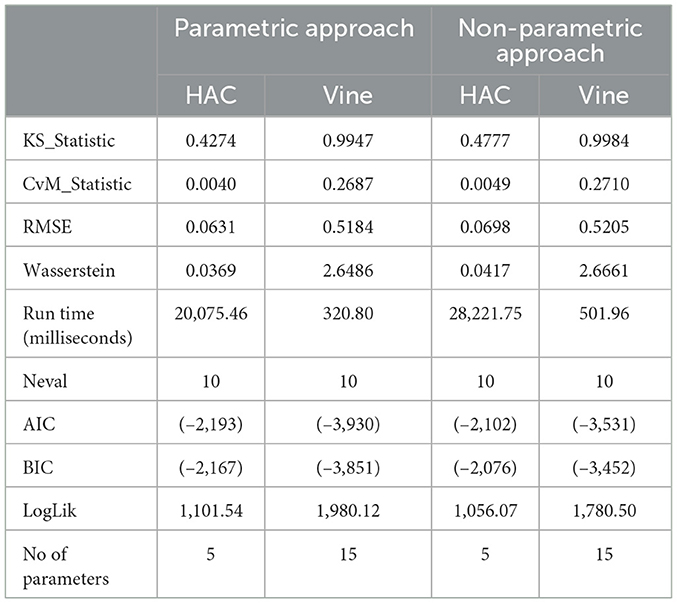
Table 8. Comparative evaluation of HAC and R-Vine Copula models using goodness-of-fit tests and computational time under parametric and non-parametric marginal estimation.

Figure 8

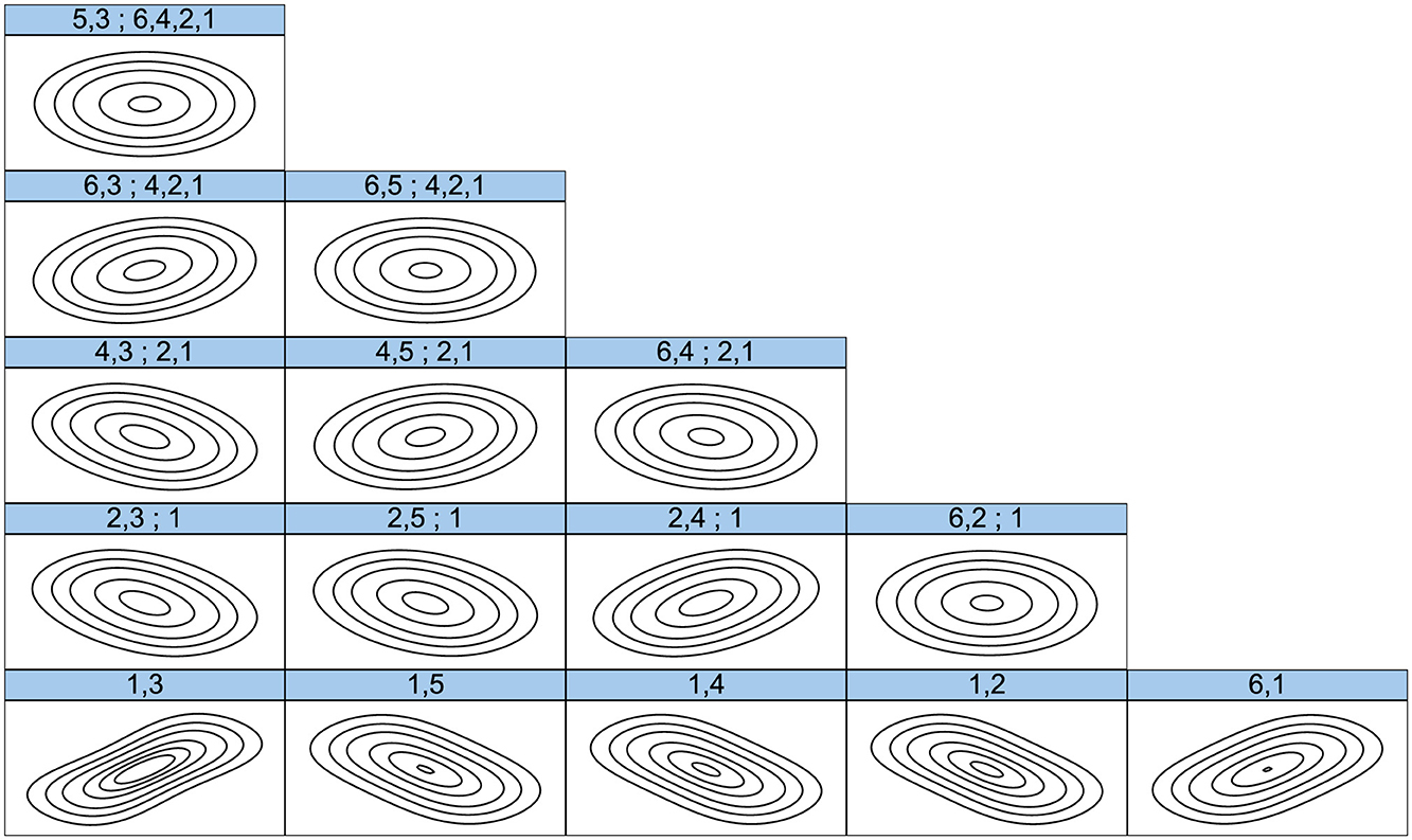
Figure 8. Contour plots of the R-vine Copula fit for temperature (1), humidity (2), solar energy (3), cloud cover (4), sea-level pressure (5), and wind speed (6). The plots illustrate the hierarchical structure of dependencies, where lower-level pairwise dependencies form the building blocks for higher-level groupings. For example, strong dependencies between temperature and solar energy (1,3) and between temperature and humidity (1,2) are combined at the second level into a new dependency structure (2,3;1). At subsequent levels, groupings such as (2,3;1) and (2,4;1) are further combined to form higher-level dependencies (4,3;2,1), eventually culminating in the final structure (5,3;6,4,2,1) that captures the overall multivariate dependence among all six climatic variables. The density and shape of the contours reflect the strength and asymmetry of the relationships: elliptical and skewed contours indicate strong or directional dependencies, while near-circular contours imply weaker interactions.

3.7 Sensitivity analysis

To assess the sensitivity of our model selection to marginal distributional assumptions and copula structure, we conducted an alternative analysis using pseudo-observations (pobs), which transform raw data into uniform margins non-parametrically. We re-fitted five HAC families—Frank, Clayton, Gumbel, Joe, and AMH—on the transformed data and re-evaluated goodness-of-fit statistics, including KS, CvM, RMSE, and AIC. A summary of the findings are provides in Table 6b. The HAC-Frank model consistently exhibited superior performance across both parametric and pobs-based settings, confirming the robustness of our model selection to marginal distribution specification.

Additionally, the R-Vine copula model was re-fitted using the pseudo-observations and compared against HAC-Frank using key fit metrics (KS, CvM, RMSE, and WD). HAC-Frank demonstrated consistently lower variability and more stable performance under nonparametric margins, whereas the R-Vine occasionally achieved better log-likelihood and information criterion values.

We further compared computational runtimes for the HAC-Frank and R-Vine copula models using parametric margins and non-parametric margins. Results in Table 8 based on 10 replicates indicate that the R-Vine model was substantially faster, completing in a mean time of 320.8 milliseconds, whereas the HAC-Frank model required approximately 20.08 seconds. This difference is attributable to the global estimation involved in HAC structures vs. the pairwise construction in Vine copulas. Despite this, the HAC-Frank model remains advantageous due to its lower parameter count (5vs.15), interpretability, and robustness to marginal assumptions, making it suitable in contexts where model transparency and parsimony are prioritized over computational speed.

4 Discussion

The primary objective of this study was to develop a multivariate joint distribution model for climatic variables in Kenya using the HAC approach. We first reviewed the correlation analysis of the six climatic variables. Our findings revealed notable disparities in the distribution of correlation strengths between the six variables. These differences showed variations in dependencies between variable in pairs, highlighting the diverse interactions within the climate system. Specifically, temperature and solar energy had a strong positive correlation, a relationship that is well supported in climatology, as higher levels of solar radiation generally led to increased temperatures due to energy absorption at the Earth's surface [64]. In addition, cloud cover and humidity depicted a strong positive correlation, which coincide with previous studies [65]. This dependence can be attributed to the fact that increased cloud cover traps moisture within the atmosphere, leading to higher humidity levels. Conversely, wind speed exhibited very weak correlations with other climatic variables such as cloud cover, humidity, and sea level pressure (r = −0.232, −0.170, and r = 0.247) respectively, indicating that wind dynamics are driven by complex atmospheric processes that cannot be fully captured using simple linear correlation measures [9]. Therefore, it is essential to employ copula-based models instead of traditional linear correlation techniques, as copulas provide flexible dependency structures that capture both linear and non-linear relationships between variables [66, 67].

An analysis of six key climatic variables revealed that temperature, humidity, solar energy, cloud cover, and wind speed were best modeled using distributions belonging to the gamma family, notably the Weibull and gamma distributions. These distributions are known to be closely nested, with the exponential and Weibull distributions being special or limiting cases of the gamma distribution [68]. This nesting supports the suitability of gamma-based models in capturing the stochastic behavior of environmental variables.

Specifically, the two-parameter Weibull distribution provided the best fit for temperature, humidity, solar energy, and cloud cover. The Weibull distribution is widely applied in climate modeling due to its capacity to represent skewed data and capture extreme values—features that are characteristic of many climatic variables. Its robustness in modeling temperature, cloud cover, and wind speed makes it a valuable tool for climate impact assessments, forecasting, and adaptive planning [35, 69].

The logistic model was found to be the appropriate model for sea-level pressure. Given that sigmoidal trends and abrupt changes in atmospheric pressure are essential for weather prediction and storm modeling, the logistic model proves to be highly valuable in climate applications [70]. Wind speed was modeled using the gamma distribution which is widely used in meteorological studies due to its ability to capture positively skewed data, a characteristic feature of wind speed observations. The gamma distribution is an important tool in studies on renewable energy and storm damage assessments, since it is effective in describing the likelihood of extreme wind events [71, 72].

Among the five fitted HAC models, the HAC-Gumbel model emerged as the best-fit model, as determined by its superior AIC, BIC & loglik value [57, 60, 67, 70, 71]. The Gumbel copula is convenient for this application because of its flexibility in accommodating upper tail dependencies. This distinguishes it from Clayton copulas, which primarily capture lower tail dependencies [19, 60, 70]. In contrast, the correlation matrix confirmed the presence of positive and negative correlations among the six climatic variables, justifying the HAC-Frank model.

The HAC Frank model offers a valuable tool for understanding how these climatic variables interact over time. We compared actual and simulated data as demonstrated in Figure 6, of the scatterplots. The findings show a replica of the real-world patterns which its applications can be expanded in the following ways: In agricultural planning, recognizing the strong connection between temperature and solar energy can significantly aid in forecasting periods of intense heat likely to cause drought stress. In drought-prone regions of Kenya, such as Marsabit and Lodwar, these findings could play a key role in developing early warning systems [73]. Government agencies like the Kenya Agricultural Research Institute (KARI) can leverage this information to advise farmers on adopting drought-tolerant crops like sorghum and millet during seasons when extended dry spells are predicted [74]. In addition, crop diversification strategies should be proposed to farmers and knowledge on planting schedules should be extended to them to ensure there is awareness of alignment with good climatic conditions. In disaster management, understanding the dependency between humidity and precipitation can provide early warnings for potential flooding events. Government agencies like the National Disaster Management Agency (NADIMA) could use these insights to prepare flood response measures in advance, especially for vulnerable regions [75, 76]. Simulating the dependence between temperature, humidity, and sea-level pressure can inform infrastructure planning and maintenance. For example, projections of extreme precipitation combined with high humidity could allow policymakers to strengthen drainage systems, reinforce vulnerable road networks, and allocate resources for maintenance ahead of seasonal peaks, particularly in urban centers such as Nairobi and Mombasa that are susceptible to climate-induced infrastructural damage [77]. In renewable energy, the relationship between solar energy and temperature is important for optimizing solar power generation. The government of Kenya through solar home developers could use model projections to schedule installations or maintenance to coincide with periods of peak solar energy availability in regions experiencing high temperatures, especially in rural homes [78].

Further assessment of the fit of the model revealed that HAC-Frank closely matched the empirical pairwise correlations, indicating its strong ability to capture underlying dependency structures in climate variables. Four key GOF metrics – KS, CVM, RMSE, and WD confirmed its superior performance highlighting a critical distinction: while HAC-Gumbel provides the best fit, HAC-Frank offers superior predictive performance, particularly in capturing complex multivariate relationships in climate variables. These findings are similar to a growing body of research that underscores the effectiveness of copula based approaches in modeling joint probability distributions of environmental variables [26, 36, 66]. However, studies that produced different results, such as Cong and Brady [16], could be attributed to variations in climatic regions, dataset characteristics, and methodological differences, reinforcing the importance of context-specific model selection.

Vine copulas outperformed the HAC model based on model selection criteria (AIC, BIC, and LogLik) [31, 35]. The strong performance of vine copulas comes from their ability to capture complex and asymmetric dependence patterns while also allowing different pairwise copulas at each hierarchical level [30, 51]. In contrast to the vine copula models, the HAC-Frank model demonstrated a better accurate fit to the dataset, according to GOF tests [35]. In addition, HAC models are effective for analyzing high-dimensional climate data, as they require fewer estimated parameters than vine copulas, thereby reducing computation complexity [35, 39]. Consequently, HAC-Frank emerges as attractive alternative for applications where computational efficiency and parsimony are key considerations.

4.1 Limitation

While this study demonstrates the usefulness of HAC models in capturing complex dependencies among climatic variables, a few limitations should be noted. First, the analysis was based on data from a single meteorological station (Nairobi Wilson Airport), with occasional supplementation from a nearby station (Jomo Kenyatta International Airport) to address missing observations. Although this approach ensured a complete dataset for analysis, it introduces some potential biases, particularly in representing localized weather extremes. Moreover, the findings from Nairobi may not fully generalize to other regions of Kenya, which experience very different climatic patterns.

Second, the proposed model adopts a homogeneous HAC structure, where all pairwise dependencies are modeled using copulas from the same Archimedean family. While this approach ensures compliance with sufficient nesting conditions, it may not capture accurately real-world climatic associations. In reality, different variable pairs may exhibit unique dependence features such as varying tail behavior or asymmetry which are better modeled using heterogeneous copula families. Hence, the homogeneous assumption may restrict the model's flexibility and reduce its ability to optimally represent the true dependence structure across all levels of the hierarchy.

5 Conclusion

This paper proposes a joint distribution framework for constructing a six-dimensional model using HACs. In this study, we demonstrated the applicability of HAC models in capturing multivariate dependencies, which are essential for climate risk assessment, agricultural sustainability, and renewable energy planning.

We illustrated a systematic approach for selecting best fitting univariate probability distributions for weather variables using multiple GOF tests and graphical assessment. By utilizing these fitted distributions, the variables were transformed to uniform margins, forming the foundation for copula -based modeling. Weibull distribution was found to be the best fit for temperature, humidity, solar energy, and cloud cover while the logistic distribution was most suitable for sea-level pressure, and the gamma distribution for wind speed.

Using RML, we estimated the structure and parameters of a HAC. Model selection and thorough GOF testing were used to identify the best HAC model for the six climatic variables. The findings confirmed that HAC models effectively capture dependencies and offer a computationally efficient alternative compared to vine copulas, making them suitable for high-dimensional climate modeling. Notably, HAC Frank emerged as the most appropriate model for the six variables.

Future research should explore the use of heterogeneous HAC models in climatic modeling, integrating spatial modeling techniques within HAC frameworks, and use of HAC models and artificial intelligence for high dimensional dependence modeling.

Data availability statement

Publicly available datasets were analyzed in this study. This data can be found here: https://www.visualcrossing.com/.

Author contributions

KO: Conceptualization, Data curation, Formal analysis, Investigation, Methodology, Resources, Software, Visualization, Writing – original draft, Writing – review & editing, Project administration, Validation. LC: Investigation, Supervision, Validation, Writing – review & editing, Conceptualization, Resources, Funding acquisition. EO: Conceptualization, Investigation, Resources, Supervision, Validation, Writing – review & editing. CO: Conceptualization, Investigation, Resources, Supervision, Validation, Writing – review & editing. BO: Resources, Supervision, Validation, Writing – review & editing, Conceptualization, Data curation, Investigation, Methodology, Project administration.

Funding

The author(s) declare that no financial support was received for the research and/or publication of this article.

Acknowledgments

The authors acknowledge with gratitude the support from Strathmore Institute of Mathematical Sciences, Strathmore University, DAAD [ST32 - PKZ: 91789473] and University of South Carolina Upstate, Division of Mathematics & Computer Science in the production of this manuscript.

Conflict of interest

The authors declare that the research was conducted in the absence of any commercial or financial relationships that could be construed as a potential conflict of interest.

Generative AI statement

The author(s) declare that no Gen AI was used in the creation of this manuscript.

Publisher's note

All claims expressed in this article are solely those of the authors and do not necessarily represent those of their affiliated organizations, or those of the publisher, the editors and the reviewers. Any product that may be evaluated in this article, or claim that may be made by its manufacturer, is not guaranteed or endorsed by the publisher.

References

1. Gebre GG, Amekawa Y, Fikadu AA, Rahut DB. Farmers use of climate change adaptation strategies and their impacts on food security in Kenya. Climate Risk Management. (2023) 40:100495. doi: 10.1016/j.crm.2023.100495

PubMed Abstract | Crossref Full Text | Google Scholar

2. IPCC. Climate Change 2022: Impacts, Adaptation and Vulnerability. Summary for Policymakers. Cambridge: New York, NY: Cambridge University Press (2022).

Google Scholar

3. IPCC. Climate Change 2007: impacts, adaptation and vulnerability: contribution of Working Group II to the fourth assessment report of the Intergovernmental Panel (2007).

Google Scholar

4. Obwocha EB, Ramisch JJ, Duguma L, Orero L. The relationship between climate change, variability, and food security: understanding the impacts and building resilient food systems in West Pokot County, Kenya. Sustainability. (2022) 14:765. doi: 10.3390/su14020765

Crossref Full Text | Google Scholar

5. Chowdhary H. Copula-Based Multivariate Hydrologic Frequency Analysis Recommended Citation (2009).

Google Scholar

6. Ribeiro AFS, Russo A, Gouveia CM, Páscoa P, Zscheischler J. Risk of crop failure due to compound dry and hot extremes estimated with nested copulas. Biogeosci Discuss. (2020) 2020:1–21. doi: 10.5194/bg-2020-116

Crossref Full Text | Google Scholar

7. Mallick H, Bhattacharyya A, Chatterjee S, Fenta HM. Joint modeling of rainfall and temperature in Bahir Dar, Ethiopia: application of copula. Front Appl Math Stat. (2023) 8:1058011. doi: 10.3389/fams.2022.1058011

Crossref Full Text | Google Scholar

8. Hao Z, Singh VP. Review of dependence modeling in hydrology and water resources. Progr Phys Geogr. (2016) 40:549–78. doi: 10.1177/0309133316632460

Crossref Full Text | Google Scholar

9. Embrechts P, McNeil A, Straumann D. Correlation pitfalls and alternatives. Risk Magaz. (1999). p. 69–71.

Google Scholar

10. Embrechts P, McNeil AJ, Straumann D. Correlation and dependence in risk management: properties and pitfalls. In: Dempster MAH, editor. Risk Management: Value at Risk and Beyond. Cambridge: Cambridge University Press (2010) 176–223. doi: 10.1017/CBO9780511615337.008

PubMed Abstract | Crossref Full Text | Google Scholar

11. Czado C, Bax K, Sahin Ö, Nagler T, Min A, Paterlini S. Vine copula based dependence modeling in sustainable finance. J Finance Data Sci. (2022) 8:309–30. doi: 10.1016/j.jfds.2022.11.003

Crossref Full Text | Google Scholar

12. Genest C, Okhrin O, Bodnar T. Copula modeling from Abe Sklar to the present day. J Multivar Anal. (2024) 201:105278. doi: 10.1016/j.jmva.2023.105278

Crossref Full Text | Google Scholar

13. Größer J, Okhrin O. Copulae: an overview and recent developments. Comput Stat. (2022) 14:e1557. doi: 10.1002/wics.1557

Crossref Full Text | Google Scholar

14. Hofert M. Correlation pitfalls with ChatGPT: would you fall for them? Risks. (2023) 11:4448522. doi: 10.2139/ssrn.4448522

Crossref Full Text | Google Scholar

15. Okhrin O, Tetereva A. The realized hierarchical Archimedean copula in risk modelling. Econometrics. (2017) 5:56. doi: 10.3390/econometrics5020026

Crossref Full Text | Google Scholar

16. Cong RG, Brady M. The interdependence between rainfall and temperature: Copula analyses. Sci World J. (2012) 2012:405675. doi: 10.1100/2012/405675

PubMed Abstract | Crossref Full Text | Google Scholar

17. Dzupire NC, Ngare P, Odongo L, A. copula based bi-variate model for temperature and rainfall processes. Sci African. (2020) 8:e00365. doi: 10.1016/j.sciaf.2020.e00365

Crossref Full Text | Google Scholar

18. Yee KC, Suhaila J, Yusof F, Mean FH. Bivariate copula in Johor rainfall data. In: AIP Conference Proceedings. vol. 1750. American Institute of Physics Inc. (2016). doi: 10.1063/1.4954624

Crossref Full Text | Google Scholar

19. Nelsen RB. An Introduction to Copulas. Cham: Springer (2006).

Google Scholar

20. Joe H. Multivariate Models and Multivariate Dependence Concepts. New York: Chapman and Hall/CRC (1997). doi: 10.1201/b13150

Crossref Full Text | Google Scholar

21. Okhrin O, Ristig A. Hierarchical Archimedean Copulae: The HAC Package (2014). Available online at: http://www.jstatsoft.org/ (accessed January 13, 2024).

Google Scholar

22. Hofert M, Scherer M. CDO pricing with nested Archimedean copulas. Quant Finan. (2011) 11:775–87. doi: 10.1080/14697680903508479

Crossref Full Text | Google Scholar

23. Okhrin O, Ristig A. Penalized estimation of hierarchical Archimedean copula. J Multivar Anal. (2024) 201:105274. doi: 10.1016/j.jmva.2023.105274

Crossref Full Text | Google Scholar

24. Favre AC, Adlouni SE, Perreault L, Thiémonge N, Bobée B. Multivariate hydrological frequency analysis using copulas. Water Resour Res. (2004) 40:2456. doi: 10.1029/2003WR002456

Crossref Full Text | Google Scholar

25. Lin-Ye J, Garcia-Leon M, Gracia V, Sanchez-Arcilla A. A multivariate statistical model of extreme events: an application to the Catalan coast. Coastal Eng. (2016) 117:138–56. doi: 10.1016/j.coastaleng.2016.08.002

Crossref Full Text | Google Scholar

26. Saad C, Adlouni SE, St-Hilaire A, Gachon P, A. nested multivariate copula approach to hydrometeorological simulations of spring floods: the case of the Richelieu River (Québec, Canada) record flood. Stochastic Environ Res Risk Assess. (2015) 29:275–94. doi: 10.1007/s00477-014-0971-7

Crossref Full Text | Google Scholar

27. Grimaldi S, Serinaldi F. Design hyetograph analysis with 3-copula function. Hydrol Sci J. (2006) 51:223–38. doi: 10.1623/hysj.51.2.223

PubMed Abstract | Crossref Full Text | Google Scholar

28. Serinaldi F, Grimaldi S. Fully Nested 3-Copula: procedure and application on hydrological data. J Hydrol Eng. (2007) 12:420. doi: 10.1061/(ASCE)1084-0699(2007)12:4(420)

Crossref Full Text | Google Scholar

29. Brechmann EC, Heiden M, Okhrin Y. A multivariate volatility vine copula model. Econometr Rev. (2018) 37:281–308. doi: 10.1080/07474938.2015.1096695

Crossref Full Text | Google Scholar

30. Joe H, Dorota K. Dependence Modeling Vine Copula Handbook. Singapore: World Scientific Publishing Company (2011). doi: 10.1142/9789814299886_0008

Crossref Full Text | Google Scholar

31. Maina SC, Mwigereri D, Weyn J, Mackey L, Ochieng M. Evaluation of dependency structure for multivariate weather predictors using copulas. ACM J Comput Sustain Soc. (2023) 1:1–23. doi: 10.1145/3616384

Crossref Full Text | Google Scholar

32. Vernieuwe H, Vandenberghe S, Baets BD, Verhoest NEC. A continuous rainfall model based on vine copulas. Hydrol Earth Syst Sci. (2015) 19:2685–99. doi: 10.5194/hess-19-2685-2015

Crossref Full Text | Google Scholar

33. Wang Z, Zhang W, Zhang Y, Liu Z. Circular-linear-linear probabilistic model based on vine copulas: An application to the joint distribution of wind direction, wind speed, and air temperature. J Wind Eng Industr Aerodyn. (2021) 215:104704. doi: 10.1016/j.jweia.2021.104704

Crossref Full Text | Google Scholar

34. Ma M, Wang X, Liu N, Song S, Wang S. Nested copula model for overall seismic vulnerability analysis of multispan bridges. Shock Vibr. (2022) 2022:3001933. doi: 10.1155/2022/3001933

Crossref Full Text | Google Scholar

35. Yang Y, Fang C, Li Y, Xu C, Liu Z. Multivariate joint distribution of five-dimensional wind and wave parameters in the sea-crossing bridge region using Hierarchical Archimedean Copulas. J Wind Eng Industr Aerodyn. (2024) 247:105684. doi: 10.1016/j.jweia.2024.105684

Crossref Full Text | Google Scholar

36. Lin-Ye J, García-León M, Grácia V, Ortego MI, Lionello P, Sánchez-Arcilla A. Multivariate statistical modelling of future marine storms. Appl Ocean Res. (2017) 65:192–205. doi: 10.1016/j.apor.2017.04.009

PubMed Abstract | Crossref Full Text | Google Scholar

37. Choroś-Tomczyk B, Härdle WK, Okhrin O. Valuation of collateralized debt obligations with hierarchical Archimedean copulae. J Empir Finance. (2013) 24:42–62. doi: 10.1016/j.jempfin.2013.08.001

Crossref Full Text | Google Scholar

38. Kubát M, Górecki J. An experimental comparison of Value at Risk estimates based on elliptical and hierarchical Archimedean copulas. In: 33rd International Conference Mathematical Methods in Economics: Conference Proceedings. Cheb (2015). p. 911.

Google Scholar

39. Okhrin O, Okhrin Y, Schmid W. On the structure and estimation of hierarchical Archimedean copulas. J Econom. (2013) 173:189–204. doi: 10.1016/j.jeconom.2012.12.001

Crossref Full Text | Google Scholar

40. VC C. Visual Crossing Weather (2025). Available online at: https://www.visualcrossing.com/ (accessed May 13, 2024).

Google Scholar

41. von Loeper F, Kirstein T, Idlbi B, Ruf H, Heilscher G, Schmidt V. Probabilistic analysis of solar power supply using d-vine copulas based on meteorological variables. In: Göttlich, S., Herty, M., Milde, A., editors. Mathematical Modeling, Simulation and Optimization for Power Engineering and Management. Mathematics in Industry. Cham: Springer (2021). doi: 10.1007/978-3-030-62732-4_3

Crossref Full Text | Google Scholar

42. Sklar A. Fonctions de répartition á n dimensions et leurs marges (Distribution functions of n dimensions and their marginals). Publications de l'Institut Statistique de l'Université de Paris (1959). p. 8.

Google Scholar

43. Okhrin O, Okhrin Y, Schmid W. Properties of hierarchical Archimedean copulas. Statist Risk Model. (2013) 30:21–54. doi: 10.1524/strm.2013.1071

Crossref Full Text | Google Scholar

44. McNeil AJ, Nešlehová J. Multivariate archimedean copulas, d-monotone functions and l 1-norm symmetric distributions. Ann Stat. (2009) 37:3059–97. doi: 10.1214/07-AOS556

PubMed Abstract | Crossref Full Text | Google Scholar

45. Kimberling CH. A probabilistic interpretation of complete monotonicity. Aequationes Mathemat. (1974) 10:152–64. doi: 10.1007/BF01832852

Crossref Full Text | Google Scholar

46. Savu C, Trede M. Hierarchies of Archimedean copulas. Quantit Finan. (2010) 10:295–304. doi: 10.1080/14697680902821733

Crossref Full Text | Google Scholar

47. Hofert M, Mächler M. Nested Archimedean copulas meet R: the nacopula package. J Stat Softw. (2011) 39:1–20. doi: 10.18637/jss.v039.i09

Crossref Full Text | Google Scholar

48. Aas K, Czado C, Frigessi A, Bakken H. Pair-copula constructions of multiple dependence. Insurance. (2009) 44:182–98. doi: 10.1016/j.insmatheco.2007.02.001

PubMed Abstract | Crossref Full Text | Google Scholar

49. Bedford T, Cooke RM. Probability density decomposition for conditionally dependent random variables modeled by vines. Ann Math Artif Intellig. (2001) 32:24568. doi: 10.1023/A:1016725902970

Crossref Full Text | Google Scholar

50. Brechmann EC, Schepsmeier U. Modeling dependence with C-and D-vine copulas: the R package CDVine. J Stat Softw. (2013) 52.

Google Scholar

51. Dißmann J, Brechmann EC, Czado C, Kurowicka D. Selecting and estimating regular vine copulae and application to financial returns. Comput Statist Data Anal. (2013) 59:52–69. doi: 10.1016/j.csda.2012.08.010

Crossref Full Text | Google Scholar

52. McNeil AJ. Sampling nested Archimedean copulas. J Stat Comput Simul. (2008) 78:567–81. doi: 10.1080/00949650701255834

Crossref Full Text | Google Scholar

53. Delignette-Muller ML, Christophe D. fitdistrplus: an R Package for Fitting Distributions. J Stat Softw. (2021) 64:1–34. doi: 10.18637/jss.v064.i04

Crossref Full Text | Google Scholar

54. Naghettini M. Fundamentals of Statistical Hydrology. Cham: Springer (2016). doi: 10.1007/978-3-319-43561-9

Crossref Full Text | Google Scholar

55. Hasan RHR. Estimating the Best-fitted probability distribution for monthly maximum temperature at the Sylhet station in Bangladesh. J Mathem Statist Stud. (2021) 2:60–7. doi: 10.32996/jmss.2021.2.2.7

Crossref Full Text | Google Scholar

56. Dodangeh E, Singh VP, Pham BT, Yin J, Yang G, Mosavi A, et al. Flood frequency analysis of interconnected rivers by copulas. Water Resour Manag. (2020) 34:3533–49. doi: 10.1007/s11269-020-02634-0

Crossref Full Text | Google Scholar

57. Fan L, Wang H, Wang C, Lai W, Zhao Y. Exploration of use of copulas in analysing the relationship between precipitation and meteorological drought in Beijing, China. Adv Meteorol. (2017) 2017:284. doi: 10.1155/2017/4650284

Crossref Full Text | Google Scholar

58. Hofert M, Kojadinovic I, Maechler M, Yan J, Maechler MM, Suggests MASS. Package ‘Copula' (2014). Available online at: http://ie.archive.ubuntu.com/disk1/disk1/cran.r-project.org/web/packages/copula/copula.pdf

Google Scholar

59. Okhrin O, Ristig A, Xu YF. Copulae in High Dimensions: An Introduction (2017). doi: 10.1007/978-3-662-54486-0_13

Crossref Full Text | Google Scholar

60. Reddy MJ, Ganguli P. Bivariate flood frequency analysis of upper godavari river flows using Archimedean copulas. Water Resour Manag. (2012) 26. doi: 10.1007/s11269-012-0124-z

Crossref Full Text | Google Scholar

61. Bernton E, Jacob PE, Gerber M, Robert CP. On parameter estimation with the Wasserstein distance. Inf Infer. (2019) 8:657–76. doi: 10.1093/imaiai/iaz003

Crossref Full Text | Google Scholar

62. Soliman M, Newlands NK, Lyubchich V, Gel YR. Financial and Statistical Methods Multivariate Copula Modeling for Improving Agricultural Risk Assessment under Climate Variability (2023). Available online at: https://www12.statcan.gc.ca/census-recensement/2011/geo/bound-limit/bound-limit-2016-eng.cfm (accessed September 13, 2024).

Google Scholar

63. Verdinelli I, Wasserman L. Hybrid Wasserstein distance and fast distribution clustering. Electron J Stat. (2019) 13:5088–119. doi: 10.1214/19-EJS1639

PubMed Abstract | Crossref Full Text | Google Scholar

64. Haigh J. Solar influences on climate. Grantham Institute for Climate Change. (2011).

Google Scholar

65. Shin JY, Kim KR, Ha JC. Seasonal forecasting of daily mean air temperatures using a coupled global climate model and machine learning algorithm for field-scale agricultural management. Agric Forest Meteorol. (2020) 281:107858. doi: 10.1016/j.agrformet.2019.107858

Crossref Full Text | Google Scholar

66. Ayantobo OO, Li Y, Song S. Copula-based trivariate drought frequency analysis approach in seven climatic sub-regions of mainland China over 1961–2013. Theor Appl Climatol. (2019) 137:2217–37. doi: 10.1007/s00704-018-2724-x

Crossref Full Text | Google Scholar

67. Genest C, Favre AC. Everything you always wanted to know about copula modeling but were afraid to ask. J Hydrol Eng. (2007) 12:347. doi: 10.1061/(ASCE)1084-0699(2007)12:4(347)

Crossref Full Text | Google Scholar

68. Wilks DS. Statistical Methods in the Atmospheric Sciences. vol 100 New York: Academic press. (2011).

Google Scholar

69. Odo FC, Offiah SU, Ugwuoke PE. Weibull distribution-based model for prediction of wind potential in Enugu, Nigeria. Adv Appl Sci Res. (2012) 3:1202–8. doi: 10.7763/AASR.2012.3.1202

Crossref Full Text | Google Scholar

70. Yavuzdoğan A. A copula approach for sea level anomaly prediction: a case study for the Black Sea. Surv Rev. (2021) 53:436–46. doi: 10.1080/00396265.2020.1816314

Crossref Full Text | Google Scholar

71. André LM. Zea Bermudez de Modelling dependence between observed and simulated wind speed data using copulas. Stochastic Environ Res Risk Assess. (2020) 34:1725–53. doi: 10.1007/s00477-020-01866-1

Crossref Full Text | Google Scholar

72. Chowdhury SN, Dhawan S. Statistical estimation for fitting wind speed distribution. In: 2016 International Conference on Energy Efficient Technologies for Sustainability, ICEETS 2016 (2016). doi: 10.1109/ICEETS.2016.7582895

Crossref Full Text | Google Scholar

73. Cooper PJ, Dimes J, Rao K, Shapiro B, Shiferaw B, Twomlow S. Coping better with current climatic variability in the rain-fed farming systems of sub-Saharan Africa: an essential first step in adapting to future climate change? Agric Ecosyst Environ. (2008) 126:24–35. doi: 10.1016/j.agee.2008.01.007

Crossref Full Text | Google Scholar

74. Herrero M, Ringler C, Steeg JVD, Thornton PK, Bryan E, Omolo A, et al. Climate Variability and Climate Change and Their Impacts on Kenya's Agricultural Sector. Nairobi, Kenya: ILRI (2010).

Google Scholar

75. Owuondo J. A review of disaster preparedness and management techniques in Kenya. Int J Res Innov Soc Sci. (2022) 6:4.

Google Scholar

76. Opilo BN, Mugalavai E. Strategies for mitigating flood risks in Western Region, Kenya. African J Empir Res. (2023) 4:1063–70. doi: 10.51867/ajernet.4.2.108

Crossref Full Text | Google Scholar

77. World Bank. Kenya Urbanization Review. World Bank (2016). Available online at: https://hdl.handle.net/10986/23753 (accessed September 13, 2024).

Google Scholar

78. Rotich IK, Chepkirui H, Musyimi PK. Renewable energy status and uptake in Kenya. Energy Strat Rev. (2024) 54:101453. doi: 10.1016/j.esr.2024.101453

Crossref Full Text | Google Scholar