Internet traffic data recovery via a low-rank spatio-temporal regularized optimization approach without d-th order T-SVD

Accurate recovery of Internet traffic data can mitigate the adverse impact of incomplete data on network task processes. In this study, we propose a low-rank recovery model for incomplete Internet traffic data with a fourth-order tensor structure, incorporating spatio-temporal regularization while avoiding the use of d-th order T-SVD. Based on d-th order tensor product, we first establish the equivalence between d-th order tensor nuclear norm and the minimum sum of the squared Frobenius norms of two factor tensors under the unitary transformation domain. This equivalence allows us to leave aside the d-th order T-SVD, significantly reducing the computational complexity of solving the problem. In addition, we integrate the alternating direction method of multipliers (ADMM) to design an efficient and stable algorithm for precise model solving. Finally, we validate the proposed approach by simulating scenarios with random and structured missing data on two real-world Internet traffic datasets. Experimental results demonstrate that our method exhibits significant advantages in data recovery performance compared to existing methods.

1 Introduction

Internet traffic data, characterized by distinct spatio-temporal attributes, are crucial for documenting information transmission volumes over specified time periods. It plays a vital role in network design and management [1–3]. However, in practice, uncontrollable factors often result in incomplete or corrupted traffic data, hindering its effective use. Therefore, accurately recovering original data from incomplete traffic data is of significant importance.

Since Zhang et al. [4] introduced the sparse regularized matrix factorization (SRMF) model for data recovery, while incorporating the unique characteristics of Internet traffic data, research in the field of Internet traffic data recovery has continued to advance. As higher-order generalizations of matrices, tensors are more effective at capturing the structural characteristics within the data. Consequently, many researchers have proposed various effective methods for Internet traffic data recovery based on different tensor decomposition techniques, such as the CANDECOMP/PARAFAC (CP) decomposition [5, 6], the tensor-train (TT) decomposition [7], and the third-order T-product factorization [8]. Given that low-rankness is a typical characteristic of incomplete data in scenarios with high levels of missing samples, low-rank modeling serves as another effective strategy beyond tensor decomposition. Candès et al. [9] were the pioneers in establishing a low-rank matrix data recovery model. To address its inherent non-convexity and NP hardness, they employed the nuclear norm of a matrix to convexly relax the model, enabling an effective solution. Unlike the definition of matrix rank, which is well-defined, the definition of tensor rank relies on specific decomposition method.

In 2014, based on the tensor singular value decomposition (T-SVD), Zhang et al. [10] proposed third-order tensor nuclear norm (TNN) and employed it to convexly relax the tubal rank of tensors, and they established a model for image restoration. On this basis, Li et al. [11] developed the SRTNN model for the recovery of Internet traffic data by incorporating spatial-temporal regularization with the nuclear norm of third-order tensors, which demonstrates significant advantages in terms of data recovery effectiveness. Meanwhile, to mitigate the computational burden associated with SVD, He et al. [12] proposed the equivalence between the so-called transformed tubal nuclear norm for a third-order tensor and the minimum of the sum of two factor tensors' squared Frobenius norms under a general invertible linear transform.

Currently, the recovery of Internet traffic data primarily relies on model construction based on third-order tensors. While these studies have achieved certain advancements, the effectiveness in restoring data with structural missingness remains limited. Addressing this challenge requires data recovery models to more thoroughly account for the intrinsic structural characteristics of the data. In the case of Internet traffic data, considering its complexity and multidimensionality, it can be organized in the form of a fourth-order tensor ($\mathcal{X}\in {ℝ}^{D\times T\times N\times N}$, where N signifies network nodes, T is the daily recording times, and D indicates the recording days) to capture the internal structural features of the data more comprehensively. Therefore, exploring a low-rank fourth-order tensor model for Internet traffic data recovery is essential.

Notably, Martin et al. [13] have extended the third order T-product to d-th order T-product, which is explained in a recursive way but for computational speed is implemented directly using the fast Fourier transform. Inspired by this, Qin et al. [14] have generalized the multiplication in the discrete Fourier transform (DFT) domain to tensor product in the domain of general invertible transforms and introduced the d-th order tensor nuclear norm. They employed the d-th order TNN to perform convex relaxation on the fourth order tensor low-rank model, establishing the HTNN method for recovering visual data. However, for solving optimization problems involving nuclear norms, the thresholding operator is often employed, which involves performing SVD on a large number of matrices during the process, significantly increasing the computational time [11, 14]. Hence, a natural question arises about how to build a low-rank recovery model for a d-th order tensor without the need for SVD computation.

In this study, by arranging the observed Internet traffic data as a tensor $\mathcal{M}\in {ℝ}^{D\times T\times N\times N}$, we enable unitary transformations on mode-3 and mode-4 to fully integrate the internal data of these modes. Meanwhile, a spatio-temporal regularization term is applied to modes-1 and-2, aiming to preserve the periodicity and similarity of the recovered data as much as possible, thereby enhancing the accuracy of data recovery. We develop a new low-rank model for the recovery of fourth-order Internet traffic data as follows:

$\begin{array}{l}\underset{{\displaystyle \mathcal{X}}}{\min }\Vert {\displaystyle \mathcal{X}}{\Vert }_{\star ,L}+\frac{{\alpha }_1}{2}\Vert H·{\text{Mat}}_1({\displaystyle \mathcal{X}}){\Vert }_F^2+\frac{{\alpha }_2}{2}\Vert K·{\text{Mat}}_2({\displaystyle \mathcal{X}}){\Vert }_F^2+\gamma \Vert {\displaystyle \mathcal{X}}{\Vert }_F^2\\ \text{s.t. }{P}_{\Omega }({\displaystyle \mathcal{X}})=P_{\Omega }(ℳ),\end{array}$

where ||·||_{⋆, L} means the tensor nuclear norm under the unitary transform L, and ${\mathrm{\text{Mat}}}_1(\mathcal{X})$ and ${\mathrm{\text{Mat}}}_2(\mathcal{X})$ are consisted by flow data of consecutive days and time points, respectively. Through the equivalence relationship between the d-th order tensor nuclear norm and the minimum sum of two factor tensors' squared Frobenius norms within the unitary transformation domain and under the d-th order T-product which is first established by us, we reformulate this model into the following version without relying on d-th order T-SVD:

$\begin{array}{l}\underset{{\displaystyle \mathcal{X}},{\displaystyle \mathcal{U}},{\displaystyle \mathcal{V}}}{\min }\frac{1}{2}(\Vert {\displaystyle \mathcal{U}}{\Vert }_F^2+\Vert {\displaystyle \mathcal{V}}{\Vert }_F^2)+\frac{\lambda }{2}\Vert {\displaystyle \mathcal{X}}-{\displaystyle \mathcal{U}}{*}_L{\displaystyle \mathcal{V}}{\Vert }_F^2+\gamma \Vert {\displaystyle \mathcal{X}}{\Vert }_F^2\\ +\frac{{\alpha }_1}{2}\Vert H·{\text{Mat}}_1({\displaystyle \mathcal{X}}){\Vert }_F^2+\frac{{\alpha }_2}{2}\Vert K·{\text{Mat}}_2({\displaystyle \mathcal{X}}){\Vert }_F^2\\ \text{ s.t. }{P}_{\Omega }({\displaystyle \mathcal{X}})=P_{\Omega }(ℳ).\end{array}$

We will give a detail explanation about these two models in Section 3.

The rest of this study is organized as follows. Some notions and preliminaries are listed in Section 2. In Section 3, we establish a low-rank Internet traffic data recovery model without d-th order tensor SVD and solve it using the alternating direction method of multipliers (ADMM), proposing a computational framework for solving the model. In Section 4, we conduct a convergence analysis of Algorithm 1, ensuring that it converges to a stationary point. Numerical experiments are presented in Section 5, where we apply the proposed method to two real-world Internet traffic datasets and simulate potential structural missingness scenarios in practice. The experimental results demonstrate that our method exhibits significant advantages, both in terms of recovery accuracy and computational efficiency. Finally, we give the conclusion of this study in Section 6.

Algorithm 1

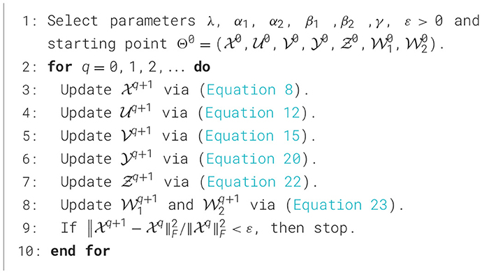
Algorithm 1. Tensor completion algorithm with d-th order tensor product decomposition and spatio-temporal regularization (SRdTPD).

2 Preliminary

In this study, the real number field and the complex number field are denoted by ℝ and ℂ, respectively. We use lowercase letters a, b, ⋯  to denote scalars, bold lowercase letters a, b, ⋯  to represent vectors, capital letters A, B, ⋯  to signify matrices, and calligraphic letters $\mathcal{A},\mathcal{B},\cdots$ to denote tensors. For any positive integer n, we define the set [n]: = {1, 2, ..., n}. For A∈ℂ^m×n, A^H denotes the conjugate transpose of A (when A is in the real number field, its transpose is A^⊤), and its nuclear norm is denoted as $\Vert A{\Vert }_{\star }={\displaystyle \sum _{i=1}^{\text{min}\{m,n\}}{\sigma }_i}(A)$, where σ_i is the i-th singular value of A. For a d-th order real tensor $\mathcal{A}=(a_{i_1{i}_2\cdots i_d})\in {ℝ}^{n_1\times n_2\times \cdots \times n_d}$, its corresponding Frobenius norm is $\Vert \mathcal{A}{\Vert }_F={({\displaystyle \sum _{i_1=1}^{n_1}\cdots }{\displaystyle \sum _{i_d=1}^{n_d}|}{a}_{i_1\cdots i_d}{|}^2)}^{1/2}$. The inner product between $\mathcal{A}\in {ℝ}^{n_1\times n_2\times \cdots \times n_d}$ and $\mathcal{B}\in {ℝ}^{n_1\times n_2\times \cdots \times n_d}$ is denoted as $\langle \mathcal{A},ℬ\rangle ={\displaystyle \sum _{i_1=1}^{n_1}\cdots }{\displaystyle \sum _{i_d=1}^{n_d}{a}_{i_1\cdots i_d}}{b}_{i_1\cdots i_d}$. Denote $\mathcal{A}(i_1,\cdots ,i_{l-1},:,i_{l+1},\cdots ,i_d)\in {ℝ}^{n_l}$ as a column vector formed by fixing all modes except for mode-l, and $\mathcal{A}(i_1,\cdots ,i_{p-1},:,i_{p+1},\cdots ,i_{q-1},:,i_{q+1},\cdots ,i_d)\in {ℝ}^{n_p\times n_q}(p<q)$ as the matrix slice along mode-p and mode-q. In particular, the matrix slice encompassing the first two modes is designated as $A^j=\mathcal{A}(:,:,i_3,\cdots ,i_d)\in {ℝ}^{n_1\times n_2}$, where j = (i_d−1)n₃⋯n_d−1+⋯+(i₄−1)n₃+i₃, i_d∈[n_d]. Denote

$\text{bdiag}({\displaystyle \mathcal{A}})=\left[\begin{array}{l}{A}^1\\ A^2\\ \ddots \\ A^J\end{array}\right]\in {ℝ}^{(n_1{n}_3{n}_4\cdots n_d)\times (n_2{n}_3{n}_4\cdots n_d)},$

where J = n₃⋯n_d. Herein, elucidate the face-wise product for d-th order tensors.

Definition 1 (Face-wise product [14]). The face-wise product $\mathcal{A}△\mathcal{B}$ of two d-th order tensors $\mathcal{A}\in {ℂ}^{n_1\times l\times n_3\times \cdots \times n_d}$ and $\mathcal{B}\in {ℂ}^{l\times n_2\times n_3\times \cdots \times n_d}$ is the element of ${ℂ}^{n_1\times n_2\times n_3\times \cdots \times n_d}$ defined according to

$\begin{array}{ll}{\displaystyle \mathcal{C}}={\displaystyle \mathcal{A}}△{\displaystyle \mathcal{B}}\iff \text{bdiag}({\displaystyle \mathcal{C}})=\text{bdiag}({\displaystyle \mathcal{A}})·\text{bdiag}({\displaystyle \mathcal{B}}).& (1)\end{array}$

For a given set of invertible transformation matrices denoted as $\{L_i\in {ℂ}^{n_i\times n_i}{\}}_{i=3}^d$, the linear transformation of a d-th order tensor $\mathcal{A}$ under L is defined as ${\mathcal{A}}_L\triangleq L(\mathcal{A})=\mathcal{A}{\times }_3{L}_3{\times }_4\cdots {\times }_d{L}_d$, where the symbol × _k represents the k-mode product of a tensor with a matrix defined in [15], and the inverse transformation of $\mathcal{A}$ under L is denoted as $L^{-1}(\mathcal{A})=\mathcal{A}{\times }_3{L}_3^{-1}{\times }_4\cdots {\times }_d{L}_d^{-1}$. Thus, when the corresponding matrices $\{L_i{\}}_{i=3}^d$ of invertible linear transforms L are unitary matrices, we can obtain

$\begin{array}{ll}||{\displaystyle \mathcal{A}}|{|}_F=||{{\displaystyle \mathcal{A}}}_L|{|}_F.& (2)\end{array}$

Next, the clear definitions for the multiplication operation and related concepts of a d-th order tensor $\mathcal{A}$ within the domain of general invertible transformations.

Definition 2 (d-th order T-product [14]). Let $\mathcal{A}\in {ℝ}^{n_1\times n_2\times \cdots \times n_d}$ and $\mathcal{B}\in {ℝ}^{n_2\times l\times n_3\times \cdots \times n_d}$. Then, the invertible linear transforms L based T-product is defined as

$\begin{array}{l}{\displaystyle \mathcal{C}}={\displaystyle \mathcal{A}}{*}_L{\displaystyle \mathcal{B}}=L^{-1}({{\displaystyle \mathcal{A}}}_L△{{\displaystyle \mathcal{B}}}_L).\end{array}$

Definition 3 (d-th order tensor conjugate transpose [14]). The invertible linear transforms L based conjugate transpose of a tensor $\mathcal{A}\in {ℂ}^{n_1\times n_2\times n_3\times \cdots \times n_d}$ is the tensor $\mathcal{B}\in {ℂ}^{n_2\times n_1\times n_3\times \cdots \times n_d}$, whose matrix slice encompassing the first two modes $ℬ(:,:,i_3,\cdots ,i_d)={({\mathcal{A}}_L(:,:,i_3,\cdots ,i_d))}^H$. We denote by ${\mathcal{A}}^H$ the conjugate transpose of a tensor $\mathcal{A}$.

Definition 4 (d-th order TNN [14]). Let $\mathcal{A}\in {ℝ}^{n_1\times \cdots \times n_d}$, the tensor nuclear norm of $\mathcal{A}$ is defined as

$\Vert {\displaystyle \mathcal{A}}{\Vert }_{\star ,L}:=\frac{1}{\rho }\Vert \text{bdiag}({{\displaystyle \mathcal{A}}}_{\text{L}}){\Vert }_{\star }\text{=}\frac{\text{1}}{\rho }{\displaystyle \sum _{{\text{i}}_{\text{3}}\text{=1}}^{{\text{n}}_{\text{3}}}\cdots }{\displaystyle \sum _{{\text{i}}_{\text{d}}\text{=1}}^{{\text{n}}_{\text{d}}}\Vert }{{\displaystyle \mathcal{A}}}_{\text{L}}(:,:,{\text{i}}_{\text{3}},\cdots ,{\text{i}}_{\text{d}}){\Vert }_{\star },$

where ρ > 0 is a positive constant determined by the invertible linear transforms L.

Remark 1. The constant ρ in the key definition and theorem arises when the corresponding matrices $\{L_i{\}}_{i=3}^d$ of invertible linear transforms L fulfill the given equation:

$\begin{array}{l}(L_d\otimes L_{d-1}\otimes \cdots \otimes L_3)·(L_d^H\otimes L_{d-1}^H\otimes \cdots \otimes L_3^H)\\ =(L_d^H\otimes L_{d-1}^H\otimes \cdots \otimes L_3^H)·(L_d\otimes L_{d-1}\otimes \cdots \otimes L_3)\\ =\rho I_{n_3{n}_4\cdots n_d},\end{array}$

where ⊗ is the Kronecker product, I is the identity matrix, and n₃n₄⋯n_d is its dimensions.

Based on Definition 4, we can draw the conclusion of the equivalence between d-th order tensor nuclear norm and the minimum of the sum of two factor tensors' squared Frobenius norms:

Theorem 1. If the corresponding matrices $\{L_i{\}}_{i=3}^d$ of invertible linear transforms L are unitary matrices, for $\mathcal{A}\in {ℝ}^{n_1\times n_2\times \cdots \times n_d}$, we have

$\Vert {\displaystyle \mathcal{A}}{\Vert }_{\star ,L}=\underset{{\displaystyle \mathcal{X}},{\displaystyle \mathcal{Y}}}{\min }\{\frac{1}{2}(\Vert {\displaystyle \mathcal{X}}{\Vert }_F^2+\Vert {\displaystyle \mathcal{Y}}{\Vert }_F^2):{\displaystyle \mathcal{A}}={\displaystyle \mathcal{X}}{*}_L{{\displaystyle \mathcal{Y}}}^H\}.$

Proof: By Definition 4, we have

$\begin{array}{l}\Vert {\displaystyle \mathcal{A}}{\Vert }_{\star ,L}=\frac{1}{\rho }{\displaystyle \sum _{i_3=1}^{n_3}\cdots }{\displaystyle \sum _{id=1}^{n_d}\Vert {{\displaystyle \mathcal{A}}}_L(:,:,i_3,i_4,\cdots ,i_d){\Vert }_{\star }}\hfill \\ =\underset{{{\displaystyle \mathcal{X}}}_L,{{\displaystyle \mathcal{Y}}}_L}{\min }\{\frac{1}{2\rho }{\displaystyle \sum _{i_3=1}^{n_3}\cdots }{\displaystyle \sum _{i_d=1}^{n_d}(\Vert {{\displaystyle \mathcal{X}}}_L(:,:,i_3,i_4,\cdots ,i_d){\Vert }_F^2}\hfill \\ +\Vert {{\displaystyle \mathcal{Y}}}_L(:,:,i_3,\cdots ,i_d){\Vert }_F^2):\hfill \\ {{\displaystyle \mathcal{X}}}_L(:,:,i_3,i_4,\cdots ,i_d)·{({{\displaystyle \mathcal{Y}}}_L(:,:,i_3,\cdots ,i_d))}^H\hfill \\ ={{\displaystyle \mathcal{A}}}_L(:,:,i_3,\cdots ,i_d)\}\hfill \\ =\underset{{\displaystyle \mathcal{X}},{\displaystyle \mathcal{Y}}}{\min }\{\frac{1}{2}(\Vert {\displaystyle \mathcal{X}}{\Vert }_F^2+\Vert {\displaystyle \mathcal{Y}}{\Vert }_F^2):{\displaystyle \mathcal{A}}={\displaystyle \mathcal{X}}{*}_L{{\displaystyle \mathcal{Y}}}^H\},\hfill \end{array}$

where the proof for the second equality can be deduced from the proofs of Lemma 5.1 and Proposition 2.1 of [16], and the reason for the third equality holding is that $\{L_i{\}}_{i=3}^d$ are unitary matrices.

3 Model and algorithm

As mentioned in the introduction, Internet traffic data consist of network traffic records measured T times daily from N origin nodes to N destination nodes. Consequently, data collected over D consecutive days can be organized as a fourth-order tensor in ℝ^D×T×N×N (i.e., n₁ = D, n₂ = T, n₃ = n₄ = N), comprehensively capturing the spatio-temporal dynamics of the network traffic.

3.1 Design of model and transformation

Based on low-rank property of observed incomplete tensor $\mathcal{M}\in {ℝ}^{n_1\times n_2\times n_3\times n_4}$, we construct a data recovery model for missing traffic data within the domain of unitary transformation (i.e., the corresponding matrices ${\left\{L_i\right\}}_{i=3}^4$ in L are unitary):

$\begin{array}{l}\underset{{\displaystyle \mathcal{X}}}{\min }\Vert {\displaystyle \mathcal{X}}{\Vert }_{\star ,L}+\frac{{\alpha }_1}{2}\Vert H·{\text{Mat}}_1({\displaystyle \mathcal{X}}){\Vert }_F^2+\frac{{\alpha }_2}{2}\Vert K·{\text{Mat}}_2({\displaystyle \mathcal{X}}){\Vert }_F^2+\gamma \Vert {\displaystyle \mathcal{X}}{\Vert }_F^2\\ \text{s.t. }{P}_{\Omega }({\displaystyle \mathcal{X}})=P_{\Omega }(ℳ),& (3)\end{array}$

where α₁, α₂, and γ are positive parameters, $\mathcal{X}\in {ℝ}^{n_1\times n_2\times n_3\times n_4}$ is the Internet traffic tensor needed to be estimated, Ω is the index set corresponding to the observed entries of $\mathcal{M}$, and P_Ω(·) is the linear operator that keeps known elements in Ω while setting the others to be zeros. Here, ${\mathrm{\text{Mat}}}_1(\mathcal{X})=\left[\mathcal{X}(:,1,1,1),\dots \mathcal{X}(:,n_2,1,1),\dots ,\mathcal{X}(:,n_2,n_3,1),\dots ,\mathcal{X}(:,n_2,n_3,n_4)\right]$ $\in {ℝ}^{n_1\times (n_2{n}_3{n}_4)}$, where adjacent rows represent flow data measurements from consecutive days. And ${\text{Mat}}_2(\mathcal{X})=[\mathcal{X}(1,:,1,1),\dots ,\mathcal{X}(n_1,:,1,1),\dots ,\mathcal{X}(n_1,:,n_3,1),\dots ,\mathcal{X}(n_1,:,n_3,n_4)]\text{}\in {ℝ}^{n_2\times (n_1{n}_3{n}_4)}$, where adjacent rows represent flow data measurements from consecutive time points. The regularization term $\gamma |\mathcal{X}|{|}_F^2$ is employed to ensure the boundedness of the sequence generated by the proposed algorithm. To better capture the periodicity of the data measured on each observation day and the similarity of the data obtained between adjacent observation time points within each day, we choose the temporal constraint matrix H = Toeplitz(0, 1, −1) of the size (n₁−1) × n₁ and K = Toeplitz(0, 1, −1) of size (n₂−1) × n₂, respectively, i.e.,

$\begin{array}{l}H={\left[\begin{array}{cccccc}1& -1& 0& \cdots & 0& 0\\ 0& 1& -1& \cdots & 0& 0\\ 0& 0& 1& \cdots & 0& 0\\ ⋮& ⋮& ⋮& \ddots & ⋮& ⋮\\ 0& 0& 0& \cdots & 1& -1\end{array}\right]}_{(n_1-1)\times n_1},\\ K={\left[\begin{array}{cccccc}1& -1& 0& \cdots & 0& 0\\ 0& 1& -1& \cdots & 0& 0\\ 0& 0& 1& \cdots & 0& 0\\ ⋮& ⋮& ⋮& \ddots & ⋮& ⋮\\ 0& 0& 0& \cdots & 1& -1\end{array}\right]}_{(n_2-1)\times n_2}.\end{array}$

It is well-known that the Equation (Model) 3 requires the so-called SVD to compute the ||·||_{⋆, L} minimization subproblem, which often takes much computing time for large-scale tensors. Therefore, with the employment of Theorem 1, we gainfully reformulate Equation (Model) 3 as the following tensor factorization version:

$\begin{array}{l}\underset{{\displaystyle \mathcal{X}},{\displaystyle \mathcal{U}},{\displaystyle \mathcal{V}}}{\min }\frac{1}{2}(\Vert {\displaystyle \mathcal{U}}{\Vert }_F^2+\Vert {\displaystyle \mathcal{V}}{\Vert }_F^2)+\frac{\lambda }{2}\Vert {\displaystyle \mathcal{X}}-{\displaystyle \mathcal{U}}{*}_L{\displaystyle \mathcal{V}}{\Vert }_F^2+\gamma \Vert {\displaystyle \mathcal{X}}{\Vert }_F^2\\ +\frac{{\alpha }_1}{2}\Vert H·{\text{Mat}}_1({\displaystyle \mathcal{X}}){\Vert }_F^2\\ +\frac{{\alpha }_2}{2}\Vert K·{\text{Mat}}_2({\displaystyle \mathcal{X}}){\Vert }_F^2\\ \text{ s.t. }{P}_{\Omega }({\displaystyle \mathcal{X}})=P_{\Omega }(ℳ),& (4)\end{array}$

where $\mathcal{U}\in {ℝ}^{n_1\times s\times n_3\times n_4},\mathcal{V}\in {ℝ}^{s\times n_2\times n_3\times n_4}$. Clearly, such an optimization model no longer requires SVD to find its solution. Therefore, we call Equation (Model) 4 a SVD-free model. Moreover, to facilitate the solution of Equation (Model) 4, we introduce auxiliary variables $\mathcal{Y},\mathcal{Z}\in {ℝ}^{n_1\times n_2\times n_3\times n_4}$. Thus, the Equation (Model) 4 is equivalently written as

$\begin{array}{l}\underset{{\displaystyle \mathcal{X}},{\displaystyle \mathcal{U}},{\displaystyle \mathcal{V}},{\displaystyle \mathcal{Y}},{\displaystyle \mathcal{Z}}}{\min }f({\displaystyle \mathcal{X}},{\displaystyle \mathcal{U}},{\displaystyle \mathcal{V}},{\displaystyle \mathcal{Y}},{\displaystyle \mathcal{Z}})=\frac{1}{2}(\Vert {\displaystyle \mathcal{U}}{\Vert }_F^2+\Vert {\displaystyle \mathcal{V}}{\Vert }_F^2)+\frac{\lambda }{2}\Vert {\displaystyle \mathcal{X}}-{\displaystyle \mathcal{U}}{*}_L{\displaystyle \mathcal{V}}{\Vert }_F^2\\ +\frac{\gamma }{2}\Vert {\displaystyle \mathcal{Y}}{\Vert }_F^2+\frac{\gamma }{2}\Vert {\displaystyle \mathcal{Z}}{\Vert }_F^2+\frac{{\alpha }_1}{2}\Vert H·{\text{Mat}}_1({\displaystyle \mathcal{Y}}){\Vert }_F^2\\ +\frac{{\alpha }_2}{2}\Vert K·{\text{Mat}}_2({\displaystyle \mathcal{Z}}){\Vert }_F^2\\ \text{ s.t. }{P}_{\Omega }({\displaystyle \mathcal{X}})=P_{\Omega }(ℳ),{\displaystyle \mathcal{Y}}={\displaystyle \mathcal{X}},{\displaystyle \mathcal{Z}}={\displaystyle \mathcal{X}}.& (5)\end{array}$

3.2 Description of algorithm

We apply the alternating direction method of multipliers (ADMM) algorithm to solve Equation (Model) 5. The augmented Lagrangian function of Equation (Model) 5 is written as follows:

$\begin{array}{l}ℒ({\displaystyle \mathcal{X}},{\displaystyle \mathcal{U}},{\displaystyle \mathcal{V}},{\displaystyle \mathcal{Y}},{\displaystyle \mathcal{Z}},{{\displaystyle \mathcal{W}}}_1,{{\displaystyle \mathcal{W}}}_2)=f({\displaystyle \mathcal{X}},{\displaystyle \mathcal{U}},{\displaystyle \mathcal{V}},{\displaystyle \mathcal{Y}},{\displaystyle \mathcal{Z}})\\ +\langle {{\displaystyle \mathcal{W}}}_1,{\displaystyle \mathcal{X}}-{\displaystyle \mathcal{Y}}\rangle +\frac{{\beta }_1}{2}\Vert {\displaystyle \mathcal{X}}-{\displaystyle \mathcal{Y}}{\Vert }_F^2+\langle {{\displaystyle \mathcal{W}}}_2,{\displaystyle \mathcal{X}}-{\displaystyle \mathcal{Z}}\rangle +\frac{{\beta }_2}{2}\Vert {\displaystyle \mathcal{X}}-{\displaystyle \mathcal{Z}}{\Vert }_F^2,& (6)\end{array}$

where ${\mathcal{W}}_1$ and ${\mathcal{W}}_2\in {ℝ}^{n_1\times n_2\times n_3\times n_4}$ are the Lagrangian multipliers, and β₁ and β₂ are positive penalty parameters. Below, given the q-th iterate ${\Theta }^q:=({\mathcal{X}}^q,{\mathcal{U}}^q,{\mathcal{V}}^q,{\mathcal{Y}}^q,{\mathcal{Z}}^q,{\mathcal{W}}_1^q,{\mathcal{W}}_2^q)$, we provide specific solutions for the updates of each variable.

▸ The $\mathcal{X}$-subproblem

We update $\mathcal{X}$ by solving the following subproblem

$\begin{array}{l}\underset{{\displaystyle \mathcal{X}}}{\min }\frac{\lambda }{2}\Vert {\displaystyle \mathcal{X}}-{{\displaystyle \mathcal{U}}}^q{*}_L{{\displaystyle \mathcal{V}}}^q{\Vert }_F^2+\langle {{\displaystyle \mathcal{W}}}_1^q,{\displaystyle \mathcal{X}}-{{\displaystyle \mathcal{Y}}}^q\rangle +\frac{{\beta }_1}{2}\Vert {\displaystyle \mathcal{X}}-{{\displaystyle \mathcal{Y}}}^q{\Vert }_F^2\\ +\langle {{\displaystyle \mathcal{W}}}_2^q,{\displaystyle \mathcal{X}}-{{\displaystyle \mathcal{Z}}}^q\rangle +\frac{{\beta }_2}{2}\Vert {\displaystyle \mathcal{X}}-{{\displaystyle \mathcal{Z}}}^q{\Vert }_F^2\\ \text{ s.t. }{P}_{\Omega }({\displaystyle \mathcal{X}})=P_{\Omega }(ℳ).& (7)\end{array}$

The solution of Equation (Model) 7 is given by

$\begin{array}{ll}{{\displaystyle \mathcal{X}}}_{ijkl}^{q+1}=\{\begin{array}{l}\frac{1}{\lambda +{\beta }_1+{\beta }_2}(\lambda {{\displaystyle \mathcal{U}}}^q{*}_L{{\displaystyle \mathcal{V}}}^q+{\beta }_1{{\displaystyle \mathcal{Y}}}^q\\ +{\beta }_2{{\displaystyle \mathcal{Z}}}^q-{{\displaystyle \mathcal{W}}}_1^q-{{\displaystyle \mathcal{W}}}_2^q{)}_{ijkl},(i,j,k,l)\cancel{\in }\Omega ,\\ {ℳ}_{ijkl}\text{ otherwise}.\end{array}& (8)\end{array}$

▸ The $\mathcal{U}$-subproblem

We update $\mathcal{U}$ by

$\begin{array}{ll}{{\displaystyle \mathcal{U}}}^{q+1}=\underset{{\displaystyle \mathcal{U}}}{\arg \min }\{\frac{1}{2}\Vert {\displaystyle \mathcal{U}}{\Vert }_F^2+\frac{\lambda }{2}\Vert {{\displaystyle \mathcal{X}}}^{q+1}-{\displaystyle \mathcal{U}}{*}_L{{\displaystyle \mathcal{V}}}^q{\Vert }_F^2\}.& (9)\end{array}$

Because the corresponding matrices ${\left\{L_i\right\}}_{i=3}^4$ in L are unitary, it holds that for j∈[n₃n₄],

$\begin{array}{ll}\begin{array}{l}\frac{1}{2}\Vert {\displaystyle \mathcal{U}}{\Vert }_F^2+\frac{\lambda }{2}\Vert {{\displaystyle \mathcal{X}}}^{q+1}-{\displaystyle \mathcal{U}}{*}_L{{\displaystyle \mathcal{V}}}^q{\Vert }_F^2\hfill \\ =\frac{1}{2}\Vert {{\displaystyle \mathcal{U}}}_L{\Vert }_F^2+\frac{\lambda }{2}\Vert {{\displaystyle \mathcal{X}}}_L^{q+1}-{{\displaystyle \mathcal{U}}}_L△{{\displaystyle \mathcal{V}}}_L^q{\Vert }_F^2\hfill \\ =\frac{1}{2}{\displaystyle \sum _{j=1}^{n_3{n}_4}(\Vert U_L^j{\Vert }_F^2+\lambda \Vert {(X_L^j)}^{q+1}-U_L^j{(V_L^j)}^q{\Vert }_F^2)}.\hfill \end{array}& (10)\end{array}$

Due to the separable structure of Equation 10 with respect to decision variables $U_L^j$ for j∈[n₃n₄], solving the Equation 9 is equivalent to solving

$\begin{array}{ll}\underset{U_L^j}{\min }\frac{1}{2}\Vert U_L^j{\Vert }_F^2+\frac{\lambda }{2}\Vert {(X_L^j)}^{q+1}-U_L^j{(V_L^j)}^q{\Vert }_F^2,j\in [n_3{n}_4],& (11)\end{array}$

whose solution is given by

$\begin{array}{l}{\left(U_L^j\right)}^{q+1}=\left(\lambda {\left(X_L^j\right)}^{q+1}{\left({\left(V_L^j\right)}^{q+1}\right)}^{\top }\right)\hfill \\ {(\lambda {\left(V_L^j\right)}^{q+1}{\left({\left(V_L^j\right)}^{q+1}\right)}^{\top }+I)}^{-1}.\hfill \end{array}$

With the help of the obtained ${(U_L^j)}^{q+1}$ for j∈[n₃n₄], we can get ${\mathcal{U}}^{q+1}$ by

$\begin{array}{ll}{{\displaystyle \mathcal{U}}}^{q+1}=L^{-1}({{\displaystyle \mathcal{U}}}_L^{q+1}).& (12)\end{array}$

▸ The $\mathcal{V}$-subproblem

We update $\mathcal{V}$ by

$\begin{array}{ll}{{\displaystyle \mathcal{V}}}^{q+1}=\underset{{\displaystyle \mathcal{V}}}{\arg \min }\{\frac{1}{2}\Vert {\displaystyle \mathcal{V}}{\Vert }_F^2+\frac{\lambda }{2}\Vert {{\displaystyle \mathcal{X}}}^{q+1}-{{\displaystyle \mathcal{U}}}^{q+1}{*}_L{\displaystyle \mathcal{V}}{\Vert }_F^2\}.& (13)\end{array}$

Similarly to $\mathcal{U}$-subproblem, solving Equation 13 is equivalent to solving the following problem:

$\begin{array}{ll}\underset{V_L^j}{\min }\frac{1}{2}\Vert V_L^j{\Vert }_F^2+\frac{\lambda }{2}\Vert {(X_L^j)}^{q+1}-{(U_L^j)}^{q+1}·V_L^j{\Vert }_F^2,& (14)\end{array}$

for every j∈[n₃n₄]. Clearly, the solution of Equation (Model) 14 is given by

$\begin{array}{l}\left({{\displaystyle V}}_L^j\right)={\left(\lambda {({({{\displaystyle U}}_L^j)}^{q+1})}^{\top }{({{\displaystyle U}}_L^j)}^{q+1}+I\right)}^{-1}\\ \left(\lambda {({({{\displaystyle U}}_L^j)}^{q+1})}^{\top }{({{\displaystyle X}}_L^j)}^{q+1}\right),\end{array}$

for every j∈[n₃n₄]. Thus, ${\mathcal{V}}^{q+1}$ can be obtained via

$\begin{array}{ll}{{\displaystyle \mathcal{V}}}^{q+1}=L^{-1}({{\displaystyle \mathcal{V}}}_L^{q+1}).& (15)\end{array}$

▸ The $\mathcal{Y}$-subproblem

We update $\mathcal{Y}$ by

$\begin{array}{l}{{\displaystyle \mathcal{Y}}}^{q+1}=\underset{{\displaystyle \mathcal{Y}}}{\arg \min }\{\frac{{\alpha }_1}{2}\Vert H·{\text{Mat}}_1({\displaystyle \mathcal{Y}}){\Vert }_F^2+\langle {{\displaystyle \mathcal{W}}}_1^q,{{\displaystyle \mathcal{X}}}^{q+1}-{\displaystyle \mathcal{Y}}\rangle \\ +\frac{{\beta }_1}{2}\Vert {{\displaystyle \mathcal{X}}}^{q+1}-{\displaystyle \mathcal{Y}}{\Vert }_F^2+\frac{\gamma }{2}\Vert {\displaystyle \mathcal{Y}}{\Vert }_F^2\},& (16)\end{array}$

which is equivalent to solving

$\begin{array}{l}\underset{{\text{Mat}}_1({\displaystyle \mathcal{Y}})}{\min }\frac{{\alpha }_1}{2}\Vert H·{\text{Mat}}_1({\displaystyle \mathcal{Y}}){\Vert }_F^2+\frac{{\beta }_1}{2}\Vert {\text{Mat}}_1({\displaystyle \mathcal{Y}})-({\text{Mat}}_1({{\displaystyle \mathcal{X}}}^{q+1})\\ +\frac{1}{{\beta }_1}{\text{Mat}}_1({{\displaystyle \mathcal{W}}}_1^q)){\Vert }_F^2+\frac{\gamma }{2}\Vert {\text{Mat}}_1({\displaystyle \mathcal{Y}}){\Vert }_F^2.& (17)\end{array}$

By the optimality condition of Equation (Model) 17, we have

$\begin{array}{l}{\alpha }_1{H}^{\top }H{\text{Mat}}_1({{\displaystyle \mathcal{Y}}}^{q+1})+{\beta }_1({\text{Mat}}_1({{\displaystyle \mathcal{Y}}}^{q+1})-({\text{Mat}}_1({{\displaystyle \mathcal{X}}}^{q+1})\\ +\frac{1}{{\beta }_1}{\text{Mat}}_1({{\displaystyle \mathcal{W}}}_1^q)))+\gamma {\text{Mat}}_1({{\displaystyle \mathcal{Y}}}^{q+1})=0,& (18)\end{array}$

which implies that the optimal solution of Equation (Model) 17 is

$\begin{array}{ll}\begin{array}{l}Ma{t}_1({{\displaystyle \mathcal{Y}}}^{q+1})=({({\alpha }_1{H}^{\top }H+({\beta }_1+\gamma )I)}^{-1}\hfill \\ ({\beta }_{1}Ma{t}_1({{\displaystyle \mathcal{X}}}^{q+1})+Ma{t}_1({{\displaystyle \mathcal{W}}}_1^q)).\hfill \end{array}& (19)\end{array}$

As a result, the optimal solution of Equation 16 is

$\begin{array}{ll}\begin{array}{l}{{\displaystyle \mathcal{Y}}}^{q+1}=IMa{t}_1({({\alpha }_1{H}^{\top }H+({\beta }_1+\gamma )I)}^{-1}\hfill \\ ({\beta }_{1}Ma{t}_1({{\displaystyle \mathcal{X}}}^{q+1})+Ma{t}_1({{\displaystyle \mathcal{W}}}_1^q))),\hfill \end{array}& (20)\end{array}$

where IMat₁(·) is the inverse of Mat₁(·).

▸ The $\mathcal{Z}$-subproblem

We update $\mathcal{Z}$ by

$\begin{array}{l}{\displaystyle \mathcal{Z}}=\underset{{\displaystyle \mathcal{Z}}}{\arg \min }\{\frac{{\alpha }_2}{2}\Vert K·{\text{Mat}}_2({\displaystyle \mathcal{Z}}){\Vert }_F^2+\langle {{\displaystyle \mathcal{W}}}_2^q,{{\displaystyle \mathcal{X}}}^{q+1}-{\displaystyle \mathcal{Z}}\rangle \\ +\frac{{\beta }_2}{2}\Vert {{\displaystyle \mathcal{X}}}^{q+1}-{\displaystyle \mathcal{Z}}{\Vert }_F^2+\frac{\gamma }{2}\Vert {\displaystyle \mathcal{Z}}{\Vert }_F^2\}.& (21)\end{array}$

Similarly to $\mathcal{Y}$-subproblem, the optimal solution of Equation 21 is

$\begin{array}{ll}\begin{array}{l}{{\displaystyle \mathcal{Z}}}^{q+1}=IMa{t}_2({({\alpha }_2{K}^{\top }K+({\beta }_2+\gamma )I)}^{-1}\hfill \\ ({\beta }_{2}Ma{t}_2({{\displaystyle \mathcal{X}}}^{q+1})+Ma{t}_2({{\displaystyle \mathcal{W}}}_2^q))),\hfill \end{array}& (22)\end{array}$

where IMat₂(·) is the inverse of Mat₂(·).

▸ The ${\mathcal{W}}_1$ and ${\mathcal{W}}_2$-subproblems

We update ${\mathcal{W}}_1$ and ${\mathcal{W}}_2$ by

$\begin{array}{ll}\begin{array}{c}{{\displaystyle \mathcal{W}}}_1^{q+1}={{\displaystyle \mathcal{W}}}_1^q+{\beta }_1({{\displaystyle \mathcal{X}}}^{q+1}-{{\displaystyle \mathcal{Y}}}^{q+1}),\\ {{\displaystyle \mathcal{W}}}_2^{q+1}={{\displaystyle \mathcal{W}}}_2^q+{\beta }_2({{\displaystyle \mathcal{X}}}^{q+1}-{{\displaystyle \mathcal{Z}}}^{q+1}).\end{array}& (23)\end{array}$

Following the above analysis, the algorithmic framework for solving Equation (Model) 5 is presented at Algorithm 1.

Remark 2. In the $\mathcal{U}$ and $\mathcal{V}$-subproblems, the inverses of two related matrices are computed directly. In the $\mathcal{Y}$ and $\mathcal{Z}$-subproblems, we first utilize the special structure of H and K to perform Cholesky decomposition on the two matrices $H^{\top }H+({\beta }_1+\gamma )I$ and $K^{\top }K+({\beta }_2+\gamma )I$, decomposing them into the product of two triangular matrices respectively, and then obtain their inverse matrices. This will significantly reduce the computational cost. In addition, considering that the inverses of the two related matrices remain constant in each round of solving the $\mathcal{Y}$ and $\mathcal{Z}$-subproblems, we only need to compute the inverses once, and in the subsequent solving of the $\mathcal{Y}$ and $\mathcal{Z}$-subproblems, we can simply call the inverse matrices directly.

4 Convergence analysis

In this section, we investigate the convergence properties of Algorithm 1. Although the convergence of ADMM algorithm for solving the general multi-block optimization cannot be guaranteed [17], we can still use the special structure of the Equation (Model) 5 to obtain the convergence of Algorithm 1, whose proofs are similar to the proofs in Section 3.2 of [18]. We first present the Karush-Kuhn-Tucker (KKT) conditions for Equation (Model) 5:

$\begin{array}{ll}{\nabla }_{{{\displaystyle \mathcal{X}}}_{{\Omega }^c}}f({\displaystyle \mathcal{X}},{\displaystyle \mathcal{U}},{\displaystyle \mathcal{V}},{\displaystyle \mathcal{Y}},{\displaystyle \mathcal{Z}})+{{\displaystyle \mathcal{W}}}_{1{\Omega }^c}+{{\displaystyle \mathcal{W}}}_{2{\Omega }^c}={{\displaystyle \mathcal{O}}}_{{\Omega }^c},& (24)\end{array}$

$\begin{array}{ll}{\nabla }_{{\displaystyle \mathcal{U}}}f({\displaystyle \mathcal{X}},{\displaystyle \mathcal{U}},{\displaystyle \mathcal{V}},{\displaystyle \mathcal{Y}},{\displaystyle \mathcal{Z}})={\displaystyle \mathcal{O}},& (25)\end{array}$

$\begin{array}{ll}{\nabla }_{{\displaystyle \mathcal{V}}}f({\displaystyle \mathcal{X}},{\displaystyle \mathcal{U}},{\displaystyle \mathcal{V}},{\displaystyle \mathcal{Y}},{\displaystyle \mathcal{Z}})={\displaystyle \mathcal{O}},& (26)\end{array}$

$\begin{array}{ll}{\nabla }_{{\displaystyle \mathcal{Y}}}f({\displaystyle \mathcal{X}},{\displaystyle \mathcal{U}},{\displaystyle \mathcal{V}},{\displaystyle \mathcal{Y}},{\displaystyle \mathcal{Z}})-{{\displaystyle \mathcal{W}}}_1={\displaystyle \mathcal{O}},& (27)\end{array}$

$\begin{array}{ll}{\nabla }_{{\displaystyle \mathcal{Z}}}f({\displaystyle \mathcal{X}},{\displaystyle \mathcal{U}},{\displaystyle \mathcal{V}},{\displaystyle \mathcal{Y}},{\displaystyle \mathcal{Z}})-{{\displaystyle \mathcal{W}}}_2={\displaystyle \mathcal{O}},& (28)\end{array}$

$\begin{array}{ll}{P}_{\Omega }({\displaystyle \mathcal{X}})=P_{\Omega }(M),& (29)\end{array}$

$\begin{array}{ll}{\displaystyle \mathcal{Y}}={\displaystyle \mathcal{X}},& (30)\end{array}$

$\begin{array}{ll}{\displaystyle \mathcal{Z}}={\displaystyle \mathcal{X}},& (31)\end{array}$

where Ω^c represents the complement of the set Ω. Moreover, we call $({\mathcal{X}}^{•},{\mathcal{U}}^{•},{\mathcal{V}}^{•},{\mathcal{Y}}^{•},{\mathcal{Z}}^{•},{\mathcal{W}}_1^{•},{\mathcal{W}}_2^{•})$ satisfying (Equations 24–31) a stationary point of Equation (Model) 5, where ${\mathcal{W}}_1^{•}$ and ${\mathcal{W}}_2^{•}$ are Lagrange multipliers associated with the constraints ${\mathcal{Y}}^{•}={\mathcal{X}}^{•}$ and ${\mathcal{Z}}^{•}={\mathcal{X}}^{•}$, respectively. For any integer q≥0, denote ${\Theta }^q=({\mathcal{X}}^q,{\mathcal{U}}^q,{\mathcal{V}}^q,{\mathcal{Y}}^q,{\mathcal{Z}}^q,{\mathcal{W}}_1^q,{\mathcal{W}}_2^q)$.

Proposition 1. Let $\{{\Theta }^q=({\mathcal{X}}^q,{\mathcal{U}}^q,{\mathcal{V}}^q,{\mathcal{Y}}^q,{\mathcal{Z}}^q,{\mathcal{W}}_1^q,{\mathcal{W}}_2^q){\}}_{q=0}^{\infty }$ be the sequence generated by Algorithm 1. Then, we have

$\begin{array}{l}ℒ({{\displaystyle \mathcal{X}}}^{q+1},{{\displaystyle \mathcal{U}}}^q,{{\displaystyle \mathcal{V}}}^q,{{\displaystyle \mathcal{Y}}}^q,{{\displaystyle \mathcal{Z}}}^q,{{\displaystyle \mathcal{W}}}_1^q,{{\displaystyle \mathcal{W}}}_2^q)+\frac{\lambda +{\beta }_1+{\beta }_2}{2}\Vert {{\displaystyle \mathcal{X}}}^{q+1}-{{\displaystyle \mathcal{X}}}^q{\Vert }_F^2\\ \le ℒ({{\displaystyle \mathcal{X}}}^q,{{\displaystyle \mathcal{U}}}^q,{{\displaystyle \mathcal{V}}}^q,{{\displaystyle \mathcal{Y}}}^q,{{\displaystyle \mathcal{Z}}}^q,{{\displaystyle \mathcal{W}}}_1^q,{{\displaystyle \mathcal{W}}}_2^q).& (32)\end{array}$

Proof: We consider three cases: (a) Ω = ∅, (b) ∅⊊Ω⊊[n₁] × [n₂] × [n₃] × [n₄], and (c) Ω = [n₁] × [n₂] × [n₃] × [n₄]. In case (a), the $\mathcal{X}$-subproblem Equation (Model) 7 becomes an unconstrained optimization problem, which is equivalent to ${\text{min}}_{\mathcal{X}}{f}_1(\mathcal{X})$, where

$\begin{array}{ll}{f}_1({\displaystyle \mathcal{X}})=\frac{\lambda }{2}\Vert {\displaystyle \mathcal{X}}-{{\displaystyle \mathcal{C}}}^q{\Vert }_F^2+\frac{{\beta }_1}{2}\Vert {\displaystyle \mathcal{X}}-{{\displaystyle D}}^q{\Vert }_F^2+\frac{{\beta }_2}{2}\Vert {\displaystyle \mathcal{X}}-{ℰ}^q{\Vert }_F^2& (33)\end{array}$

with ${\mathcal{C}}^q={\mathcal{U}}^q{*}_L{\mathcal{V}}^q$, ${\mathcal{D}}^q={\mathcal{Y}}^q-(1/{\beta }_1){\mathcal{W}}_1^q$ and ${\mathcal{E}}^q={\mathcal{Z}}^q-(1/{\beta }_2){\mathcal{W}}_2^q$. It is obvious that f₁ is strongly convex with modulus at least λ+β₁+β₂. Consequently, by Theorem 5.24 in [19], it holds that

$\begin{array}{ll}{f}_1({{\displaystyle \mathcal{X}}}^{\prime })\ge f_1({\displaystyle \mathcal{X}})+\langle \nabla f_1({\displaystyle \mathcal{X}}),{{\displaystyle \mathcal{X}}}^{\prime }-{\displaystyle \mathcal{X}}\rangle +\frac{\lambda +{\beta }_1+{\beta }_2}{2}\Vert {{\displaystyle \mathcal{X}}}^{\prime }-{\displaystyle \mathcal{X}}{\Vert }_F^2& (34)\end{array}$

for any $\mathcal{X},{\mathcal{X}}^{\prime }\in {ℝ}^{n_1\times n_2\times n_3\times n_4}$. Since ${\mathcal{X}}^{q+1}$ is the optimal solution of ${\text{min}}_{\mathcal{X}}{f}_1(\mathcal{X})$, which means $\nabla f_1({\mathcal{X}}^{q+1})=\mathcal{O}$, from Equation (Inequality) 34, it holds that

$\begin{array}{ll}{f}_1({{\displaystyle \mathcal{X}}}^q)\ge f_1({{\displaystyle \mathcal{X}}}^{q+1})+\frac{\lambda +{\beta }_1+{\beta }_2}{2}||{{\displaystyle \mathcal{X}}}^q-{{\displaystyle \mathcal{X}}}^{q+1}{||}_F^2,& (35)\end{array}$

which implies, together with the definition of $\mathcal{L}$, that Equation (Inequality) 32 holds.

In the case ∅⊊Ω⊊[n₁] × [n₂] × [n₃] × [n₄], the simple equality constraints in Equation (Model) 7 can be eliminated by substituting them into its objective function, and the corresponding $\mathcal{X}$-subproblem is converted into an unconstrained optimization problem, whose objective function is similar to the structure of f₁, but $\mathcal{X}$, ${\mathcal{C}}^q$, ${\mathcal{D}}^q$, and ${\mathcal{E}}^q$ are replaced by ${\mathcal{X}}_{{\Omega }^c}$, ${\mathcal{C}}_{{\Omega }^c}^q$, ${\mathcal{D}}_{{\Omega }^c}^q$, and ${\mathcal{E}}_{{\Omega }^c}^q$, respectively. Noticing ${\mathcal{X}}_{\Omega }^{q+1}={\mathcal{M}}_{\Omega }$, similar to the proof for the case (a), we know that Equation (Inequality) 32 still holds. In the case (c), since ${\mathcal{X}}^{q+1}={\mathcal{X}}^q=\mathcal{M}$, the inequality [Equation (Inequality) 32] is obvious. We complete the proof.

Proposition 2. Let $\{{\Theta }^q{\}}_{q=0}^{\infty }$ be the sequence generated by Algorithm 1. Then we have

$\begin{array}{l}ℒ({{\displaystyle \mathcal{X}}}^{q+1},{{\displaystyle \mathcal{U}}}^{q+1},{{\displaystyle \mathcal{V}}}^q,{{\displaystyle \mathcal{Y}}}^q,{{\displaystyle \mathcal{Z}}}^q,{{\displaystyle \mathcal{W}}}_1^q,{{\displaystyle \mathcal{W}}}_2^q)+\frac{1}{2}\Vert {{\displaystyle \mathcal{U}}}^{q+1}-{{\displaystyle \mathcal{U}}}^q{\Vert }_F^2\\ \le ℒ({{\displaystyle \mathcal{X}}}^{q+1},{{\displaystyle \mathcal{U}}}^q,{{\displaystyle \mathcal{V}}}^q,{{\displaystyle \mathcal{Y}}}^q,{{\displaystyle \mathcal{Z}}}^q,{{\displaystyle \mathcal{W}}}_1^q,{{\displaystyle \mathcal{W}}}_2^q)& (36)\end{array}$

and

$\begin{array}{l}ℒ({{\displaystyle \mathcal{X}}}^{q+1},{{\displaystyle \mathcal{U}}}^{q+1},{{\displaystyle \mathcal{V}}}^{q+1},{{\displaystyle \mathcal{Y}}}^q,{{\displaystyle \mathcal{Z}}}^q,{{\displaystyle \mathcal{W}}}_1^q,{{\displaystyle \mathcal{W}}}_2^q)+\frac{1}{2}\Vert {{\displaystyle \mathcal{V}}}^{q+1}-{{\displaystyle \mathcal{V}}}^q{\Vert }_F^2\\ \le ℒ({{\displaystyle \mathcal{X}}}^{q+1},{{\displaystyle \mathcal{U}}}^{q+1},{{\displaystyle \mathcal{V}}}^q,{{\displaystyle \mathcal{Y}}}^q,{{\displaystyle \mathcal{Z}}}^q,{{\displaystyle \mathcal{W}}}_1^q,{{\displaystyle \mathcal{W}}}_2^q).& (37)\end{array}$

Proof: For every j∈[n₃n₄] and integer q≥0, we define the function $f_{jq}:{ℂ}^{n_1\times s}\to ℝ$ by

$f_{jq}(U_L^j)=\frac{1}{2}\Vert U_L^j{\Vert }_F^2+\frac{\lambda }{2}\Vert {(X_L^j)}^{q+1}-U_L^j{(V_L^j)}^q{\Vert }_F^2.$

It is obvious that f_jq is strongly convex with modulus at least 1. Similar to the proof for (a) of Proposition 1, we have

$f_{jq}({(U_L^j)}^{q+1})+\frac{1}{2}\Vert {(U_L^j)}^{q+1}-{(U_L^j)}^q{\Vert }_F^2\le f_{jq}({(U_L^j)}^q),$

which implies, together with the fact (Equation 2), that

$\begin{array}{l}\frac{1}{2}\Vert {{\displaystyle \mathcal{U}}}^{q+1}{\Vert }_F^2+\frac{\lambda }{2}\Vert {{\displaystyle \mathcal{X}}}^{q+1}-{{\displaystyle \mathcal{U}}}^{q+1}{*}_L{{\displaystyle \mathcal{V}}}^q{\Vert }_F^2+\frac{1}{2}\Vert {{\displaystyle \mathcal{U}}}^{q+1}-{{\displaystyle \mathcal{U}}}^q{\Vert }_F^2\\ \le \frac{1}{2}\Vert {{\displaystyle \mathcal{U}}}^q{\Vert }_F^2+\frac{\lambda }{2}\Vert {{\displaystyle \mathcal{X}}}^{q+1}-{{\displaystyle \mathcal{U}}}^q{*}_L{{\displaystyle \mathcal{V}}}^q{\Vert }_F^2\end{array}$

Moreover, by the definition of $\mathcal{L}$, we know that the first inequality in Equation (Inequality) 36 holds. The inequality [Equation (Inequality) 37] can be proved similarly.

Employing a proof analogous to that of Proposition 1, we can derive the following proposition.

Proposition 3. Let $\{{\Theta }^q{\}}_{q=0}^{\infty }$ be the sequence generated by Algorithm 1. Then, we have

$\begin{array}{l}ℒ({{\displaystyle \mathcal{X}}}^{q+1},{{\displaystyle \mathcal{U}}}^{q+1},{{\displaystyle \mathcal{V}}}^{q+1},{{\displaystyle \mathcal{Y}}}^{q+1},{{\displaystyle \mathcal{Z}}}^q,{{\displaystyle \mathcal{W}}}_1^q,{{\displaystyle \mathcal{W}}}_2^q)+\frac{{\beta }_1+\gamma }{2}\Vert {{\displaystyle \mathcal{Y}}}^{q+1}-{{\displaystyle \mathcal{Y}}}^q{\Vert }_F^2\\ \le ℒ({{\displaystyle \mathcal{X}}}^{q+1},{{\displaystyle \mathcal{U}}}^{q+1},{{\displaystyle \mathcal{V}}}^{q+1},{{\displaystyle \mathcal{Y}}}^q,{{\displaystyle \mathcal{Z}}}^q,{{\displaystyle \mathcal{W}}}_1^q,{{\displaystyle \mathcal{W}}}_2^q),& (38)\end{array}$

and

$\begin{array}{l}ℒ({{\displaystyle \mathcal{X}}}^{q+1},{{\displaystyle \mathcal{U}}}^{q+1},{{\displaystyle \mathcal{V}}}^{q+1},{{\displaystyle \mathcal{Y}}}^{q+1},{{\displaystyle \mathcal{Z}}}^{q+1},{{\displaystyle \mathcal{W}}}_1^q,{{\displaystyle \mathcal{W}}}_2^q)\\ +\frac{{\beta }_2+\gamma }{2}\Vert {{\displaystyle \mathcal{Z}}}^{q+1}-{{\displaystyle \mathcal{Z}}}^q{\Vert }_F^2\\ \le ℒ({{\displaystyle \mathcal{X}}}^{q+1},{{\displaystyle \mathcal{U}}}^{q+1},{{\displaystyle \mathcal{V}}}^{q+1},{{\displaystyle \mathcal{Y}}}^{q+1},{{\displaystyle \mathcal{Z}}}^q,{{\displaystyle \mathcal{W}}}_1^q,{{\displaystyle \mathcal{W}}}_2^q).& (39)\end{array}$

Denote

$\begin{array}{l}{\xi }_1={\beta }_1({\beta }_1+\gamma )-2{({\alpha }_1{\sigma }_1(H^{\top }H)+\gamma )}^2\text{ and }\hfill \\ {\xi }_2={\beta }_2({\beta }_2+\gamma )-2{({\alpha }_2{\sigma }_1(K^{\top }K)+\gamma )}^2).\hfill \end{array}$

From Propositions 1, 2, and 3, we have the following theorem, which characterizes the sufficient decrease property and boundedness of the sequence $\{{\Theta }^q{\}}_{q=0}^{\infty }$.

Theorem 2. Let $\{{\Theta }^q{\}}_{q=0}^{\infty }$ be the sequence generated by Algorithm 1. If ξ₁>0 and ξ₂>0, then the sequence $\{{\Theta }^q{\}}_{q=0}^{\infty }$ satisfies

$\begin{array}{ll}ℒ({\Theta }^{q+1})+\mu \Vert {\Lambda }^{q+1}-{\Lambda }^q{\Vert }_F^2\le ℒ({\Theta }^q),& (40)\end{array}$

where ${\Lambda }^q=({\mathcal{X}}^q,{\mathcal{U}}^q,{\mathcal{V}}^q,{\mathcal{Y}}^q,{\mathcal{Z}}^q)$ and μ = (1/2)min1, λ+β₁+β₂, ξ₁/β₁, ξ₂/β₂. Furthermore, if ${\eta }_1:={\beta }_1\gamma -{({\alpha }_1{\sigma }_1(H^{\top }H)+\gamma )}^2>0$ and ${\eta }_2:={\beta }_2\gamma -{({\alpha }_2{\sigma }_1(K^{\top }K)+\gamma )}^2>0$, then the sequence ${\left\{{\Theta }^q\right\}}_{q=0}^{\infty }$ is bounded.

Proof: From Equations 6, 23, we have

$\begin{array}{l}ℒ({\Theta }^{q+1})=ℒ({{\displaystyle \mathcal{X}}}^{q+1},{{\displaystyle \mathcal{U}}}^{q+1},{{\displaystyle \mathcal{V}}}^{q+1},{{\displaystyle \mathcal{Y}}}^{q+1},{{\displaystyle \mathcal{Z}}}^{q+1},{{\displaystyle \mathcal{W}}}_1^q,{{\displaystyle \mathcal{W}}}_2^q)\\ +\frac{1}{{\beta }_1}\Vert {{\displaystyle \mathcal{W}}}_1^{q+1}-{{\displaystyle \mathcal{W}}}_1^q{\Vert }_F^2+\frac{1}{{\beta }_2}\Vert {{\displaystyle \mathcal{W}}}_2^{q+1}-{{\displaystyle \mathcal{W}}}_2^q{\Vert }_F^2.& (41)\end{array}$

Moreover, from Equations (Inequalities) 32, 36, 38, we have

$\begin{array}{l}ℒ({{\displaystyle \mathcal{X}}}^{q+1},{{\displaystyle \mathcal{U}}}^{q+1},{{\displaystyle \mathcal{V}}}^{q+1},{{\displaystyle \mathcal{Y}}}^{q+1},{{\displaystyle \mathcal{Z}}}^{q+1},{{\displaystyle \mathcal{W}}}_1^q,{{\displaystyle \mathcal{W}}}_2^q)\\ +\frac{\lambda +{\beta }_1+{\beta }_2}{2}\Vert {{\displaystyle \mathcal{X}}}^{q+1}-{{\displaystyle \mathcal{X}}}^q{\Vert }_F^2\\ +\frac{1}{2}\Vert {{\displaystyle \mathcal{U}}}^{q+1}-{{\displaystyle \mathcal{U}}}^q{\Vert }_F^2+\frac{1}{2}\Vert {{\displaystyle \mathcal{V}}}^{q+1}-{{\displaystyle \mathcal{V}}}^q{\Vert }_F^2\\ +\frac{{\beta }_1+\gamma }{2}\Vert {{\displaystyle \mathcal{Y}}}^{q+1}-{{\displaystyle \mathcal{Y}}}^q{\Vert }_F^2+\frac{{\beta }_2+\gamma }{2}\Vert {{\displaystyle \mathcal{Z}}}^{q+1}-{{\displaystyle \mathcal{Z}}}^q{\Vert }_F^2\\ \le ℒ({\Theta }^q).& (42)\end{array}$

Consequently, by Equation 41 and Equation (Inequality) 42, it holds that

$\begin{array}{l}ℒ({\Theta }^{q+1})+\frac{\lambda +{\beta }_1+{\beta }_2}{2}\Vert {{\displaystyle \mathcal{X}}}^{q+1}-{{\displaystyle \mathcal{X}}}^q{\Vert }_F^2+\frac{1}{2}\Vert {{\displaystyle \mathcal{U}}}^{q+1}-{{\displaystyle \mathcal{U}}}^q{\Vert }_F^2\\ +\frac{1}{2}\Vert {{\displaystyle \mathcal{V}}}^{q+1}-{{\displaystyle \mathcal{V}}}^q{\Vert }_F^2+\frac{{\beta }_1+\gamma }{2}\Vert {{\displaystyle \mathcal{Y}}}^{q+1}-{{\displaystyle \mathcal{Y}}}^q{\Vert }_F^2\\ +\frac{{\beta }_2+\gamma }{2}\Vert {{\displaystyle \mathcal{Z}}}^{q+1}-{{\displaystyle \mathcal{Z}}}^q{\Vert }_F^2\\ \le ℒ({\Theta }^q)+\frac{1}{{\beta }_1}\Vert {{\displaystyle \mathcal{W}}}_1^{q+1}-{{\displaystyle \mathcal{W}}}_1^q{\Vert }_F^2+\frac{1}{{\beta }_2}\Vert {{\displaystyle \mathcal{W}}}_2^{q+1}-{{\displaystyle \mathcal{W}}}_2^q{\Vert }_F^2.& (43)\end{array}$

On the other hand, it holds that

$\begin{array}{ll}{\text{Mat}}_1({{\displaystyle \mathcal{W}}}_1^{q+1})=({\alpha }_1{H}^{\top }H+\gamma I){\text{Mat}}_1({{\displaystyle \mathcal{Y}}}^{q+1})& (44)\end{array}$

for every q≥0. Consequently, by Equation 44, we have

$\begin{array}{ll}\begin{array}{l}\Vert {{\displaystyle \mathcal{W}}}_1^{q+1}-{{\displaystyle \mathcal{W}}}_1^q{\Vert }_F^2=\Vert Ma{t}_1({{\displaystyle \mathcal{W}}}_1^{q+1})-Ma{t}_1({{\displaystyle \mathcal{W}}}_1^q){\Vert }_F^2\hfill \\ \le {({\alpha }_1{\sigma }_1(H^{\top }H)+\gamma )}^2\Vert Ma{t}_1({{\displaystyle \mathcal{Y}}}^{q+1})\hfill \\ -Ma{t}_1({{\displaystyle \mathcal{Y}}}^q){\Vert }_F^2\hfill \\ ={({\alpha }_1{\sigma }_1(H^{\top }H)+\gamma )}^2\Vert {{\displaystyle \mathcal{Y}}}^{q+1}-{{\displaystyle \mathcal{Y}}}^q{\Vert }_F^2.\hfill \end{array}& (45)\end{array}$

Similarly, we have

$\begin{array}{ll}{\text{Mat}}_1({{\displaystyle \mathcal{W}}}_2^{q+1})=({\alpha }_2{K}^{\top }K+\gamma I){\text{Mat}}_2({{\displaystyle \mathcal{Z}}}^{q+1})& (46)\end{array}$

for every q≥0, which implies

$\begin{array}{ll}\Vert {{\displaystyle \mathcal{W}}}_2^{q+1}-{{\displaystyle \mathcal{W}}}_2^q{\Vert }_F^2\le {({\alpha }_2{\sigma }_1(K^{\top }K)+\gamma )}^2\Vert {{\displaystyle \mathcal{Z}}}^{q+1}-{{\displaystyle \mathcal{Z}}}^q{\Vert }_F^2.& (47)\end{array}$

Combining Equations (Inequalities) 43 with 45 and 47, we obtain

$\begin{array}{l}ℒ({\Theta }^{q+1})+\frac{\lambda +{\beta }_1+{\beta }_2}{2}\Vert {{\displaystyle \mathcal{X}}}^{q+1}-{{\displaystyle \mathcal{X}}}^q{\Vert }_F^2+\frac{1}{2}\Vert {{\displaystyle \mathcal{U}}}^{q+1}-{{\displaystyle \mathcal{U}}}^q{\Vert }_F^2\\ +\frac{1}{2}\Vert {{\displaystyle \mathcal{V}}}^{q+1}-{{\displaystyle \mathcal{V}}}^q{\Vert }_F^2+\frac{{\xi }_1}{2{\beta }_1}\Vert {{\displaystyle \mathcal{Y}}}^{q+1}-{{\displaystyle \mathcal{Y}}}^q{\Vert }_F^2+\frac{{\xi }_2}{2{\beta }_2}\Vert {{\displaystyle \mathcal{Z}}}^{q+1}-{{\displaystyle \mathcal{Z}}}^q{\Vert }_F^2\\ \le ℒ({\Theta }^q).& (48)\end{array}$

Finally, by the definition of μ, we know that Equation (Inequality) 40 holds.

Now, we prove the boundedness of $\{{\Theta }^q{\}}_{q=0}^{\infty }$. Because $||{\mathcal{W}}_1^q|{|}_F^2\le {({\alpha }_1{\sigma }_1(H^{\top }H)+\gamma )}^2||{\mathcal{Y}}^q|{|}_F^2$ and $||{\mathcal{W}}_2^q|{|}_F^2\le {({\alpha }_2{\sigma }_1(K^{\top }K)+\gamma )}^2||{\mathcal{Z}}^q|{|}_F^2$ for any q≥0, by Equation 6, we can obtain

$\begin{array}{l}ℒ({\Theta }^q)\ge f(X^q,{{\displaystyle \mathcal{U}}}^q,{{\displaystyle \mathcal{V}}}^q,{{\displaystyle \mathcal{Y}}}^q,{{\displaystyle \mathcal{Z}}}^q)+\frac{{\beta }_1}{2}\Vert {{\displaystyle \mathcal{X}}}^q-{{\displaystyle \mathcal{Y}}}^q+\frac{1}{{\beta }_1}{{\displaystyle \mathcal{W}}}_1^q{\Vert }_F^2\\ -\frac{{({\alpha }_1{\sigma }_1(H^{\top }H)+\gamma )}^2}{2{\beta }_1}\Vert {{\displaystyle \mathcal{Y}}}^q{\Vert }_F^2\\ +\frac{{\beta }_2}{2}\Vert {{\displaystyle \mathcal{X}}}^q-{{\displaystyle \mathcal{Z}}}^q+\frac{1}{{\beta }_2}{{\displaystyle \mathcal{W}}}_2^q{\Vert }_F^2-\frac{{({\alpha }_2{\sigma }_1(K^{\top }K)+\gamma )}^2}{2{\beta }_2}\Vert {{\displaystyle \mathcal{Z}}}^q{\Vert }_F^2& (49)\end{array}$

for every q≥0. According to Equation (Inequality) 40, for any q≥0, it is clear that

$\begin{array}{ll}ℒ({\Theta }^q)+\mu {\displaystyle \sum _{s=0}^{q-1}\Vert }{\Lambda }^{s+1}-{\Lambda }^s{\Vert }_F^2\le ℒ({\Theta }^0),& (50)\end{array}$

Therefore, by the definition of f, as well as Equation 6 and Equation (Inequalities) 49, 50, it holds that for any q≥0,

$\begin{array}{l}\Vert {{\displaystyle \mathcal{U}}}^q{\Vert }_F^2\le 2ℒ({\Theta }^0),\Vert {{\displaystyle \mathcal{V}}}^q{\Vert }_F^2\le 2ℒ({\Theta }^0),{\eta }_1\Vert {{\displaystyle \mathcal{Y}}}^q{\Vert }_F^2\le 2{\beta }_1ℒ({\Theta }^0)\text{ and}\\ {\eta }_2\Vert {{\displaystyle \mathcal{Z}}}^q{\Vert }_F^2\le 2{\beta }_2ℒ({\Theta }^0).& (51)\end{array}$

Since η₁>0, η₂>0, we know that $\{({\mathcal{U}}^q,{\mathcal{V}}^q,{\mathcal{Y}}^q,{\mathcal{Z}}^q){\}}_{q=0}^{\infty }$ is bounded, which implies the boundedness of $\{({\mathcal{W}}_1^q,{\mathcal{W}}_2^q){\}}_{q=0}^{\infty }$ from Equations 44, 46. In addition, since ${\beta }_1||{\mathcal{X}}^q-{\mathcal{Y}}^q+(1/{\beta }_1){\mathcal{W}}_1^q|{|}_F^2\le 2\mathcal{L}({\Theta }^0)$ for any q≥0, which from Equation (Inequality) 49, it follows that $\{{\mathcal{X}}^q{\}}_{q=0}^{\infty }$ is also bounded. Based on the comprehensive analysis presented above, we have completed the proof.

Remark 3. Given the predefined dimensions of matrices H and K, the singular values of H^⊤H and K^⊤K can be computed. Consequently, we only need to select appropriate parameters that satisfy the hypotheses stated in Theorem 2.

Theorem 3. For the sequence $\{{\Theta }^q{\}}_{q=0}^{\infty }$ generated by Algorithm 1. If the parameters satisfy the conditions in Theorem 2, then any cluster point Θ^∞ of $\{{\Theta }^q{\}}_{q=0}^{\infty }$ is a stationary point of Equation (Model) 5.

Proof: According to Theorem 2, the sequence ${\left\{{\Theta }^q\right\}}_{q=0}^{\infty }$ is bounded. Let ${\left\{{\Theta }^{q_i}\right\}}_{i=0}^{\infty }$ be a convergent subsequence such that $\underset{i\to \infty }{lim}{\Theta }^{q_i}={\Theta }^{\infty }:=({\mathcal{X}}^{\infty },{\mathcal{U}}^{\infty },{\mathcal{V}}^{\infty },{\mathcal{Y}}^{\infty },{\mathcal{Z}}^{\infty },{\mathcal{W}}_1^{\infty },{\mathcal{W}}_2^{\infty })$. First, from Equation (Inequality) 50, we have

$\begin{array}{ll}\mu {\displaystyle \sum _{q=0}^{q_i}\Vert }{\Lambda }^{q+1}-{\Lambda }^q{\Vert }_F^2\le ℒ({\Theta }^0)-ℒ({\Theta }^{q_i}).& (52)\end{array}$

Taking the limit of both sides of the Equation 52 as i approaches ∞, it holds that

$\begin{array}{ll}\mu {\displaystyle \sum _{q=0}^{\infty }\Vert }{\Lambda }^{q+1}-{\Lambda }^q{\Vert }_F^2\le ℒ({\Theta }^0)-ℒ({\Theta }^{\infty })\le \infty ,& (53)\end{array}$

which means $\underset{q\to \infty }{lim}||{\Lambda }^{q+1}-{\Lambda }^q|{|}_F=0$. Moreover, from the optimality conditions of $\mathcal{X}$-subproblem to $\mathcal{Z}$-subproblem, as well as the update of ${\mathcal{W}}_1$ and ${\mathcal{W}}_2$, it is easy to see that

$\begin{array}{ll}\{\begin{array}{l}{\nabla }_{{{\displaystyle \mathcal{X}}}_{{\Omega }^c}}f({{\displaystyle \mathcal{X}}}^{q_i+1},{{\displaystyle \mathcal{U}}}^{q_i},{{\displaystyle \mathcal{V}}}^{q_i},{{\displaystyle \mathcal{Y}}}^{q_i},{{\displaystyle \mathcal{Z}}}^{q_i})+{({{\displaystyle \mathcal{W}}}_1^{q_i})}_{{\Omega }^c}+{\beta }_1{({{\displaystyle \mathcal{X}}}^{q_i+1}-{{\displaystyle \mathcal{Y}}}^{q_i})}_{{\Omega }^c}\hfill \\ +{({{\displaystyle \mathcal{W}}}_2^{q_i})}_{{\Omega }^c}+{\beta }_1{({{\displaystyle \mathcal{X}}}^{q_i+1}-{{\displaystyle \mathcal{Z}}}^{q_i})}_{{\Omega }^c}={{\displaystyle \mathcal{O}}}_{{\Omega }^c},\hfill \\ {({{\displaystyle \mathcal{X}}}^{q_i+1})}_{\Omega }={(ℳ)}_{\Omega },\hfill \\ {\nabla }_{{\displaystyle \mathcal{U}}}f({{\displaystyle \mathcal{X}}}^{q_i+1},{{\displaystyle \mathcal{U}}}^{q_i+1},{{\displaystyle \mathcal{V}}}^{q_i},{{\displaystyle \mathcal{Y}}}^{q_i},{{\displaystyle \mathcal{Z}}}^{q_i})={\displaystyle \mathcal{O}},\hfill \\ {\nabla }_{{\displaystyle \mathcal{V}}}f({{\displaystyle \mathcal{X}}}^{q_i+1},{{\displaystyle \mathcal{U}}}^{q_i+1},{{\displaystyle \mathcal{V}}}^{q_i+1},{{\displaystyle \mathcal{Y}}}^{q_i},{{\displaystyle \mathcal{Z}}}^{q_i})={\displaystyle \mathcal{O}},\hfill \\ {\nabla }_{{\displaystyle \mathcal{Y}}}f({{\displaystyle \mathcal{X}}}^{q_i+1},{{\displaystyle \mathcal{U}}}^{q_i+1},{{\displaystyle \mathcal{V}}}^{q_i+1},{{\displaystyle \mathcal{Y}}}^{q_i+1},{{\displaystyle \mathcal{Z}}}^{q_i})-{{\displaystyle \mathcal{W}}}_1^{q_i}={\displaystyle \mathcal{O}},\hfill \\ {\nabla }_{{\displaystyle \mathcal{Z}}}f({{\displaystyle \mathcal{X}}}^{q_i+1},{{\displaystyle \mathcal{U}}}^{q_i+1},{{\displaystyle \mathcal{V}}}^{q_i+1},{{\displaystyle \mathcal{Y}}}^{q_i+1},{{\displaystyle \mathcal{Z}}}^{q_i+1})-{{\displaystyle \mathcal{W}}}_2^{q_i}={\displaystyle \mathcal{O}},\hfill \\ {{\displaystyle \mathcal{W}}}_1^{q_i+1}={{\displaystyle \mathcal{W}}}_1^{q_i}+{\beta }_1({{\displaystyle \mathcal{X}}}^{q_i+1}-{{\displaystyle \mathcal{Y}}}^{q_i+1}),\hfill \\ {{\displaystyle \mathcal{W}}}_2^{q_i+1}={{\displaystyle \mathcal{W}}}_2^{q_i}+{\beta }_1({{\displaystyle \mathcal{X}}}^{q_i+1}-{{\displaystyle \mathcal{Z}}}^{q_i+1}).\hfill \end{array}& (54)\end{array}$

Since $\underset{i\to \infty }{lim}||{\Lambda }^{q_i+1}-{\Lambda }^{q_i}|{|}_F=0$ and $\underset{i\to \infty }{lim}{\Theta }^{q_i}={\Theta }^{\infty }$, it holds that ${\lim }_{i\to \infty }\left|\right|{\mathcal{W}}_1^{q_i+1}-{\mathcal{W}}_1^{q_i}|{|}_F=0$ from Equation (Inequality) 45. Similarly, we have $\underset{i\to \infty }{lim}||{\mathcal{W}}_2^{q_i+1}-{\mathcal{W}}_2^{q_i}|{|}_F=0$ from Equation (Inequality) 47. Consequently, by letting i → ∞ in Equation 54, we know that Θ^∞ is a stationary point of Equation (Model) 5. We complete the proof.

5 Numerical experiments

In this section, we apply our approach (SRdTPD) to two authentic Internet traffic datasets: the GÉANT dataset [20], which logs Internet traffic data from 23 original nodes to 23 destination nodes every 15 min, and the Abilene¹ dataset, which records Internet traffic data from 11 original nodes to 11 destination nodes every 5 min. For both datasets, we select data spanning a period of 7 days. The sizes of these two datasets, arranged in fourth-order tensor format, are 7 × 96 × 23 × 23 and 7 × 288 × 11 × 11, respectively. For each experiment situation, we reconstruct the Internet traffic data 5 times, and all experimental results presented are the average of five repetitions. As demonstrated by the recovery test results for synthetic experiments and many real-world applications [14], algorithms with the discrete Fourier transform not only exhibit similar recovery accuracy but also incur lower computational costs, compared to methods utilizing the discrete cosine transform or random orthogonal transform. It is well-known that the most basic Fast Fourier Transform (FFT) has a computational complexity of O(NlogN) [21]. Using this result, it is not difficult to see that the computational complexity of SRdTPD using FFT is O(n₁+n₂)n₁n₂+slog(n₃n₄)n₃n₄, which is significantly lower than that of methods using other transforms. Considering the potential computational cost advantage of SRdTPD equipped with FFT when processing large-scale data, we choose normalized discrete Fourier transform as L₃ and L₄ in L, i.e.,

$\begin{array}{l}{L}_3=L_4=\frac{1}{\sqrt{N}}\left[\begin{array}{ccccc}1& 1& 1& \cdots & 1\\ 1& w& w^2& \cdots & w^{N-1}\\ 1& w^2& w^4& \cdots & w^{2(N-1)}\\ ⋮& ⋮& ⋮& \ddots & ⋮\\ 1& w^{N-1}& w^{2(N-1)}& \cdots & w^{{(N-1)}^2}\end{array}\right]\end{array}$

with the $w=e^{-i\frac{2\pi }{N}}$. All the experiments are performed on a notebook computer (13th Gen Intel(R) Core(TM) i9-13900HX CPU @2.20 GHz with 24G memory) running a 64-bit Windows Operating System. The code of SRdTPD is released at https://github.com/Duan-Yuxuan/Traffic-data-recovery/tree/master.

To verify the performance of SRdTPD, we compare it with five existing approaches designed for data recovery, the first of which is a matrix completion method, and the remaining four are tensor completion methods:

• SRMF, which is a low-rank matrix completion with a spatio-temporal regularization [4];

• CPWOPT, which is a tensor CP factorization completion approach [22];

• T2C, which is a tensor filling approach that decomposes third-order tensors into three third-order low-rank tensors in a balanced manner [23];

• SRTNN, which is a tensor-based approach with spatio-temporal regularization terms [11];

• BGCP, which is a Bayesian Gaussian CP tensor decomposition approach [24].

We use the Normalized Mean Absolute Error (NMAE) to measure the quality of the recovered data by models and algorithms, where the NMAE is defined as follows

$\begin{array}{l}\text{NMAE}=\frac{{\displaystyle \sum _{(i,j,k,l)\notin \Omega }}|{({{\displaystyle \mathcal{X}}}_{\text{true}})}_{ijkl}-{({{\displaystyle \mathcal{X}}}_{\text{rec}})}_{ijkl}|}{{\displaystyle \sum _{(i,j,k,l)\notin \Omega }}|{({{\displaystyle \mathcal{X}}}_{\text{true}})}_{ijkl}|},\end{array}$

where ${\mathcal{X}}_{\mathrm{\text{true}}}$ and ${\mathcal{X}}_{\mathrm{\text{rec}}}$ are original data and recovered data, respectively. Clearly, lower NMAE value means better quality of the recovered data. We first consider the recovery effectiveness of various approaches for missing data with data sample rates ranging from 10% to 90%. Under random missingness in the GÉANT dataset, we set α₁ = 0.1, α₂ = 200, β₁ = 0.01, α₂ = 10, λ = 0.001, γ = 0.01, while for the Abilene dataset, we choose α₁ = β₂ = 0.01, α₂ = 10, β₁ = λ = γ = 0.001. Figure 1 presents the NMAE values for missing data recovery using various methods at different sampling rates. It can be visually observed that SRdTPD outperforms other methods in terms of data recovery effectiveness, particularly as the missing data rate increases, where the superiority of our method's recovery performance becomes increasingly apparent.

Figure 1

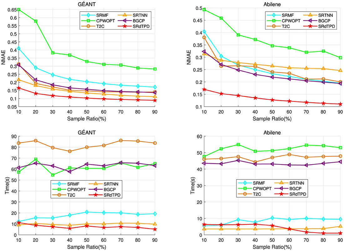
Figure 1. Numerical comparison on NMAE and computing time (seconds) with respect to different random sample ratios.

In addition to the recovery of data missing at random, we next consider the following four types of structural missingness scenarios, which are given in [4], thereby demonstrating that our method fully exploits the structural information within the data.

• xxTimeRandLoss This scenario simulates the phenomenon of structured data absence at specific time points influenced by certain factors, such as the utilization of unreliable data transmission equipment. Specifically, these data are missing at these specific time points in a certain random proportion. In our simulation, we randomly select xx% of the matrix slices along the last two modes of the Internet traffic tensor $\mathcal{X}$ of size n₁×n₂×n₃×n₄, and subsequently, we further randomly delete q% of its elements in each selected matrix.

• xxElemRandLoss This scenario simulates the structured absence of data for specific OD (Origination-Destination) nodes under the influence of certain factors, such as the use of unreliable data transmission equipment. In this context, OD node data are missing in a certain random proportion. To simulate this phenomenon, we randomly select xx% of the matrix slices along the first two modes of the Internet traffic tensor $\mathcal{X}$ of size n₁×n₂×n₃×n₄ and further randomly delete q% of the elements in each selected matrix.

• xxElemSyncLoss This scenario simulates the structured data missingness for specific OD nodes due to a uniform underlying cause, resulting in temporally synchronized missingness among these OD nodes. To emulate this condition, we randomly select xx% of the slices from the Internet traffic tensor $\mathcal{X}$ of size n₁×n₂×n₃×n₄, which are matrix representations expanded along its first two modes. Subsequently, for each selected matrix, we randomly choose a common set of time indices (q%) and delete the corresponding elements at these indices.

• RowRandLoss With flow level measurements, data are collected by a router. If a router is unable to collect data for a period of time, all data collected during those specific time points will be missing. To simulate this scenario, we randomly select p% of the time points within a day and delete all data recorded at those time points across a 7-day period.

Under these scenarios of structural missingness, with β₁ = γ = 0.01, the parameters for the first two structural missingness cases are identical within the same dataset (GÉANT: α₁ = 0.1, α₂ = 200, β₂ = 10, λ = 0.001; Abilene: α₁ = 0.1, α₂ = 2, β₂ = 1, λ = 0.001), while the parameters for the last two structural missingness cases are consistent within the same dataset (GÉANT: α₁ = 0.01, α₂ = 2, β₂ = 1, λ = 0.01; Abilene: α₁ = 0.01, α₂ = 1, β₂ = 0.1, λ = 0.01). Among these four types of structured missingness scenarios, we simulate the first three by considering the following 12 specific missingness cases: Missing Id 1-4: Set xx = 25 and, correspondingly, set q = 30, 50, 70, and 90, respectively; Missing Id 5-8: Set xx = 50 and, correspondingly, set q = 30, 50, 70, and 90, respectively; Missing Id 9-12: Set xx = 75 and, correspondingly, set q = 30, 50, 70, and 90, respectively. For the fourth type of structured missingness, we specifically select p = 15, 30, 45, 50, and 75.

The recovery performance and computational time of different methods under distinct structural missingness scenarios are comprehensively presented in Figures 2–4, Table 1. Experimental results demonstrate that the proposed SRdTPD approach achieves substantial improvements in handling structurally missing data. Regarding recovery accuracy, SRdTPD demonstrates superior performance compared to listed methods, attaining competitive results across all test cases. In terms of computational efficiency, SRdTPD maintains favorable time — while a moderate increase in computational time is observed under extreme missingness conditions (attributable to iterative process requirements), the runtime remains within practical thresholds for real-world applications. These findings collectively suggest that SRdTPD effectively balances recovery accuracy and computational demands, providing a robust solution for structural missing data recovery tasks.

Figure 2

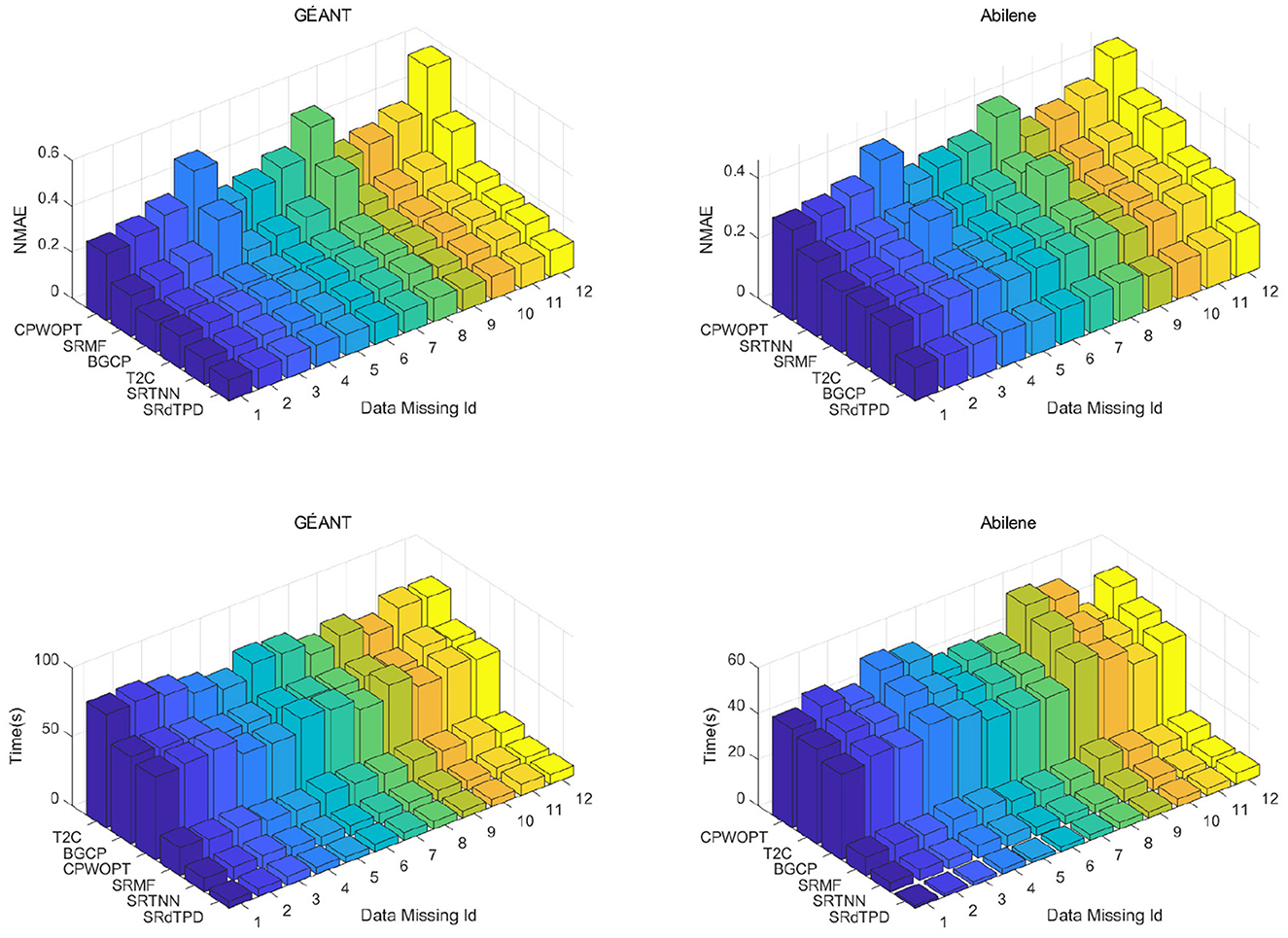
Figure 2. Numerical comparison on NMAE and computing time (seconds) with respect to different cases of xxTimeRandLoss.

Figure 3

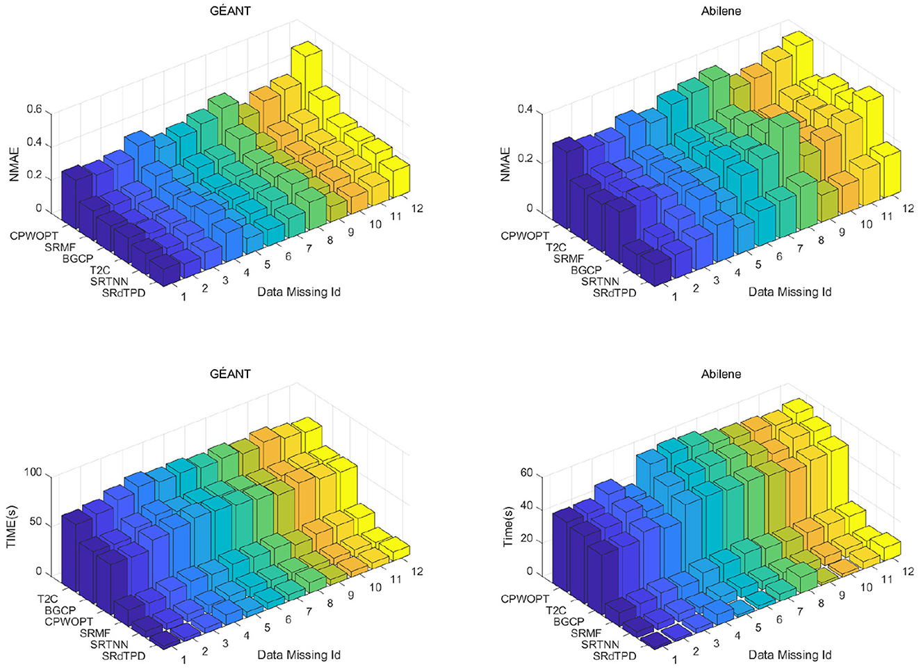
Figure 3. Numerical comparison on NMAE and computing time (seconds) with respect to different cases of xxElemRandLoss.

Figure 4

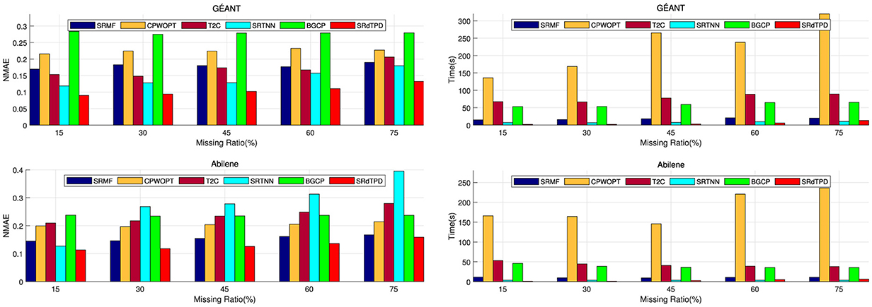
Figure 4. Numerical comparison on NMAE and computing time (seconds) with respect to diverse missing ratio of RowRandLoss.

Table 1

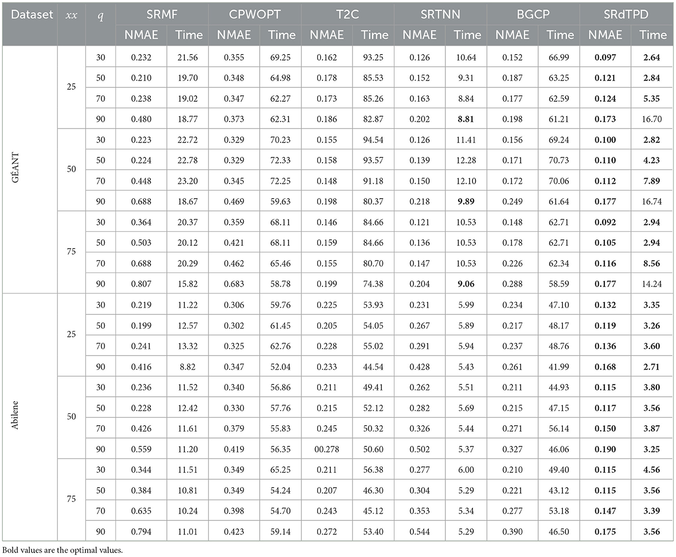
Table 1. Results on NMAE and computing time (seconds) with respect to diverse cases of xxElemSyncLoss.

6 Conclusion

This study establishes an equivalence relationship between the d-th order tensor nuclear norm (TNN) in the unitary transformation domain and the squared sum of the Frobenius norms of its two factorization factors. Based on this relationship, we constructed a novel low-rank recovery method for Internet traffic data that effectively incorporates the spatio-temporal characteristics of traffic data while significantly reducing computational time. Auxiliary variables are introduced into the model solution process, which is then solved using the ADMM. Numerical experiments demonstrate that the proposed method exhibits significant advantages in the recovery of Internet traffic data, particularly in cases of structural missingness.

Data availability statement

The raw data supporting the conclusions of this article will be made available by the authors, without undue reservation.

Author contributions

YD: Investigation, Methodology, Writing – original draft. CL: Validation, Writing – review & editing. JL: Validation, Writing – review & editing. XY: Validation, Writing – review & editing.

Funding

The author(s) declare that financial support was received for the research and/or publication of this article. CL's work was supported in part by National Natural Science Foundation of China (No. 11971138). JL's work was supported by the Science and Technology Research Program of Chongqing Municipal Education Commission (Grant No. KJZD-K202200506), by Chongqing Talent Program Lump-sum Project (No. cstc2022ycjh-bgzxm0040), and by the Foundation of Chongqing Normal University (22XLB005, ncamc2022-msxm02). XY's work was supported by the Major Program of National Natural Science Foundation of China (Nos. 11991020, 11991024).

Conflict of interest

The authors declare that the research was conducted in the absence of any commercial or financial relationships that could be construed as a potential conflict of interest.

Generative AI statement

The author(s) declare that no Gen AI was used in the creation of this manuscript.

Publisher's note

All claims expressed in this article are solely those of the authors and do not necessarily represent those of their affiliated organizations, or those of the publisher, the editors and the reviewers. Any product that may be evaluated in this article, or claim that may be made by its manufacturer, is not guaranteed or endorsed by the publisher.

Footnotes

1. ^http://abilene.internet2.edu/observatory/data-collections.html

References

1. Roughan M, Thorup M, Zhang Y. Traffic engineering with estimated traffic matrices. In: Proceedings of the 3rd ACM SIGCOMM Conference on Internet Measurement. Miami Beach, FL: Association for Computing Machinery (2003). p. 248–258.

Google Scholar

2. Cahn RS Wide area network design: concepts and tools for optimization. IEEE Commun Mag. (2000) 38:28–30. doi: 10.1109/MCOM.2000.867843

Crossref Full Text | Google Scholar

3. Zhang Y, Ge Z, Greenberg A, Roughan M. Network anomography. In: Proceedings of the 5th ACM SIGCOMM conference on Internet Measurement. Berkeley, CA: USENIX Association (2005). p. 30.

Google Scholar

4. Zhang Y, Roughan M, Willinger W, Qiu L. Spatio-temporal compressive sensing and internet traffic matrices. In: Proceedings of the ACM SIGCOMM 2009 Conference on Data Communication. Barcelona: Association for Computing Machinery (2009). p. 267–278.

Google Scholar

5. Carroll JD, Chang JJ. Analysis of individual differences in multidimensional scaling via an N-way generalization of “Eckart-Young” decomposition. Psychometrika. (1970) 35:283–319. doi: 10.1007/BF02310791

Crossref Full Text | Google Scholar

6. Harshman RA, et al. Foundations of the PARAFAC procedure: Models and conditions for an “explanatory” multi-modal factor analysis. In: UCLA Work Papers Phonetics. Ann Arbor; Los Angeles, CA: University Microfilms (1970). p. 84.

Google Scholar

7. Oseledets IV. Tensor-train decomposition. SIAM J Sci Comput. (2011) 33:2295–317. doi: 10.1137/090752286

Crossref Full Text | Google Scholar

8. Kilmer ME, Martin CD. Factorization strategies for third-order tensors. Linear Algebra Appl. (2011) 435:641–58. doi: 10.1016/j.laa.2010.09.020

Crossref Full Text | Google Scholar

9. Candès E, Recht B. Exact matrix completion via convex optimization. Found Comput Math. (2009) 9:717–72. doi: 10.1007/s10208-009-9045-5

Crossref Full Text | Google Scholar

10. Zhang Z, Ely G, Aeron S, Hao N, Kilmer M. Novel methods for multilinear data completion and de-noising based on tensor-SVD. In: 2014 IEEE Conference on Computer Vision and Pattern Recognition. Columbus, OH: IEEE (2014). p. 3842–3849.

Google Scholar

11. Li C, Chen Y, Li D. Internet traffic tensor completion with tensor nuclear norm. Comput Optim Appl. (2024) 87:1033–57. doi: 10.1007/s10589-023-00545-5

Crossref Full Text | Google Scholar

12. He H, Ling C, Xie W. Tensor completion via a generalized transformed tensor T-product decomposition without t-SVD. J Sci Comput. (2022) 93:47. doi: 10.1007/s10915-022-02006-3

Crossref Full Text | Google Scholar

13. Martin CD, Shafer R, LaRue B. An order-p tensor factorization with applications in imaging. SIAM J Sci Comput. (2013) 35:A474–90. doi: 10.1137/110841229

Crossref Full Text | Google Scholar

14. Qin W, Wang H, Zhang F, Wang J, Luo X, Huang T. Low-rank high-order tensor completion with applications in visual data. IEEE Trans Image Process. (2022) 31:2433–48. doi: 10.1109/TIP.2022.3155949

PubMed Abstract | Crossref Full Text | Google Scholar

15. Kolda TG, Bader BW. Tensor decompositions and applications. SIAM Rev. (2009) 51:455–500. doi: 10.1137/07070111X

Crossref Full Text | Google Scholar

16. Recht B, Fazel M, Parrilo PA. Guaranteed minimum-rank solutions of linear matrix equations via nuclear norm minimization. SIAM Rev. (2010) 52:471–501. doi: 10.1137/070697835

Crossref Full Text | Google Scholar

17. Chen C, He B, Ye Y, Yuan X. The direct extension of ADMM for multi-block convex minimization problems is not necessarily convergent. Math Program. (2016) 155:57–79. doi: 10.1007/s10107-014-0826-5

Crossref Full Text | Google Scholar

18. Popa J, Lou Y, Minkoff SE. Low-rank tensor data reconstruction and denoising via ADMM: algorithm and convergence analysis. J Sci Comput. (2023) 97:49. doi: 10.1007/s10915-023-02364-6

Crossref Full Text | Google Scholar

19. Beck A. First-Order Methods in Optimization. Philadelphia: SIAM. (2017). doi: 10.1137/1.9781611974997

Crossref Full Text | Google Scholar

20. Uhlig S, Quoitin B, Lepropre J, Balon S. Providing public intradomain traffic matrices to the research community. ACM SIGCOMM Comput Commun Rev. (2006) 36:83–6. doi: 10.1145/1111322.1111341

Crossref Full Text | Google Scholar

21. Cooley JW, Tukey JW. An algorithm for the machine calculation of complex Fourier series. Math Comp. (1965) 19:297–301. doi: 10.1090/S0025-5718-1965-0178586-1

Crossref Full Text | Google Scholar

22. Acar E, Dunlavy DM, Kolda TG, Mørup M. Scalable tensor factorizations for incomplete data. Chemom Intell Lab Syst. (2011) 106:41–56. doi: 10.1016/j.chemolab.2010.08.004

Crossref Full Text | Google Scholar

23. Chen X, He Z, Chen Y, Lu Y, Wang J. Missing traffic data imputation and pattern discovery with a Bayesian augmented tensor factorization model. Transp Res Part C: Emerg Technol. (2019) 104:66–77. doi: 10.1016/j.trc.2019.03.003

Crossref Full Text | Google Scholar

24. Chen X, He Z, Sun L, A. Bayesian tensor decomposition approach for spatiotemporal traffic data imputation. Transp Res Part C: Emerg Technol. (2019) 98:73–84. doi: 10.1016/j.trc.2018.11.003

Crossref Full Text | Google Scholar