Expectation-maximization alternating least squares for tensor network logistic regression

In recent years, a learning method for classifiers using tensor networks (TNs) has attracted attention. When constructing a classification function for high-dimensional data using a basis function model, a huge number of basis functions and coefficients are generally required, but the TN model makes it possible to avoid the curse of dimensionality by representing the huge coefficients using TNs. However, there is a problem with TN learning, namely the gradient vanishing, and learning using the gradient method cannot be performed efficiently. In this study, we propose a novel optimization algorithm for learning TN classifiers by using alternating least square (ALS) algorithm. Unlike conventional gradient-based methods, which suffer from vanishing gradients and inefficient training, our proposed approach can effectively minimize squared loss and logistic loss. To make ALS applicable to logistic regression, we introduce an auxiliary function derived from Pólya-Gamma augmentation, allowing logistic loss to be minimized as a weighted squared loss. We apply the proposed method to the MNIST classification task and discuss the effectiveness of the proposed method.

1 Introduction

Tensor networks (TNs) are mathematical models that represent a high-order tensor by decomposing it into interconnected lower-order tensors (called core tensors) [1–4]. By decomposing into lower-order tensors, TNs can greatly improve computational efficiency on large high-order tensors. For example, in tensor train (TT) [5] or tensor ring [6] networks, the number of parameters required to represent high-order tensors, which is usually exponential, can be reduced linearly with respect to the order of tensors. This property of TNs is exploited in many machine learning applications [7–12].

In classification and regression tasks, input data can or intermediate representations often be represented as high-order tensors. Measurement data can sometimes naturally be expressed as high-order tensors such as images, and it is also common to map the input data into a high-dimensional feature space. However, input data or intermediate representations given as high-order tensors lead to an exponential increase in the number of entries as the order increases. Therefore, improving computational efficiency in solving optimization problems for classification and regression is critically important in practical applications. In early studies, two-dimensional linear discriminant analysis (LDA) [13] and generalized LDA [14] are proposed for face identification and gate recognition. In these works, the input data are tensors, but also the regression coefficients (optimization parameters) are represented as tensors at the same time. The point here is that the high-dimensional linear transformation matrix consists of regression coefficients and is decomposed into the Kronecker products of small linear transformation matrices. This reduces the search space in optimization and the problem can be solved efficiently. Machine learning with TNs [7–12] can be seen as a more general extension of these methods. In addition, this approach is also applied to deep learning. The canonical polyadic tensor decomposition model is applied to convolutional layers [15], the TT network is applied to fully connected layers [16], and the low-rank matrix model is applied to efficient adapters in large language models [17].

In this study, we focus on the TN regression models [7]. This model is interesting in that it can be said to be the most fundamental model in supervised learning with TNs. The TN model first applies a non-linear mapping to transform input data into high-order rank-one tensors. These tensors are then multiplied by a high-order regression coefficient tensor to produce output vectors. The number of entries in the high-order regression coefficient tensor is exponential with respect to the dimension of data, and it is easily incomputable with high-dimensional problems like image classification. Such problems are called the curse of dimensionality [18]. In TN regression, the problem of curse of dimensionality can be avoided by representing this high-order regression coefficient tensor with a TN. In addition, the TN regression model obtains inference results through multiple tensor product (contraction) calculations in a TN but has the advantage that it can obtain the same results regardless of the order of tensor product (contraction) calculations. This is an advantageous condition for parallel computing and significantly different from neural networks, which must obtain inference results by performing calculations from input to output sequentially.

In the TN regression proposed by Stoudenmire [7], an optimization algorithm based on gradient descent was proposed for learning with squared losses. The learning algorithm using the gradient is applicable to various objective functions and is highly versatile, but it has problems with the difficulty of tuning the learning rate and slow convergence. In addition, the gradient calculated by the product of many core tensors is power-based, so it can be said to be unstable because there is a possibility of gradient vanishing or gradient explosion. In addition, the sweep algorithm using truncated singular value decomposition (SVD) can increase the objective function, which hinders optimization. Thus, optimization methods for learning TNs are not yet mature, and continuous basic research is necessary.

In this study, we discuss efficient optimization algorithms for TN regression. As the first contribution, we show that the problem of TN regression based on squared losses can be optimized by alternating least squares (ALS). The ALS algorithm updates the core tensor while solving sub-optimization problems for each core tensor. Since the loss function based on squared loss takes the form of a convex quadratic function for each core tensor, it can be said that the solution is closed form, and the objective function decreases monotonically. In fact, this property is very powerful. In addition, there are no hyperparameters in ALS, different from gradient descent such as learning rate.

As the second contribution, we propose an algorithm for leaning TN models based on logistic loss. In theory, optimization using gradient descent should also be possible for logistic loss, but in practice, the tuning of learning rate is difficult and its convergence is slow. In this study, this problem is avoided by using a majorization-minimization (MM) algorithm and ALS. In the MM algorithm, an auxiliary function that is the upper bound of the target loss function is obtained, and the core tensor is updated by minimizing the auxiliary function instead of the original objective function. Pólya-Gamma (PG) augmentation [19, 20] can be used to derive the auxiliary function of logistic loss, which takes the form of a weighted squared loss. Since the auxiliary function is a quadratic function with respect to the core tensor, the optimization problem can be solved by ALS. The combination of the MM algorithm and ALS ensures that the objective function decreases monotonically. The proposed algorithm can also be said to be expectation maximization (EM) in the sense of maximum likelihood estimation using PG augmentation [20].

As a third contribution, we extend the proposed binary classification problem to the multi-class classification problem. By formulating the problem based on the sum of logistic losses for all classes, the derivation of the auxiliary function by PG augmentation can be directly applied for multi-class problems.

In computational experiments, we evaluated the proposed TN learning algorithms for the classification task with MNIST. These experiments include comparison with gradient descent, confirmation of monotonic decrease, evaluation of classification accuracy compared with different cost functions and algorithms, and comparison of classification accuracy under various settings.

1.1 Notations

A vector, a matrix, and a tensor are denoted by a bold lowercase letter, a ∈ ℝ^I, a bold uppercase letter, B ∈ ℝ^I×J, and a bold calligraphic letter, $C\in {ℝ}^{J_1\times J_2\times \cdots \times J_N}$, respectively. An Nth-order tensor, $X\in {ℝ}^{I_1\times I_2\times \cdots \times I_N}$, can be reshaped into a vector which is denoted as $\mathrm{\text{vec}}(X)\in {ℝ}^{{\prod }_{n=1}^N{I}_n}$. The operators ⊗, ⊙, and ° represent the Kronecker product, the Khatri-Rao product, and the outer product, respectively. mat₁(·) and mat₃(·) represent the operation of reshaping the third-order tensor into a matrix. For a third-order tensor $\mathcal{Ƶ}$ ∈ ℝ^I×J×K, its matricizations of modes of [(1), (2, 3)] and [(3), (1, 2)] are denoted as ${\mathrm{\text{mat}}}_1(Ƶ)\in {ℝ}^{I\times JK}$ and ${\mathrm{\text{mat}}}_3(Ƶ)\in {ℝ}^{K\times IJ}$, respectively. fold₁(·) and fold₃(·) stand for, respectively, inverse operations of mat₁(·) and mat₃(·). For a fourth-order tensor $\mathcal{T}$ ∈ ℝ^I×J×K×L, its matricization of modes of [(1, 2), (3, 4)] is denoted as ${\mathrm{\text{mat}}}_{1,2}(T)\in {ℝ}^{IJ\times KL}$. The graphical notation of the TN diagrams in the figures follows [4].

2 Tensor network model for supervised learning

In this section, we briefly review classification models using TNs [7], point out some issues with optimization and loss functions, and explain the motivations of this study.

2.1 Tensor network model

Let us consider a problem to obtain a function ψ:ℝ^M → ℝ which satisfies

$\begin{array}{ll}y\simeq \psi (\text{x}),& (1)\end{array}$

where x ∈ ℝ^M represents input pattern and y ∈ ℝ represents a variable we want to predict from x.

The regression model using TN is given by the embedding $\Phi :{ℝ}^M\to {ℝ}^{d_1\times d_2\times \cdots \times d_M}$ of the feature vector x into a high-dimensional space, and multiplying the coefficient tensor $W\in {ℝ}^{d_1\times d_2\times \cdots \times d_M}$ along with the bias v ∈ ℝ, as

$\begin{array}{ll}\psi (\text{x})=\langle W,\Phi (\text{x})\rangle +v.& (2)\end{array}$

The point here is that both $\mathcal{W}$ and Φ(x) are represented by TNs. Note that we introduce the bias v for a more general formulation which is not considered in the original work by Stoudenmire and Schwab [7]. Especially, $\mathcal{W}$ is represented by the tensor train (TT) [5], and Φ(x) is represented by the rank-1 tensor decomposition. In this study, we call this tensor network (TN) model.

Now, assuming that the same local mapping ϕ:ℝ → ℝ^d is applied to each entry x_j of x, the rank-1 tensor embedding can be written as

$\begin{array}{ll}\text{Φ}(\text{x})=\varphi (x_1)\circ \varphi (x_2)\circ \cdots \circ \varphi (x_M)\in {ℝ}^{d\times d\times \cdots \times d}.& (3)\end{array}$

Note that this rank-1 tensor embedding includes the standard Gaussian radial basis function and the Fourier basis function with the appropriate selection of ϕ. In the original work by Stoudenmire and Schwab [7], the following local mapping is employed:

$\begin{array}{ll}\varphi (x_j)={\left[cos\left(\frac{\pi }{2}{x}_j\right),sin\left(\frac{\pi }{2}{x}_j\right)\right]}^{\top }.& (4)\end{array}$

This local mapping encodes each entry x_j of x into a two-dimensional vector ϕ(x_j), and the entire pattern x is represented as the outer product of these local vectors. The representation of the feature map in a tensor diagram is shown in Figure 1.

Figure 1

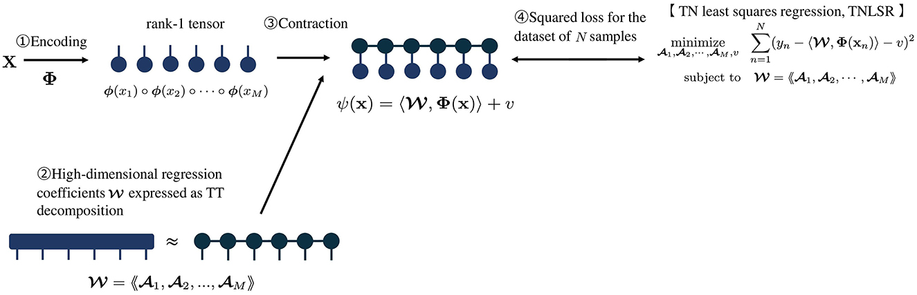
Figure 1. Overview of least squares regression with TN model [7].

As shown in Figure 1, the large coefficient tensor $\mathcal{W}$ ∈ ℝ^{d×d×⋯ × d} is compactly represented using TT:

$\begin{array}{ll}W=\langle \langle A_1,A_2,...,A_M\rangle \rangle ,& (5)\end{array}$

where $A_j\in {ℝ}^{R_{j-1}\times d\times R_j}$ is the j-th core tensor (TT-core), and R_j is called TT-rank or bond dimension for 1 ≤ j ≤ M − 1 which is an important hyper-parameter for controlling the capacity of TN models. In the core tensors at both ends, R₀ = R_M = 1. A TN model with large TT-ranks has a large capacity, but the computational and training loads are also large.

In summary, let us put a set of all coefficients to learn as θ = ($\mathcal{A}$₁, $\mathcal{A}$₂, ..., $\mathcal{A}$_M, v), then the TN model with θ is denoted by

$\begin{array}{ll}\psi (\text{x}|\theta ):=\langle \langle \langle A_1,A_2,...,A_M\rangle \rangle ,\text{Φ}(\text{x})\rangle +v.& (6)\end{array}$

The TN model is characterized by mapping the features into a very high-dimensional space and performing linear regression in that high-dimensional feature space, while not explicitly carrying out the computations in the high-dimensional space. Φ and $\mathcal{W}$ are very higher-order tensors with d^M entries, but the tensor contraction 〈$\mathcal{W}$, Φ(x)〉 can be computed efficiently and it is not necessary to compute Φ and $\mathcal{W}$ themselves explicitly. This approach helps avoid the curse of dimensionality, which is a key issue of high-dimensional classification models.

2.2 Gradient-based algorithm for tensor network least squares regression

When training data ${\{(x_n,y_n)\}}_{n\in [N]}$ are given, the overall structure of the TN regression is as shown in Figure 1. The regression coefficients [e.g., TT-cores ($\mathcal{A}$₁, ..., $\mathcal{A}$_M)] and the bias v are optimized using squared loss. The optimization problem is expressed as

$\begin{array}{lll}{\displaystyle \underset{\theta }{\text{minimize}}}& {\displaystyle {\sum }_{n\in \left[N\right]}}{(y_n-\psi ({\text{x}}_n|\theta ))}^2.& (7)\end{array}$

We refer this task as tensor network least squares regression (TNLSR). Let the sum of squared losses be denoted as f(θ), the naive gradient descent method is then given by

$\begin{array}{ll}{\theta }^{(t+1)}\leftarrow {\theta }^{(t)}-\mu {\nabla }_{\theta }f({\theta }^{(t)}).& (8)\end{array}$

Here, μ is the learning rate.

In the original work by Stoudenmire and Schwab [7], a sweep algorithm is proposed to optimize the regression coefficients ($\mathcal{A}$₁, $\mathcal{A}$₂, ..., $\mathcal{A}$_M) in a block coordinate descent mannar with truncated SVD. The sweep algorithm sequentially updates two core tensors $\mathcal{A}$_m and $\mathcal{A}$_m+1.

In each step of the sweep, two adjacent core tensors, $\mathcal{A}$_m and $\mathcal{A}$_m+1, are contracted with a common TT rank R_m and merged into a single joint tensor $T_m\in {ℝ}^{R^{m-1}\times d\times d\times R^{m+1}}$. Then, we compute the gradient of the loss function with respect to $\mathcal{T}$_m and update $\mathcal{T}$_m by gradient descent. Using truncated SVD, the matrix form of the updated joint tensor $\mathcal{T}$_m is decomposed into two matrices and their tensorized forms are replaced by new core tensors $\mathcal{A}$_m and $\mathcal{A}$_m+1.

Focusing to optimization with respect to $\mathcal{T}$_m, the inner product term of the TN model can be rewritten as:

$\begin{array}{l}\langle W,\Phi (x)\rangle =\langle \langle \langle A_1,\cdots ,A_m,A_{m+1},\cdots ,A_M\rangle \rangle ,\\ {\varphi }^{(1)}\circ \cdots \circ {\varphi }^{(m)}\circ {\varphi }^{(m+1)}\circ \cdots \circ {\varphi }^{(M)}\rangle & (9)\end{array}$

$\begin{array}{ll}=\langle T_m,{\text{l}}^{(m)}\circ {\varphi }^{(m)}\circ {\varphi }^{(m+1)}\circ {\text{r}}^{(m+1)}\rangle ,& (10)\end{array}$

where we put ${\varphi }^{(j)}:=\varphi (x_j)$, and l^(m) and r^(m+1) are respectively results of the contraction of the left and right sides as shown in Figure 2. In practice, this is calculated in parallel for all samples as

$\begin{array}{ll}\langle W,\text{Φ}({\text{x}}_n)\rangle =\langle T_m,{\text{l}}_n^{(m)}\circ {\varphi }_n^{(m)}\circ {\varphi }_n^{(m+1)}\circ {\text{r}}_n^{(m+1)}\rangle & (11)\end{array}$

Figure 2

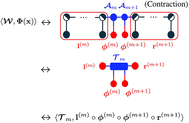
Figure 2. Analysis of TN model for gradient descent in tensor network diagrams [4]. Tensor contraction results in the inner product between $\mathcal{T}$_m and l^(m) ° ϕ^(m) ° ϕ^(m+1) ° r^(m+1). (a) Results of contraction. (b) Entire diagram for all samples.

for all n ∈ [N]. By utilizing this, the gradient of the loss function can be computed as

$\begin{array}{l}\text{Δ}{T}_m=-\frac{\partial f(T_m)}{\partial T_m}={\displaystyle \sum _{n\in [N]}(y_n-\psi (}{x}_n|\theta ))(l_n^{(m)}\circ {\varphi }_n^{(m)}\circ {\varphi }_n^{(m+1)}\\ \circ r_n^{(m+1)}).& (12)\end{array}$

Then, the joint tensor can be updated by gradient descent as $\mathcal{T}$_m ← $\mathcal{T}$_m + μΔ$\mathcal{T}$_m.

Figure 3 shows the image of the entire sweep algorithm. The upper part and the lower part in Figure 3 are called the forward sweep and the backward sweep, respectively. In the forward sweep, the following steps are performed:

$\begin{array}{lll}{T}_m& \leftarrow \langle \langle A_m,A_{m+1}\rangle \rangle ,& (13)\end{array}$

$\begin{array}{lll}{T}_m& \leftarrow T_m+\mu \text{Δ}{T}_m,& (14)\end{array}$

$\begin{array}{ll}\left[\text{U},\text{Σ},\text{V}\right]\leftarrow \text{trSVD}({\text{mat}}_{1,2}(T_m),R_m),& (15)\end{array}$

$\begin{array}{lll}{A}_m& \leftarrow {\text{fold}}_3({\text{U}}^{\top }),& (16)\end{array}$

$\begin{array}{lll}{A}_{m+1}& \leftarrow {\text{fold}}_1(\text{Σ}{\text{V}}^{\top }),& (17)\end{array}$

where trSVD(mat_{1, 2}($\mathcal{T}$_m), R_m) represents the truncated SVD with rank R_m of the input matrix ${\mathrm{\text{mat}}}_{1,2}(T_m)\in {ℝ}^{R_{m-1}d\times d{R}_{m+1}}$. The output matrices of trSVD(mat_{1, 2}($\mathcal{T}$_m), R_m) are $\mathbf{\text{U}}\in {ℝ}^{R_{m-1}d\times R_m}$, $\text{Σ}\in {ℝ}^{R_m\times R_m}$, and $\mathbf{\text{V}}\in {ℝ}^{d{R}_{m+1}\times R_m}$, respectively. In the backward sweep, the following steps are performed:

$\begin{array}{lll}{T}_m& \leftarrow \langle \langle A_m,A_{m+1}\rangle \rangle ,& (18)\end{array}$

$\begin{array}{lll}{T}_m& \leftarrow T_m+\mu \text{Δ}{T}_m,& (19)\end{array}$

$\begin{array}{ll}\left[\text{U},\text{Σ},\text{V}\right]\leftarrow \text{trSVD}({\text{mat}}_{1,2}(T_m),R_m),& (20)\end{array}$

$\begin{array}{lll}{A}_m& \leftarrow {\text{fold}}_3(\text{Σ}{\text{U}}^{\top }),& (21)\end{array}$

$\begin{array}{lll}{A}_{m+1}& \leftarrow {\text{fold}}_1({\text{V}}^{\top }).& (22)\end{array}$

Figure 3

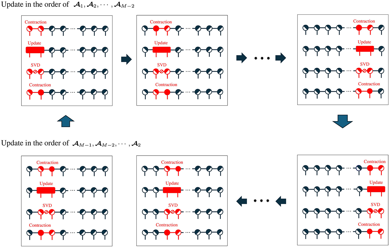
Figure 3. Overall sweep process in TNLSR-GD-SVD. The upper half represents a forward sweep, and the lower half represents a backward sweep. Each block consists of contraction of two core tensor to construct a jonit tensor, the update of the joint tensor based on the gradient descent, decomposition of the updated joint tensor with SVD, and replacement of two core tensors.

In the forward sweep, updates are performed in the order $\mathcal{A}$₁, $\mathcal{A}$₂, ⋯ , $\mathcal{A}$_M−2, and in the backward sweep, updates are performed in the order $\mathcal{A}$_M−1, $\mathcal{A}$_M−2, ⋯ , $\mathcal{A}$₂.

In this algorithm, as an option, R_m in the truncated SVD can be adaptively changed for each iteration. For example, one approach is to determine R_m based on the singular values obtained via SVD, removing components with small singular values. It should be noted that truncated SVD can cause convergence to become unstable. This is because truncated SVD is a process for parameter compression and rank determination, which is not related to minimizing the cost function. In most cases, the cost function increases due to perturbations caused by parameter compression using truncated SVD. The convergence behavior becomes unstable because the cost function decreases due to gradient descent and increases due to truncated SVD alternately.

In this paper, we refer to the above algorithm as TNLSR-GD-SVD. Although TNLSR-GD-SVD has been reported with some success in the classification task of MNIST [7], some problems remain. First, the slow convergence of gradient-based methods can be problematic. In general, many iterations are required for the gradient method to reach the minimum since it is the first-order method. Additionally, tuning an appropriate learning rate is necessary and making efficient convergence challenging. Second, instability in learning due to vanishing gradients is another issue. When the gradient vanishes, the changes in parameters to be updated by the optimization algorithm become negligible, which can lead to training failure. Third, the use of squared loss is inappropriate for classification problems. In general, logistic loss is more suitable for learning classifiers.

2.3 Motivation

In this study, we propose algorithms for learning TN models based on alternating least squares (ALS), which is the workhorse algorithm for tensor decompositions [6, 21–26]. By employing ALS, the monotonic decrease of the objective function is guaranteed without tuning hyperparameters, leading to stabler and faster convergence.

In the case of classification, it is appropriate to minimize the logistic loss

$\begin{array}{r}h(\theta )={\displaystyle \sum _{n\in \left[N\right]}}-y_{n}log\left[\frac{1}{1+e^{-\psi ({\text{x}}_n|\theta )}}\right]\\ -(1-y_n)log\left[\frac{e^{-\psi ({\text{x}}_n|\theta )}}{1+e^{-\psi ({\text{x}}_n|\theta )}}\right]& (23)\end{array}$

rather than squared loss. In this paper, we refer to this task as tensor network logistic regression (TNLR). TNLR can be solved in the same mannar as TNLSR-GD-SVD by replacing the gradient calculation (Equation 12) for logistic loss, we refer to this as TNLR-GD-SVD. However, the problems of gradient descent also remain.

In this study, we propose a new optimization algorithm to address this problem using ALS. Instead of directly minimizing logistic loss (Equation 23), the proposed method introduces an auxiliary function that provides an upper bound and minimizes logistic loss by minimizing the auxiliary function. This approach is generally known as the majorization-minimization (MM) algorithm [27, 28]. For the derivation of the auxiliary function, we employ the PG augmentation [19, 20]. It results in the two-step algorithm of (E-step) computing expectation of latent variable, (M-step) updating θ to minimize weighted least squares by ALS. The derived optimization algorithm can be interpreted as a kind of EM-ALS [29, 30]. Due to the properties of MM and ALS, monotonic decrease (non-increase) of the logistic loss can be guaranteed.

3 Alternating least squares for tensor network least squares regression

3.1 Subproblems and their solutions

In this section, we consider solving the problem shown in Equation 7 by using the ALS algorithm. First, we do not consider the joint core tensor $\mathcal{T}$_m here and update each core tensor $\mathcal{A}$_m one by one. ALS algorithm updates each core tensor $\mathcal{A}$₁, $\mathcal{A}$₂, ⋯ , $\mathcal{A}$_M alternately through suboptimization. The update rules are given by

$\begin{array}{ll}(A_m,v)\leftarrow {\displaystyle \underset{A_m,v}{argmin}}f(A_m,v),m=1,\dots ,M.& (24)\end{array}$

Let us consider to reorganize the objective function by seeing ($\mathcal{A}$_m, v) as optimization parameters for specific m. When optimizing the squared loss (Equation 7) as a sub-optimization problem for the m-th core tensor $\mathcal{A}$_m, the inner product of the TN model is transformed as

$\begin{array}{l}\langle W,\Phi (x)\rangle =\langle \langle \langle A_1,\cdots ,A_m,\cdots ,A_M\rangle \rangle ,{\varphi }_n^{(1)}\circ \cdots \circ {\varphi }^{(m)}\\ \circ \cdots \circ {\varphi }^{(M)}\rangle \\ =\langle A_m,l^{(m)}\circ {\varphi }^{(m)}\circ r^{(m)}\rangle ,& (25)\end{array}$

where we put ${\varphi }^{(j)}:=\varphi (x_j)$, and l^(m) and r^(m) are respectively results of the contraction of the left and right sides as shown in Figure 4a. In practice, this is calculated in parallel for all samples as

$\begin{array}{ll}\langle W,\text{Φ}({\text{x}}_n)\rangle =\langle A_m,{\text{l}}_n^{(m)}\circ {\varphi }_n^{(m)}\circ {\text{r}}_n^{(m)}\rangle & (26)\end{array}$

for all n ∈ [N]. Let the matrices L^(m), Φ^(m), R^(m) and the vector y be defined as

$\begin{array}{l}{\text{l}}^{(m)}=\left[{\text{l}}_1^{(m)},{\text{l}}_2^{(m)},\cdots ,{\text{l}}_N^{(m)}\right]\in {ℝ}^{R_{m-1}\times N},\\ {\text{Φ}}^{(m)}=\left[{\varphi }_1^{(m)},{\varphi }_2^{(m)},\cdots ,{\varphi }_N^{(m)}\right]\in {ℝ}^{d\times N},\\ {\text{r}}^{(m)}=\left[{\text{r}}_1^{(m)},{\text{r}}_2^{(m)},\cdots ,{\text{r}}_N^{(m)}\right]\in {ℝ}^{R_m\times N},\\ \text{y}={\left[y_1,y_2,\cdots ,y_N\right]}^{\top }\in {ℝ}^N,& (27)\end{array}$

then the objective function of the sub-optimization problem in Equation 7 can be written as

$\begin{array}{ll}f(A_m,v)=||\text{y}-{({\text{l}}^{(m)}\odot {\text{Φ}}^{(m)}\odot {\text{R}}^{(m)})}^{\top }\text{vec}(A_m)-v\text{1}{||}_2^2.& (28)\end{array}$

Figure 4

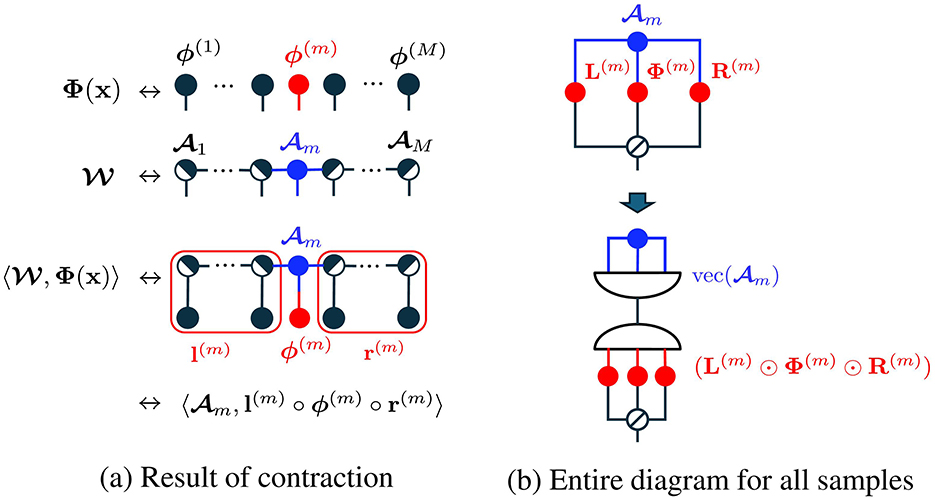
Figure 4. Analysis of TN model for ALS in tensor network diagrams [4]. Tensor contraction results in the inner product between $\mathcal{A}$_m and l^(m) ° ϕ^(m) ° r^(m). Inserting a vectorization-tensorization operation, equivalent to identity mapping, results in the matrix-vector form with Khatri-Rao products. The node with diagonal line represents a superdiagonal tensor.

Above transformation can be graphically verified by using tensor network diagram shown in Figure 4b.

Now, the objective function (Equation 28) can be clearly seen as a standard least squares problem. Let us put ${\beta }_m={\left[\mathrm{\text{vec}}{(A_m)}^{\top },v\right]}^{\top }$ and ${\mathbf{\text{Z}}}_m=\left[{({\mathbf{\text{L}}}^{(m)}\odot {\text{Φ}}^{(m)}\odot {\mathbf{\text{R}}}^{(m)})}^{\top },\mathbf{\text{1}}\right]$, then the solution is given by

$\begin{array}{ll}{\widehat{\beta }}_m={({\text{Z}}_m^{\top }{\text{Z}}_m)}^{-1}{\text{Z}}_m^{\top }\text{y}.& (29)\end{array}$

$\mathcal{A}$_m and v can be updated by replacing with corresponding entries from ${\widehat{\beta }}_m$. The squared loss (Equation 7) takes the form of a quadratic function for each parameter, and the update rule through sub-optimization is given in closed form, ensuring that the error always decreases (monotonic nonincrease). Compared with gradient-based optimization algorithms, which require the careful tuning of learning rate, ALS can stably reduce the objective function without any hyperparameters.

In practice for stabilizing matrix computations, we use

$\begin{array}{ll}{\widehat{\beta }}_m^{(ϵ)}={({\text{Z}}_m^{\top }{\text{Z}}_m+ϵ\text{I})}^{-1}{\text{Z}}_m^{\top }\text{y}& (30)\end{array}$

with small ϵ > 0. This corresponds to adding a Tikhonov regularization, which adds the sum of squares of the regression coefficients $ϵ||{\beta }_m{||}_2^2$ as a penalty term to the objective function (Equation 28).

3.2 Optimization with orthogonalization and sweep

In the optimization of TNs, there is an issue of scale non-uniqueness regarding core tensors. For example, for any c≠0, we have:

$\begin{array}{l}W=\langle A_1,\cdots ,A_i,\cdots ,A_j,\cdots ,A_M\rangle \\ =\langle A_1,\cdots ,c{A}_i,\cdots ,c^{-1}{A}_j,\cdots ,A_M\rangle .& (31)\end{array}$

Here, increasing c results in an increase in the value of c$\mathcal{A}$_i, while $c^{-1}{A}_j$ decreases, but it does not affect the value of the objective function f(θ). If such scale biases become extreme, numerical calculations can become unstable.

To address this problem, in the optimization of TNs, orthogonalization and sweep are combined with ALS [24]. Figure 5 shows the image of the entire algorithm. In this paper, we refer to the above algorithm as TNLSR-ALS-QR. The upper and lower parts are called the forward sweep and the backward sweep, respectively. The half black and half white circular objects represent the left-orthogonal or right-orthogonal tensors.

Figure 5

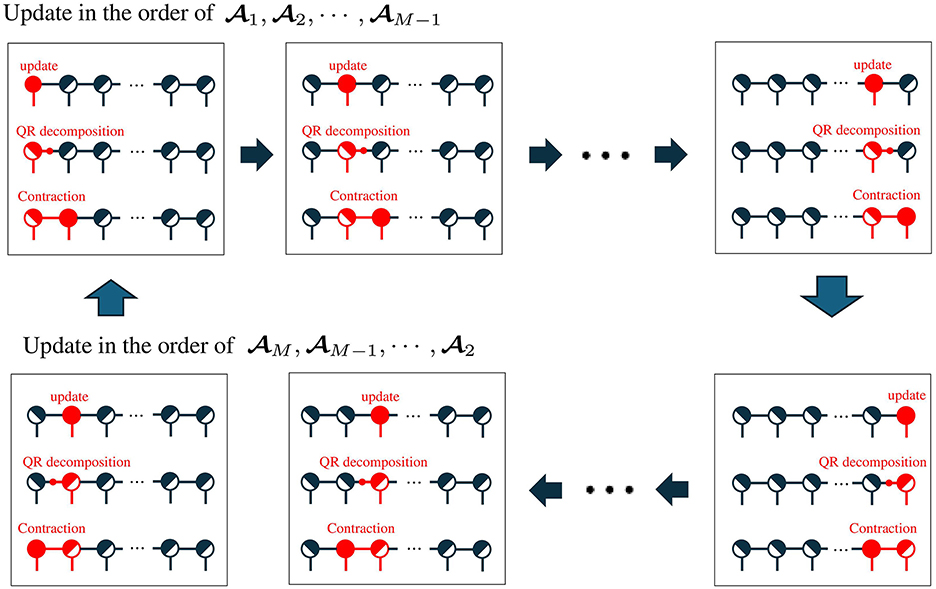
Figure 5. Overall sweep process in ALS. The upper half represents a forward sweep, and the lower half represents a backward sweep. Each block consists of the update of core tensor based on the least squares, orthogonalization by QR decomposition, and contraction of the residual components and the next core tensor.

At the start of the optimization, we assume that all tensors except $\mathcal{A}$₁ are right-orthogonal tensors. In the forward sweep, we update core tensors in the order of $\mathcal{A}$₁, $\mathcal{A}$₂, ⋯ , $\mathcal{A}$_M−1, and update rules for the m-th core tensor is given by

$\begin{array}{ll}(A_m,v)\leftarrow {\displaystyle \underset{A_m,v}{argmin}}f(A_m,v),& (32)\end{array}$

$\begin{array}{lll}\left[\text{Q},\text{R}\right]& \leftarrow \text{QR}({\text{mat}}_3{(A_m)}^{\top }),& (33)\end{array}$

$\begin{array}{lll}{A}_m& \leftarrow {\text{fold}}_3({\text{Q}}^{\top }),& (34)\end{array}$

$\begin{array}{lll}{A}_{m+1}& \leftarrow {\text{fold}}_1(\text{R}{\text{mat}}_1(A_{m+1})),& (35)\end{array}$

where $\mathrm{\text{QR}}({\mathrm{\text{mat}}}_3{(A_m)}^{\top })$ represents the QR decomposition of the input matrix ${\mathrm{\text{mat}}}_3{(A_m)}^{\top }\in {ℝ}^{R_{m-1}d\times R_m}$. The QR decomposition results in a colum orthogonal matrix $\text{Q}\in {ℝ}^{R_{m-1}d\times R_m}$ and an upper triangular matrix $\text{r}\in {ℝ}^{R_m\times R_m}$. After the ALS update, the updated core tensor $\mathcal{A}$_m is separated into a left-orthogonal tensor ${\mathrm{\text{fold}}}_3({\text{Q}}^{\top })$ and residual components R by QR decomposition. The residual components are integrated into the next core tensor (i.e., $\mathcal{A}$_m+1). At the end of the forward sweep, all core tensors except $\mathcal{A}$_M are left-orthogonal. Note that the QR decomposition in this algorithm does not change the value of the objective function.

In the backward sweep, we update core tensors in the order of $\mathcal{A}$_M, $\mathcal{A}$_M−1, ⋯ , $\mathcal{A}$₂, and update rule for the m-th core tensor is given by

$\begin{array}{ll}(A_m,v)\leftarrow {\displaystyle \underset{A_m,v}{argmin}}f(A_m,v),& (36)\end{array}$

$\begin{array}{lll}\left[\text{Q},\text{R}\right]& \leftarrow \text{QR}({\text{mat}}_1{(A_m)}^{\top }),& (37)\end{array}$

$\begin{array}{lll}{A}_m& \leftarrow {\text{fold}}_1({\text{Q}}^{\top }),& (38)\end{array}$

$\begin{array}{lll}{A}_{m-1}& \leftarrow {\text{fold}}_3({\text{mat}}_3{(A_{m-1})}^{\top }{\text{R}}^{\top }).& (39)\end{array}$

After the ALS update, the updated core tensor $\mathcal{A}$_m is separated into a right-orthogonal tensor ${\mathrm{\text{fold}}}_1({\text{Q}}^{\top })$ and the residual components R^⊤ by QR decomposition. The residual components are integrated into the previous core tensor $\mathcal{A}$_m−1. At the end of the backward sweep, all core tensors except $\mathcal{A}$₁ are right-orthogonal.

3.3 Adaptive rank determination

TT-ranks or bond dimensions R_m are important hyperparameters to control the capacity of the TN models and appropriate rank settings are different for different data in general. In Sections 3.1, 3.2, TT ranks are determined prior to optimization and fixed until convergence. However, it is difficult to know the appropriate rank in advance of learning. Hence, we consider a method to determine the rank adaptively according to the data while learning. This method is used in TNLSR-GD-SVD [7], and also in modified ALS for the standard TT decomposition [24]. In this option, the entire algorithm is almost the same as TNLSR-GD-SVD but only the update rule for $\mathcal{T}$_m is different. We update $T_m\in {ℝ}^{R_{m-1}\times d\times d\times R_{m+1}}$ with the solution of the suboptimization problem, and the TT rank R_m is determined using the singular values of mat_{1, 2}($\mathcal{T}$_m). We refer to this algorithm as TNLSR-ALS-SVD.

3.3.1 Update rules for $\mathcal{T}$_m

The objective function in Equation 7 with respect to $\mathcal{T}$_m can be reorganized as

$\begin{array}{ll}f(T_m,v)=||\text{y}-{({\text{l}}^{(m)}\odot {\text{Φ}}^{(m)}\odot {\text{Φ}}^{(m+1)}\odot {\text{R}}^{(m+1)})}^{\top }vec(T_m)-v\text{1}{||}_2^2.& (40)\end{array}$

Let us put ${\gamma }_m={\left[\mathrm{\text{vec}}{(T_m)}^{\top },v\right]}^{\top }$ and ${\mathbf{\text{Z}}}_{m,m+1}=\left[{({\mathbf{\text{L}}}^{(m)}\odot {\text{Φ}}^{(m)}\odot {\text{Φ}}^{(m+1)}\odot {\mathbf{\text{R}}}^{(m+1)})}^{\top },\mathbf{\text{1}}\right]$, then the optimal solution is given by:

$\begin{array}{ll}{\widehat{\text{γ}}}_{m,m+1}={({\text{Z}}_{m,m+1}^{\top }{\text{Z}}_{m,m+1})}^{-1}{\text{Z}}_{m,m+1}^{\top }\text{y}.& (41)\end{array}$

In practice, we use Tikhonov regularization as

$\begin{array}{ll}{\widehat{\text{γ}}}_{m,m+1}^{(ϵ)}={({\text{Z}}_{m,m+1}^{\top }{\text{Z}}_{m,m+1}+ϵ\text{I})}^{-1}{\text{Z}}_{m,m+1}^{\top }\text{y}.& (42)\end{array}$

3.3.2 Adaptive rank determination with singular values

The TT-rank R_m is determined by using singular values of ${\mathrm{\text{mat}}}_{1,2}(T_m)\in {ℝ}^{R_{m-1}d\times d{R}_{m+1}}$ as

$\begin{array}{ll}{\sigma }_1\ge {\sigma }_2\ge \cdots \ge {\sigma }_D& (43)\end{array}$

where we denote the maximum rank of mat_{1, 2}($\mathcal{T}$_m) by D = min(R_m−1d, dR_m+1).

One of typical methods to determine the rank is to remove weak components with a small threshold ε>0. Hence, the estimated rank is given by ${\widehat{R}}_m=max\left\{r|{\sigma }_r\ge \epsilon \right\}$. Another typical method to determine rank is to apply a threshold 0 < δ ≤ 1 to the cumulative contribution ratio $C_r=\frac{\sum _{i=1}^r{\sigma }_i}{\sum _{i=1}^D{\sigma }_i}$. In this case, the estimated rank is given by ${\widehat{R}}_m=min\left\{r|C_r\ge \delta \right\}$.

It should be noted that when the rank is not fixed but is determined adaptively using truncated SVD, the monotonically decreasing nature of the objective function in ALS is no longer guaranteed. This adverse effect can be mitigated by setting ε to a small value or δ to a large value, but the rank may then become large, leading to large computational cost and overfitting to the data. This tradeoff will also be affected by the Tikhonov regularization.

4 EM algorithm for tensor network logistic regression

4.1 Likelihood function in logistic regression

Minimizing the objective function given by the sum of squared losses can be seen as the maximum likelihood estimation under the assumption that observations y follow a normal distribution with expectation ψ(x|θ). However, this is not appropriate from the perspective of a classification task. In particular, in logistic regression (binary classification), we assume that observations y follow a Bernoulli distribution with expectation $\frac{1}{1+e^{-\psi (\mathbf{\text{x}}|\theta )}}$, and the likelihood function with training samples ${\{(x_n,y_n)\}}_{n\in [N]}$ we want to maximize is given by

$\begin{array}{ll}L(\theta )={\displaystyle \prod _{n=1}^N}{\left(\frac{1}{1+e^{-\psi ({\text{x}}_n|\theta )}}\right)}^{y_n}{\left(\frac{e^{-\psi ({\text{x}}_n|\theta )}}{1+e^{-\psi ({\text{x}}_n|\theta )}}\right)}^{1-y_n}.& (44)\end{array}$

Here, we aim for maximizing the likelihood (Equation 44) or minimizing its negative logarithm (Equation 23) by learning θ using ALS.

4.2 Majorization-minimization with ALS

In this study, we propose to employ majorization-minimization (MM) [28] for the optimization of Equation 44. Let us put the objective function h(θ) = −logL(θ), we introduce auxiliary function g(θ|θ′) which holds the conditions

$\begin{array}{ll}h(\theta )\le g(\theta |{\theta }^{\prime }),h(\theta )=g(\theta |\theta ).& (45)\end{array}$

Using this conditions, the algorithm

$\begin{array}{ll}{\theta }^{(t+1)}={\displaystyle \underset{\theta }{argmin}}g(\theta |{\theta }^{(t)})& (46)\end{array}$

ensures the monotonic decrease of h(θ), as

$\begin{array}{ll}h({\theta }^{(t+1)})\le g({\theta }^{(t+1)}|{\theta }^{(t)})\le g({\theta }^{(t)}|{\theta }^{(t)})=h({\theta }^{(t)}).& (47)\end{array}$

If the minimizer of the auxiliary function g(θ|θ^(t)) is available in a closed form that is efficiently computable at each step (Equation 46), the algorithm becomes highly practical.

4.2.1 Derivation of the auxiliary function

Here, we explain how to derive an appropriate auxiliary function for the logistic regression problem. This can be achieved by applying the Pólya-Gamma (PG) augmentation [19]. PG augmentation is a method primarily proposed for Bayesian statistical modeling in logistic regression. This method introduces latent variables following the PG distribution, which enables efficient sampling from the posterior distribution. In addition, an expectation-maximization algorithm utilizing PG augmentation was proposed by Scott and Sun [20]. Please note that our study is not based on a Bayesian framework, but rather we use a PG augmentation to a maximum likelihood estimation with the MM framework.

Let us put L_n(θ) the n-th contribution to the likelihood function L(θ) = ∏_{n ∈ [N]}L_n(θ), and we aim to obtain its lower-bound function

$\begin{array}{ll}{B}_n(\theta |{\theta }^{\prime })\le L_n(\theta ),B_n(\theta |\theta )=L_n(\theta ).& (48)\end{array}$

The auxirialy function is given by sum of its negative logarithm as

$\begin{array}{ll}g(\theta |{\theta }^{\prime })={\displaystyle \sum _{n\in \left[N\right]}}-log{B}_n(\theta |{\theta }^{\prime }).& (49)\end{array}$

We can see clearly that Equation 49 holds Equation 45.

Applying theoretical results by Polson [19], the n-th contribution of the likelihood function can be transformed and bounded by Jensen's inequality as

$\begin{array}{l}{L}_n(\theta )={\left(\frac{1}{1+e^{-\psi ({\text{x}}_n|\theta )}}\right)}^{y_n}{\left(\frac{e^{-\psi ({\text{x}}_n|\theta )}}{1+e^{-\psi ({\text{x}}_n|\theta )}}\right)}^{1-y_n}=\frac{{(e^{\psi ({\text{x}}_n|\theta )})}^{y_n}}{1+e^{\psi ({\text{x}}_n|\theta )}}\\ =\frac{1}{2}{e}^{{\kappa }_n\psi ({\text{x}}_n|\theta )}{\displaystyle {\int }_0^{\infty }}{e}^{-{\omega }_n\frac{\psi {({\text{x}}_n|\theta )}^2}{2}}p({\omega }_n|1,0)\text{d}{\omega }_n\\ =\frac{{\widehat{\rho }}_n({\theta }^{\prime })}{2}{e}^{{\kappa }_n\psi ({\text{x}}_n|\theta )}{E}_{{\omega }_n~\text{PG}(1,\psi ({\text{x}}_n|{\theta }^{\prime }))}\left[e^{-{\omega }_n\left(\frac{\psi {({\text{x}}_n|\theta )}^2-\psi {({\text{x}}_n|{\theta }^{\prime })}^2}{2}\right)}\right]\\ \ge \frac{{\widehat{\rho }}_n({\theta }^{\prime })}{2}{e}^{{\kappa }_n\psi ({\text{x}}_n|\theta )}{e}^{-{\widehat{\omega }}_n({\theta }^{\prime })\frac{\psi {({\text{x}}_n|\theta )}^2-\psi {({\text{x}}_n|{\theta }^{\prime })}^2}{2}}=:B_n(\theta |{\theta }^{\prime }),& (50)\end{array}$

where ${\kappa }_n:=y_n-\frac{1}{2}$, p(ω_n|b, c) with parameter b > 0, c ∈ ℝ is probability density function of PG distribution, PG(1,0) represents PG distribution with b = 1 and c = 0, and we define

$\begin{array}{ll}{\widehat{\omega }}_n(\theta ):={\text{𝔼}}_{{\omega }_n~\text{PG}(1,\psi ({\text{x}}_n|\theta ))}\left[{\omega }_n\right]=\frac{1}{2\psi ({\text{x}}_n|\theta )}tanh\left(\frac{\psi ({\text{x}}_n|\theta )}{2}\right),& (51)\end{array}$

$\begin{array}{ll}{\widehat{\rho }}_n(\theta ):={\text{𝔼}}_{{\omega }_n~\text{PG}(1,0)}\left\{e^{-{\omega }_n\frac{\psi {({\text{x}}_n|\theta )}^2}{2}}\right\}.& (52)\end{array}$

Clearly, we can see B_n(θ|θ) = L_n(θ), and it satisfies the conditions in Equation 48.

By taking the negative logarithm of B_n, we obtain

$\begin{array}{ll}-log{B}_n(\theta |{\theta }^{(t)})=\frac{1}{2}{\widehat{\omega }}_n({\theta }^{(t)}){\left(\psi ({\text{x}}_n|\theta )-\frac{{\kappa }_n}{{\widehat{\omega }}_n({\theta }^{(t)})}\right)}^2+\text{const},& (53)\end{array}$

and the overall auxiliary function g(θ|θ^(t)) is given as the form of weighted least squares:

$\begin{array}{lll}g(\theta |{\theta }^{(t)})& =\frac{1}{2}{\displaystyle \sum _{n\in \left[N\right]}}{\widehat{\omega }}_n({\theta }^{(t)}){\left(\psi ({\text{x}}_n|\theta )-\frac{{\kappa }_n}{{\widehat{\omega }}_n({\theta }^{(t)})}\right)}^2+C,& (54)\end{array}$

where C is a constant term that does not contribute to the optimization. Lastly, we can see that it is an iterative algorithm of expectation maximization (EM) in which the expectation of the latent variable ${\widehat{\omega }}_n({\theta }^{(t)})$ is computed based on the current coefficient values θ^(t) by Equation 51, and the resulting ${\widehat{\omega }}_n({\theta }^{(t)})$ is used as a weight coefficient to minimize the weighted least squares (Equation 54).

4.2.2 EM-ALS algorithm

From Equation 46 and Equation 54, the EM algorithm can be obtained as

$\begin{array}{ll}{\widehat{\omega }}_n^{(t)}=\frac{1}{2\psi ({\text{x}}_n|{\theta }^{(t)})}tanh\left(\frac{\psi ({\text{x}}_n|{\theta }^{(t)})}{2}\right)\text{for all }n\in \left[N\right],& (55)\end{array}$

$\begin{array}{ll}{\theta }^{(t+1)}={\displaystyle \underset{\theta }{argmin}}{\displaystyle \sum _{n\in \left[N\right]}}{\widehat{\omega }}_n^{(t)}{\left(\psi ({\text{x}}_n|\theta )-\frac{{\kappa }_n}{{\widehat{\omega }}_n^{(t)}}\right)}^2,& (56)\end{array}$

where updating latent variable ${\widehat{\omega }}_n^{(t)}$ is E-step, and updating coefficients θ^(t+1) is M-step.

We employ the ALS update for the M-step. Objective function of the sub-problem (Equation 56) with respect to ($\mathcal{A}$_m, v) can be transformed as

$\begin{array}{l}g(A_m,v|{\theta }^{(t)})=||{\text{Ω}}_t^{\frac{1}{2}}(\text{κ}\oslash {\omega }_t)-{\text{Ω}}_t^{\frac{1}{2}}{({\text{l}}^{(m)}\odot {\text{Φ}}^{(m)}\odot {\text{R}}^{(m)})}^{\top }\text{vec}(A_m)\\ +v{\text{Ω}}_t^{\frac{1}{2}}\text{1}{||}_2^2,& (57)\end{array}$

where we put ${\text{Ω}}_t=\mathrm{\text{diag}}({\widehat{\omega }}_1^{(t)},{\widehat{\omega }}_2^{(t)},...,{\widehat{\omega }}_N^{(t)})\in {ℝ}^{N\times N}$, ${\omega }_t={\left[{\widehat{\omega }}_1^{(t)},{\widehat{\omega }}_2^{(t)},...,{\widehat{\omega }}_N^{(t)}\right]}^{\top }\in {ℝ}^N$, $\text{κ}={\left[{\kappa }_1,{\kappa }_2,...,{\kappa }_N\right]}^{\top }\in {ℝ}^N$, and ⊘ stands for entry-wise division. This is almost the same form as Equation 28, and the minimizer is given in closed form as

$\begin{array}{ll}{\widehat{\beta }}_m={({\text{Z}}_m^{\top }{\text{Ω}}_t{\text{Z}}_m)}^{-1}{\text{Z}}_m^{\top }(\text{κ}\oslash {\omega }_t).& (58)\end{array}$

Then θ^(t+1) can be updated by replacing the appropriate entries with ${\widehat{\beta }}_m$. In practice, we use

$\begin{array}{ll}{\widehat{\beta }}_m^{(ϵ)}={({\text{Z}}_m^{\top }{\text{Ω}}_t{\text{Z}}_m+ϵ\text{I})}^{-1}{\text{Z}}_m^{\top }(\text{κ}\oslash {\omega }_t)& (59)\end{array}$

with small ϵ > 0 for stable matrix computation.

The overall algorithm is shown in Algorithm 1. We refer to the proposed algorithm as TNLR-EMALS-QR. This algorithm is structured by combining the sweep with QR and EM-ALS, where the parameter θ is divided into M blocks, orthogonalization using QR decomposition at each update, forward sweep and backward sweep. Optionally, it is possible to introduce an adaptive rank algorithm in a similar way to TNLSR-ALS-SVD. We call this TNLR-EMALS-SVD.

Algorithm 1

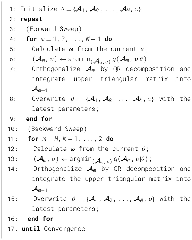
Algorithm 1. TNLR-EMALS-QR: EM-ALS algorithm for TN logistic regression.

4.3 Extension to multi-class classification

4.3.1 Design of TN models

This section discusses how to extend the TN model for multi-class classification. Thus, let us consider a problem to obtain a function: ψ(·|θ):ℝ^M → ℝ^K which satisfies

$\begin{array}{ll}\text{y}\simeq a\circ \psi (\text{x}|\theta ),& (60)\end{array}$

where x ∈ ℝ^M represents pattern, y∈{0, 1}^K represents its one-hot encoded label, and a:ℝ^K → [0, 1]^K is some non-linear activation function.

A naive choice of activation function for multi-class classification is softmax, and cross entropy loss is minimized for learning θ. In this case, gradient-based optimization is possible, but tuning the learning rate is difficult and the convergence is inefficient. Here, PG augmentation can be applied to the above problem setting [20], but this is not a good method for the TN model. The PG augmentation for the multi-class problem proposed by Scott and Sun [20] requires that each channel of output ψ(x|θ) be calculated from separated independent coefficients: $\psi (\mathbf{\text{x}}|{\theta }_1,{\theta }_2,...,{\theta }_K)={\left[\begin{array}{cccc}\psi (\mathbf{\text{x}}|{\theta }_1)& \psi (\mathbf{\text{x}}|{\theta }_2)& \cdots & \psi (\mathbf{\text{x}}|{\theta }_K)\end{array}\right]}^{\top }$. This means learning K TN models separately, which is not practical.

In this study, we propose a more practical method for learning single TN model in multi-class classification. An overview of the proposed method is shown in Figure 6. In the proposed method, similar to Stoudenmire's TN model [7], a mode of length K is added to only one core tensor in the TT decomposition. This is much easier than constructing K TT decompositions. The TN model for multi-class classification is given by

$\begin{array}{ll}\psi (\text{x}|\theta )=\langle \langle A_1,A_2,...,A_M\rangle \rangle \times \text{Φ}(\text{x})+\text{V}\in {ℝ}^K,& (61)\end{array}$

where × stands for the corresponding tensor contraction operation and θ = ($\mathcal{A}$₁, $\mathcal{A}$₂, ..., $\mathcal{A}$_M, v). Note that 〈〈$\mathcal{A}$₁, $\mathcal{A}$₂, ..., $\mathcal{A}$_M〉〉 × Φ(x) outputs a K-dimensional vector and bias v is also a K-dimensional vector.

Figure 6

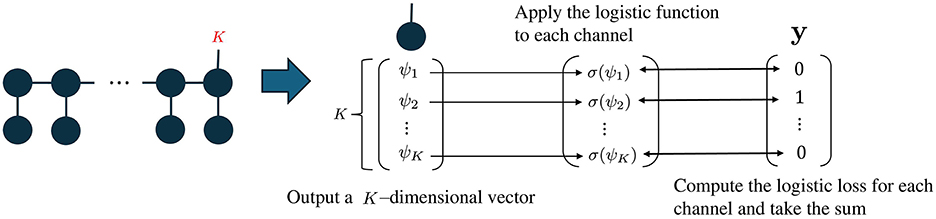
Figure 6. Image of a multi-class classification model with TN. Additional mode of length K representing the number of classes is with the right-end core tensor $\mathcal{A}$_M. The contraction with Φ(x) results in a K-dimensional vector. The logistic loss is calculated for each output dimension.

Furthermore, we employ entry-wise logistic sigmoid for activation function:

$\begin{array}{ll}a(\text{Z})=\left[\begin{array}{c}\sigma (z_1)\\ \sigma (z_2)\\ ⋮\\ \sigma (z_K)\end{array}\right]& (62)\end{array}$

for $\mathbf{\text{z}}=\left[z_1,z_2,...,z_K\right]\in {ℝ}^K$, where $\sigma (z):=\frac{1}{1+e^{-z}}$ is logistic sigmoid function. Coefficients θ is learned with training samples ${\{(x_n,y_n)\}}_{n\in [N]}$ by minimizing sum of logistic loss for all channels as

$\begin{array}{l}{\displaystyle \sum _{n\in \left[N\right]}}{\displaystyle \sum _{k\in \left[K\right]}}-y_{k,n}log\left[\frac{1}{1+e^{-{\psi }_k({\text{x}}_n|\theta )}}\right]\\ -(1-y_{k,n})log\left[\frac{e^{-{\psi }_k({\text{x}}_n|\theta )}}{1+e^{-{\psi }_k({\text{x}}_n|\theta )}}\right],& (63)\end{array}$

where y_{k, n} stands for the k-th entry of y_n and ψ_k(x_n|θ) is the k-th output of ψ(x_n|θ). Since Equation 63 is the sum of logistic losses for individual K classes, the PG augmentation discussed in Section 4 can be applied directly to obtain its auxiliary function.

The approach using the multichannel logistic function can be interpreted as a model where each channel independently generates either 0 or 1. In this approach, it is assumed that each label y_{k, n} (k-th channel of y_n) follows a Bernoulli distribution with expectation ψ_k(x_n|θ) independently. Consequently, the label can contain multiple ones in a vector under the assumption, such as [1, 0, 0, 1, 0, ⋯ ], making it suitable for applications beyond classification. Specifically, this approach can also be applied to tasks in which independent attributes are assigned to each channel of the data. On the other hand, this model has an important limitation: Since the outputs are independent across channels, it does not guarantee consistency, such as ensuring that the sum of output values equals 1. Therefore, careful consideration is required when interpreting them as probability values.

4.3.2 EM-ALS for learning multi-class TN classifiers

From Equation 63, auxiliary function can be directly derived by applying PG augmentation to individual k-th channels one-by-one. This results in the following EM algorithm:

$\begin{array}{ll}{\widehat{\omega }}_{k,n}^{(t)}=\frac{1}{2{\psi }_k({\text{x}}_n|{\theta }^{(t)})}tanh\left(\frac{{\psi }_k({\text{x}}_n|{\theta }^{(t)})}{2}\right)\text{for all }n\in \left[N\right],k\in \left[K\right],& (64)\end{array}$

$\begin{array}{ll}{\theta }^{(t+1)}={\displaystyle \underset{\theta }{argmin}}{\displaystyle \sum _{n\in \left[N\right]}}{\displaystyle \sum _{k\in \left[K\right]}}{\widehat{\omega }}_{k,n}^{(t)}{\left({\psi }_k({\text{x}}_n|\theta )-\frac{{\kappa }_{k,n}}{{\widehat{\omega }}_{k,n}^{(t)}}\right)}^2,& (65)\end{array}$

where ${\kappa }_{k,n}:=y_{k,n}-\frac{1}{2}$.

Next, we reorganize the objective function with respect to $\mathcal{A}$_m and v as sub-optimization parameters. Here, we assume that the additional mode of length K is with M-th core tensor $\mathcal{A}$_M. Then the size of $\mathcal{A}$_M is (R_M−1, d, K). The term of tensor contraction in ψ(x_n|θ) can be transformed as

$\begin{array}{l}\langle \langle A_1,A_2,...,A_M\rangle \rangle \times \text{Φ}({\text{x}}_n)=A_m\times ({\text{l}}_n^{(m)}\circ {\varphi }_n^{(m)}\circ {\text{R}}_n^{(m)})\\ ={({\text{l}}_n^{(m)}\otimes {\varphi }_n^{(m)}\otimes {\text{R}}_n^{(m)})}^{\top }\text{vec}(A_m),& (66)\end{array}$

where ${\text{l}}_n^{(m)}\in {ℝ}^{R_{m-1}}$, ${\varphi }_n^{(m)}\in {ℝ}^d$, and ${\text{r}}_n^{(m)}\in {ℝ}^{R_m\times K}$ are results of contraction as shown in Figure 7. Note that ${\text{r}}^{(m)}\in {ℝ}^{R_m\times K}$ is a matrix which is different from a case of binary classification. The entire objective function of the sub-optimization problem can be expressed as

$\begin{array}{ll}\begin{array}{l}g(A_m,v|{\theta }^{(t)})={\Vert {\Omega }_t^{\frac{1}{2}}(\kappa \oslash {\omega }_t)-{\Omega }_t^{\frac{1}{2}}{B}_m\mathrm{vec}(A_m)-{\Omega }_t^{\frac{1}{2}}Kv\Vert }_2^2,\hfill \end{array}& (67)\end{array}$

where

$\begin{array}{ll}\kappa =\text{vec}\left[\begin{array}{cccc}{\kappa }_{1,1}& {\kappa }_{2,2}& \cdots & {\kappa }_{1,N}\\ {\kappa }_{2,1}& {\kappa }_{2,2}& \cdots & {\kappa }_{2,N}\\ ⋮& ⋮& \ddots & ⋮\\ {\kappa }_{K,1}& {\kappa }_{K,2}& \cdots & {\kappa }_{K,N}\end{array}\right]\in {ℝ}^{KN},& (68)\end{array}$

$\begin{array}{ll}{\omega }_t=\text{vec}\left[\begin{array}{cccc}{\widehat{\omega }}_{1,1}^{(t)}& {\widehat{\omega }}_{2,2}^{(t)}& \cdots & {\widehat{\omega }}_{1,N}^{(t)}\\ {\widehat{\omega }}_{2,1}^{(t)}& {\widehat{\omega }}_{2,2}^{(t)}& \cdots & {\widehat{\omega }}_{2,N}^{(t)}\\ ⋮& ⋮& \ddots & ⋮\\ {\widehat{\omega }}_{K,1}^{(t)}& {\widehat{\omega }}_{K,2}^{(t)}& \cdots & {\widehat{\omega }}_{K,N}^{(t)}\end{array}\right]\in {ℝ}^{KN},& (69)\end{array}$

$\begin{array}{ll}{\text{Ω}}_t=\text{diag}({\omega }_t)\in {ℝ}^{KN\times KN},& (70)\end{array}$

$\begin{array}{ll}{\text{B}}_m=\left[\begin{array}{c}{\left({\text{l}}_1^{(m)}\otimes {\varphi }_1^{(m)}\otimes {\text{R}}_1^{(m)}\right)}^{\top }\\ {\left({\text{l}}_2^{(m)}\otimes {\varphi }_2^{(m)}\otimes {\text{R}}_2^{(m)}\right)}^{\top }\\ ⋮\\ {\left({\text{l}}_N^{(m)}\otimes {\varphi }_N^{(m)}\otimes {\text{R}}_N^{(m)}\right)}^{\top }\end{array}\right]\in {ℝ}^{KN\times R_{m-1}d{R}_m},& (71)\end{array}$

$\begin{array}{ll}\text{K}=\left[\begin{array}{c}\begin{array}{c}{\text{I}}_{K\times K}\\ {\text{I}}_{K\times K}\\ ⋮\\ {\text{I}}_{K\times K}\end{array}\end{array}\right]\in {ℝ}^{KN\times K}.& (72)\end{array}$

Defining the optimization parameter as ${\beta }_m={\left[\mathrm{\text{vec}}{(A_m)}^{\top },{\text{V}}^{\top }\right]}^{\top }$, the optimal solution for β_m in the auxiliary function (Equation 67) is given by

$\begin{array}{ll}{\widehat{\beta }}_m={({\text{Z}}_m^{\top }{\text{Ω}}_t{\text{Z}}_m)}^{-1}{\text{Z}}_m^{\top }(\text{κ}\oslash {\omega }_t),& (73)\end{array}$

where Z_m = [B_m, K]. For the same reason as in the binary classification case, Tikhonov regularization is applied as

$\begin{array}{ll}{\widehat{\beta }}_m^{(ϵ)}={({\text{Z}}_m^{\top }{\text{Ω}}_t{\text{Z}}_m+ϵ\text{I})}^{-1}{\text{Z}}_m^{\top }(\text{κ}\oslash \omega ).& (74)\end{array}$

Figure 7

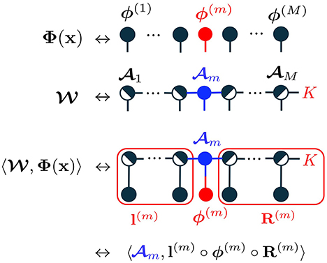
Figure 7. Multi-class TN model of K classes in tensor network diagrams. A class mode of length K is added to the right-end core tensor. The class mode remains in R^(m) after contraction.

4.4 Computational complexity

Here we show the computational complexity of the main processes in the tensor network model. First, the standard inference is given by the inner product of two low-rank tensors and is $\mathcal{O}$(dR²M) where M is the dimension of x, d is the local dimension, R is the rank (assuming R_m = R for all m) and K is the number of classes (assuming K < R).

In learning TN models, the computational complexity for one iteration of GD-QR is $\mathcal{O}$(dR²MNK). In the case of GD-SVD, it is $\mathcal{O}$(dR²(MNK + d²R)) because it requires singular value decomposition of the matrix of size (dR, dR). The computational complexity of ALS-QR is $\mathcal{O}$(dR²(MNK + d²R⁴)) because it is necessary to solve a normal equation of dimension dR². In the same way, the computational complexity of ALS-SVD is $\mathcal{O}$(dR²(MNK + d⁵R⁴)) because it is necessary to solve a normal equation of dimension d²R².

Note that the difference between squared loss and logistic loss makes no difference in computational complexity, just a few extra computations in the case of logistic loss.

5 Experimental results of multi-class classification

In this experiment, we evaluate the behaviors of the proposed algorithm and the performance of the learned classifiers in the classification task of MNIST. The default settings for the TN model are as follows: The original 28 × 28 images were downsampled to 7 × 7 images for the comparison, and the pixel values were normalized to the range [0,1]. The images were vectorized as 49-dimensional vectors x ∈ [0, 1]⁴⁹, and these are inputs into the TN models. The local mapping was based on Equation 4. Let the maximum TT-rank be R and use this as a hyperparameter of the TN model. We compared different optimization algorithms for learning the TN model as shown in Table 1. The learning rates for the descent of the gradient were μ = 10⁻⁴. The tradeoff parameters of the Tikhonov regularization were ϵ = 10⁻⁵.

Table 1

Table 1. Compared algorithms.

5.1 Optimization behavior

Figure 8 shows the comparison of the optimization behaviors for various learning algorithms for the binary classification of MNIST of even and odd numbers. TT-rank is fixed as R = 8 for all algorithms, and the truncated SVD truncates with $\widehat{R}=8$ without adaptive rank determination. For the gradient descent, the learning rates were carefully tuned for better convergence. For reference, the results for two different learning rates are shown in Figure 8. 50 sweep results are shown for gradient-based methods, and 10 sweep results are shown for ALS-based methods.

Figure 8

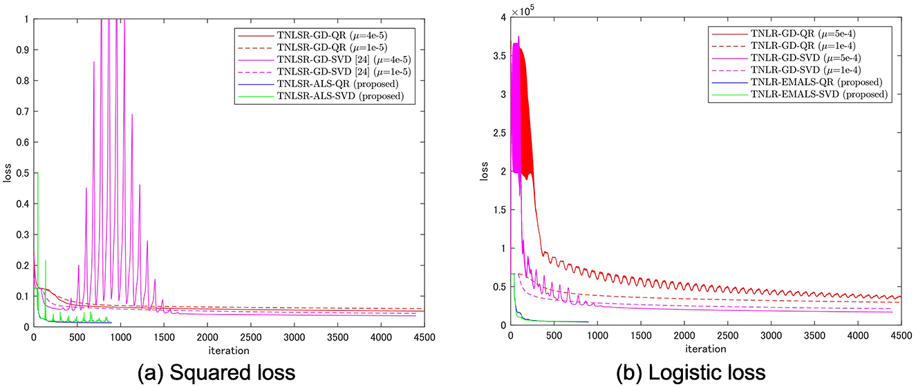
Figure 8. Optimization behaviors of various algorithms for learning TN models. Fifty sweep results are shown for gradient-based methods, and 10 sweep results are shown for ALS-based methods.

In both the squared loss and logistic loss cases, TNLSR-ALS-QR and TNLR-EMALS-QR converged faster and reached better optimal solutions compared to gradient descent. For gradient methods, SVD tends to achieve better final objective values, while for ALS, QR tends to achieve better final objective values. The squared/logistic loss achieved by the proposed methods after 10 sweeps was 0.0133/4.12e3 for ALS-QR and 0.0170/4.67e3 for ALS-SVD. In contrast, the squared/logistic loss achieved by the gradient method after 50 sweeps was 0.0511/2.96e4 for GD-QR and 0.0360/1.69e4 for GD-SVD. The proposed method achieves smaller loss values with fewer sweeps for both loss functions. It can also be seen that the objective function is decreasing monotonically. Gradient descent with a high learning rate will lead to failure, while gradient descent with a low learning rate will converge slowly. Using the sweep algorithm with truncated SVD tends to make optimization unstable (peaks are mixed into the convergence curve).

Table 2 shows average computational time per iteration for various ranks R. The measurements were performed on a workstation with an Intel(R) Xeon(R) CPU E5-2630 v3 @ 2.40GHz with 128 GB memory. In general, we can see that ALS has a higher computational cost than GD. QR-type algorithm is much better than the SVD-type algorithm in computational cost for ALS.

Table 2

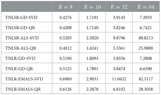
Table 2. Average computational time [sec] per iteration for various ranks R.

5.2 Classification accuracy

The classification accuracy on the MNIST dataset, tested by varying the maximum TT-rank R to 128, is shown in Figure 9 and Table 3. Number of sweeps were 10. For training accuracy, the proposed TNLR-EMALS-QR outperformed all algorithms for all R. This clearly demonstrates that the proposed method works well as an optimization algorithm. It can also be confirmed that minimizing logistic loss is more appropriate than minimizing squared loss in learning classifiers. For test accuracy, the proposed TNLR-EMALS-QR outperformed all algorithms for almost all R. Although the maximum test accuracy is the same for TNLR-EMALS-QR and TNLSR-ALS-QR, we can see that TNLSR-ALS-QR has a stronger tendency to overfit as R increases. These results demonstrate the importance of enabling the optimization of logistic losses.

Figure 9

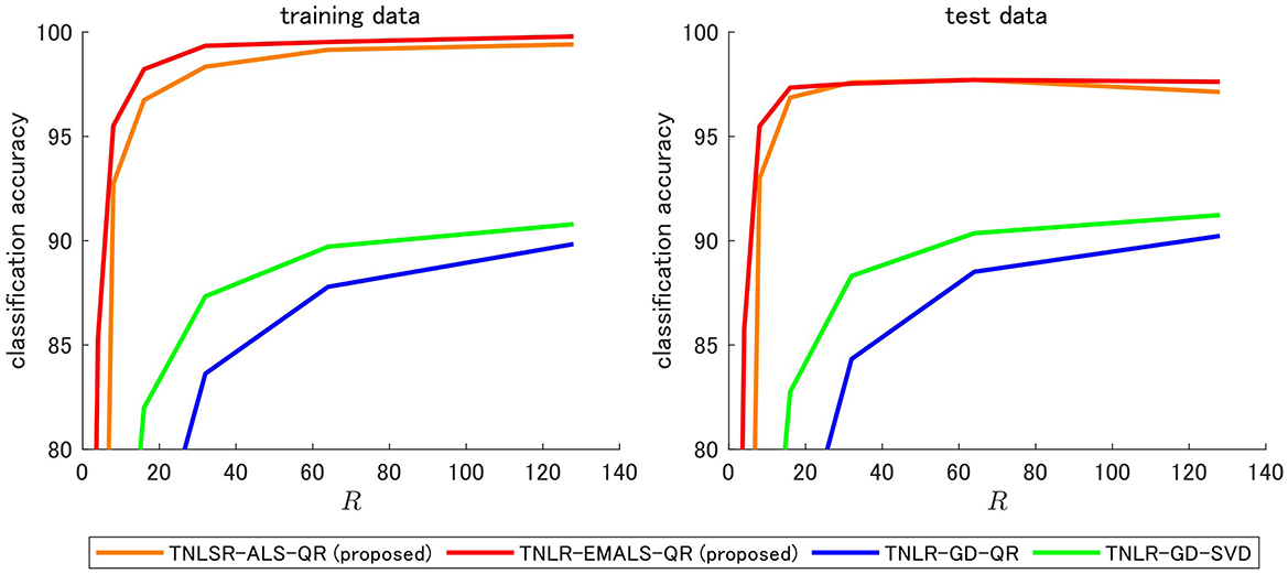
Figure 9. Classification accuracy of MNIST.

Table 3

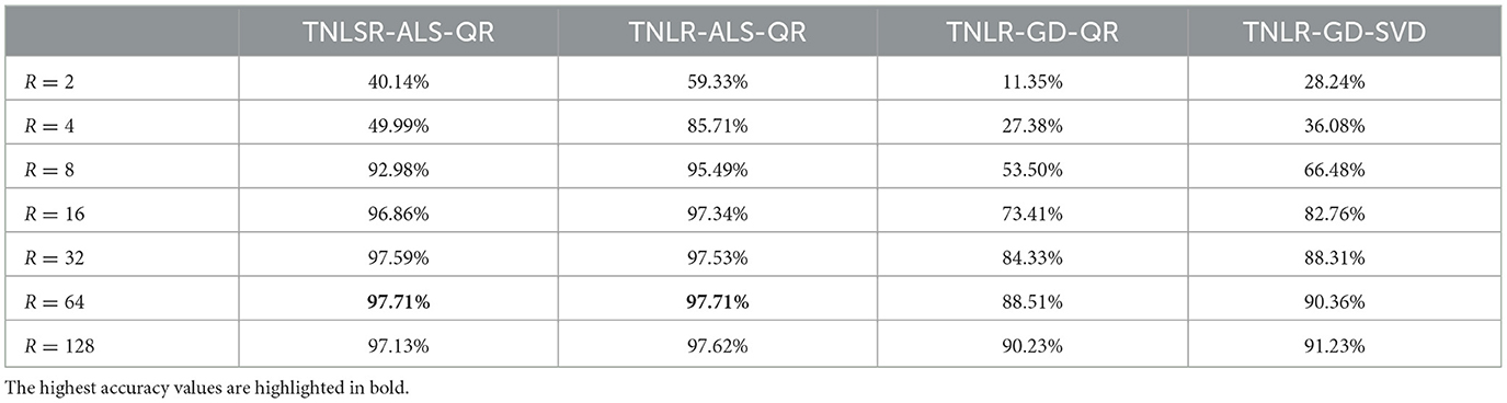
Table 3. Comparison of classification accuracy.

5.3 Hyperparameter sensitivity

5.3.1 Increasing the local dimension d

In this section, we present experimental results for different local dimensions. We used a local mapping with d > 2, which is proposed by Stoudenmire and Schwab [7], as

$\begin{array}{ll}{\varphi }^s(x_j)=\sqrt{\left(\begin{array}{c}d-1\\ s-1\end{array}\right)}{\left(\cos \left(\frac{\pi }{2}{x}_j\right)\right)}^{d-s}{\left(\sin \left(\frac{\pi }{2}{x}_j\right)\right)}^{s-1},& (75)\end{array}$

where s represents the index of entries of ϕ(x_j). It matches Equation 4 with d = 2. Using this function, the multi-class classification of MNIST was performed by changing the local dimension d to 2, 4, 8, and 16.

The results of training and test accuracy are shown in Figure 10. In both squared and logistic losses, high classification performance was observed for d = 2, d = 4, and d = 8. Training and test accuracy both dropped significantly when d = 16. In general, a larger d should increase the expressive power of the TN model. However, the observed drop in training accuracy suggests potential optimization difficulties. For larger d, it may lead to being the landscape of the objective function complex and to stuck poor local minima. Considering the weight of the model and the cost of training, d = 2 seems sufficient for this task.

Figure 10

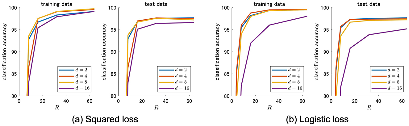
Figure 10. Classification accuracies for different local dimensions.

5.3.2 Adaptive rank determination

Here we demonstrate TNLR-EMALS-SVD with an option of adaptive rank determination using the cumulative contribution rate C_r defined in Section 3.3.2. The initial rank was set to R = 8, and the adaptive rank determination was made in the range of 2 ≤ R ≤ 100. The experiments were carried out with two cumulative contribution rate thresholds: δ = 0.9 and δ = 0.99.

In the case of δ = 0.9, the classification accuracy of the learned classifier was 70.95%. The minimum, median and maximum TT ranks finally obtained were 2, 3, and 7, respectively. Oscillations of the optimization curve are observed. It seems that the threshold was too small.

In the case of δ = 0.99, the classification accuracy of the learned classifier was 96.74%. The minimum, median and maximum TT ranks finally obtained were 2, 21.5, and 100, respectively. The objective function was stably decreased without oscillations. Although it does not achieve the highest accuracy of the fixed rank algorithm, it seems to be still an effective option considering the burden of selecting hyperparameters.

5.3.3 Input dimensions

Although the input dimensionality is not a hyperparameter for the model, it can have a significant impact on the behavior of TN models given the vanishing gradient problem. Here we investigate this by experimenting with different downsampling ratios on MNIST images. Specifically, the input size was varied from a 3 × 3 pixel (9-dimensional vector) to a 14 × 14 pixel (196-dimensional vector), with the pixel size changing by 1 pixel. The TT ranks were set at R = 8, and the local dimension was set at d = 2.

The results are shown in Figure 11. It can be seen that both training and test accuracy increases as the number of input dimensions increases, and then decreases as the number of dimensions increases further. It is intuitive that accuracy improves as input dimensions increase, but the decrease in accuracy is not. Since accuracy decreases in both training and testing, this phenomenon is not due to overfitting, but rather is highly likely that learning is not going well. One of the causes of this may be gradient vanishing. The level of accuracy drop is significant in the gradient method, but it can be seen that the level of accuracy drop is reduced in the proposed algorithms based on ALS.

Figure 11

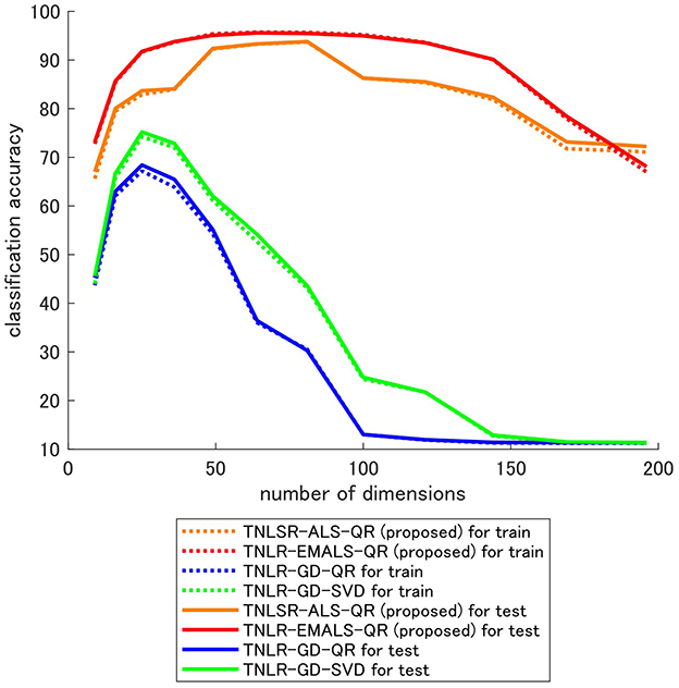
Figure 11. Classification accuracies for different input dimensions.

6 Conclusion

In this study, we propose the use of ALS for supervised learning using TN models rather than gradient descent. We show that squared loss can be directly minimized by ALS and logistic loss can be minimized by EM-ALS with PG augmentation. In experiments, the effectiveness of the proposed algorithms is demonstrated in the classification task of MNIST. For the properties of MM and ALS, the monotonic decrease of the objective function is guaranteed in the proposed algorithms, and convergence is much faster than gradient descent.

Data availability statement

Publicly available datasets were analyzed in this study. This data can be found here: https://pytorch.org/vision/main/generated/torchvision.datasets.MNIST.html.

Author contributions

NY: Writing – review & editing, Writing – original draft. HH: Writing – review & editing. TY: Writing – original draft, Writing – review & editing.

Funding

The author(s) declare that financial support was received for the research and/or publication of this article. This work was partially supported by the Japan Society for the Promotion of Science (JSPS) KAKENHI under Grant 23K28109.

Conflict of interest

The authors declare that the research was conducted in the absence of any commercial or financial relationships that could be construed as a potential conflict of interest.

Generative AI statement

The author(s) declare that Gen AI was used in the creation of this manuscript. The authors used Gen AI for only English proofreading.

Publisher's note

All claims expressed in this article are solely those of the authors and do not necessarily represent those of their affiliated organizations, or those of the publisher, the editors and the reviewers. Any product that may be evaluated in this article, or claim that may be made by its manufacturer, is not guaranteed or endorsed by the publisher.

References

1. Cichocki A, Lee N, Oseledets I, Phan AH, Zhao Q, Mandic DP. Tensor networks for dimensionality reduction and large-scale optimization: part 1 low-rank tensor decompositions. Found Trends Mach Learn. (2016) 9:249–429. doi: 10.1561/2200000059

Crossref Full Text | Google Scholar

2. Cichocki A, Phan AH, Zhao Q, Lee N, Oseledets I, Sugiyama M, et al. Tensor networks for dimensionality reduction and large-scale optimization: part 2 applications and future perspectives. Found Trends Mach Learn. (2017) 9:431–673. doi: 10.1561/9781680832778

Crossref Full Text | Google Scholar

3. Fernández YN, Ritter MK, Jeannin M, Li JW, Kloss T, Louvet T, et al. Learning tensor networks with tensor cross interpolation: new algorithms and libraries. arXiv preprint arXiv:240702454 (2024).

Google Scholar

4. Yokota T. Very basics of tensors with graphical notations: unfolding, calculations, and decompositions. arXiv preprint arXiv:241116094 (2024).

Google Scholar

5. Oseledets IV. Tensor-train decomposition. SIAM J Sci Comput. (2011) 33:2295–317. doi: 10.1137/090752286

Crossref Full Text | Google Scholar

6. Zhao Q, Zhou G, Xie S, Zhang L, Cichocki A. Tensor ring decomposition. arXiv preprint arXiv:160605535 (2016).

Google Scholar

7. Stoudenmire E, Schwab DJ. Supervised learning with tensor networks. In: Advances in Neural Information Processing Systems (2016).

Google Scholar

8. Amiridi M, Kargas N, Sidiropoulos ND. Low-rank characteristic tensor density estimation part I: foundations. IEEE Trans Signal Proc. (2022) 70:2654–68. doi: 10.1109/TSP.2022.3175608

Crossref Full Text | Google Scholar

9. Amiridi M, Kargas N, Sidiropoulos ND. Low-rank characteristic tensor density estimation part II: compression and latent density estimation. IEEE Trans Signal Proc. (2022) 70:2669–80. doi: 10.1109/TSP.2022.3158422

Crossref Full Text | Google Scholar

10. Sengupta R, Adhikary S, Oseledets I, Biamonte J. Tensor networks in machine learning. Eur Mathem Soc Magaz. (2022) 126:4–12. doi: 10.4171/mag/101

Crossref Full Text | Google Scholar

11. Fields C, Fabrocini F, Friston K, Glazebrook JF, Hazan H, Levin M, et al. Control flow in active inference systems-part II: tensor networks as general models of control flow. IEEE Trans Molec Biol Multi-Scale Commun. (2023) 9:246–56. doi: 10.1109/TMBMC.2023.3272158

Crossref Full Text | Google Scholar

12. Memmel E, Menzen C, Schuurmans J, Wesel F, Batselier K. Position: tensor networks are a valuable asset for green AI. In: Proceedings of ICML (2024).

Google Scholar

13. Ye J, Janardan R, Li Q. Two-dimensional linear discriminant analysis. In: Advances in Neural Information Processing Systems (2004).

Google Scholar

14. Tao D, Li X, Wu X, Maybank SJ. General tensor discriminant analysis and gabor features for gait recognition. IEEE Trans Pattern Anal Mach Intell. (2007) 29:1700–15. doi: 10.1109/TPAMI.2007.1096

PubMed Abstract | Crossref Full Text | Google Scholar

15. Lebedev V, Ganin Y, Rakhuba M, Oseledets I, Lempitsky V. Speeding-up convolutional neural networks using fine-tuned CP-decomposition. arXiv preprint arXiv:14126553 (2014).

Google Scholar

16. Novikov A, Podoprikhin D, Osokin A, Vetrov DP. Tensorizing neural networks. In: Proceedings of NeurlPS (2015). p. 28.

Google Scholar

17. Hu EJ, Shen Y, Wallis P, Allen-Zhu Z, Li Y, Wang S, et al. LoRA: low-rank adaptation of large language models. In: Proceedings of ICLR (2022).

Google Scholar

18. Bishop CM, Nasrabadi NM. Pattern Recognition and Machine Learning. Cham: Springer. (2006).

Google Scholar

19. Polson NG, Scott JG, Windle J. Bayesian inference for logistic models using Pólya-Gamma latent variables. J Am Stat Assoc. (2013) 108:1339–49. doi: 10.1080/01621459.2013.829001

Crossref Full Text | Google Scholar

20. Scott JG, Sun L. Expectation-maximization for logistic regression. arXiv preprint arXiv:13060040 (2013).

Google Scholar

21. Carroll JD, Chang JJ. Analysis of individual differences in multidimensional scaling via an N-way generalization of “Eckart-Young” decomposition. Psychometrika. (1970) 35:283–319. doi: 10.1007/BF02310791

Crossref Full Text | Google Scholar

22. Harshman RA. Foundations of the PARAFAC procedure: Models and conditions for an “explanatory” multimodal factor analysis. UCLA Working Paper Phonet. (1970) 16:1–84.

Google Scholar

23. Kroonenberg PM, De Leeuw J. Principal component analysis of three-mode data by means of alternating least squares algorithms. Psychometrika. (1980) 45:69–97. doi: 10.1007/BF02293599

Crossref Full Text | Google Scholar

24. Holtz S, Rohwedder T, Schneider R. The alternating linear scheme for tensor optimization in the tensor train format. SIAM Sci Comput. (2012) 34:A683–713. doi: 10.1137/100818893

Crossref Full Text | Google Scholar

25. Kolda TG, Bader BW. Tensor decompositions and applications. SIAM Rev. (2009) 51:455–500. doi: 10.1137/07070111X

Crossref Full Text | Google Scholar

26. Cichocki A, Mandic D, De Lathauwer L, Zhou G, Zhao Q, Caiafa C, et al. Tensor decompositions for signal processing applications: from two-way to multiway component analysis. IEEE Signal Process Mag. (2015) 32:145–63. doi: 10.1109/MSP.2013.2297439

Crossref Full Text | Google Scholar

27. Kiers HA. Majorization as a tool for optimizing a class of matrix functions. Psychometrika. (1990) 55:417–28. doi: 10.1007/BF02294758

Crossref Full Text | Google Scholar

28. Sun Y, Babu P, Palomar DP. Majorization-minimization algorithms in signal processing, communications, and machine learning. IEEE Trans Signal Proc. (2016) 65:794–816. doi: 10.1109/TSP.2016.2601299

Crossref Full Text | Google Scholar

29. Dempster AP, Laird NM, Rubin DB. Maximum likelihood from incomplete data via the EM algorithm. J R Stat Soc. (1977) 39:1–22. doi: 10.1111/j.2517-6161.1977.tb01600.x

Crossref Full Text | Google Scholar

30. Tomasi G, Bro R. PARAFAC and missing values. Chemometr Intell Labor Syst. (2005) 75:163–80. doi: 10.1016/j.chemolab.2004.07.003

Crossref Full Text | Google Scholar