Fourier-mixed window attention for efficient and robust long sequence time-series forecasting

We study a fast local-global window-based attention method to accelerate Informer for long sequence time-series forecasting (LSTF) in a robust manner. While window attention being local is a considerable computational saving, it lacks the ability to capture global token information which is compensated by a subsequent Fourier transform block. Our method, named FWin, does not rely on query sparsity hypothesis and an empirical approximation underlying the ProbSparse attention of Informer. Experiments on univariate and multivariate datasets show that FWin transformers improve the overall prediction accuracies of Informer while accelerating its inference speeds by 1.6 to 2 times. On strongly non-stationary data (power grid and dengue disease data), FWin outperforms Informer and recent SOTAs thereby demonstrating its superior robustness. We give mathematical definition of FWin attention, and prove its equivalency to the canonical full attention under the block diagonal invertibility (BDI) condition of the attention matrix. The BDI is verified to hold with high probability on benchmark datasets experimentally.

1 Introduction

Recent progress in long sequence time-series forecasting (LSTF) has been led by either transformers with component (attention) upgrade such as sparse attention ([1] and references therein), attention in combination with signal processing (e.g., seasonal-trend decomposition [2], adopting auto-correlation to account for periodicity in the data [3], patching technique [4]) or architectural change [5]. In the category of advancing component (attention) efficiency without making architectural change, Fourier transform has been proposed as an alternative mixing tool in lieu of standard attention [6] to speed up prediction in natural language processing (NLP) tasks (FNet, [7]). Though Fourier transform is meant to mimic the mixing functions of multi-layer perceptron (MLP, [8]), it is not well-understood why it works and when assistance from attention layers remain necessary to maintain performance. In computer vision (CV), Fourier transform is also used as a filtering step in early stages of transformer (GFNet,[9]) to enhance a fully attention-based architecture. A recent advance in CV is to adopt window attention to reduce quadratic complexity of full attention [6]. In shifted window attention (Swin [10]), the attention is first computed on non-overlapping windows as a local approximation, then on shifted window configurations to spread local attention globally in the image domain. This local-global approximation of full attention occurs entirely in the image domain, and is repeated over multiple stages in the network. The advantage is that the recipe is independent of the data distribution. In contrast, the ProbSparse self-attention of Informer [1, 11] relies on long tail data distribution to select the top few queries.

We are interested in developing an efficient window-based attention to replace ProbSparse attention and accelerate Informer with no prior knowledge of data properties such as periodicity (seasonality) so that our method is applicable in a general context of time series. We also refrain from pre-processing data to increase performance as this step can be added later. The main issue is how to globalize the local window attention without performing shifts, since Informer only has two attention blocks in the encoder and is unable to facilitate repeated window shifting as in a deeper network Swin [10].

We propose to replace ProbSparse attention of Informer via a (local) window attention followed by a Fourier transform (mixing) layer, a novel local-global attention which we call Fourier-Mixed window attention (FWin). The resulting network, FWin Transformer, aims to reduce the complexity of the full attention [6] and approximate its functionality by mixing the window attention. Instead of shifting windows for globalization [10], we employ the parameter free fast Fourier Transform (FFT) to generate connections among the tokens. The strategy allows the window attention layer to focus on learning local information, while the Fourier layer effectively mixes tokens and spreads information globally. In the ablation study, we find that the network prediction accuracy is lower if we replace ProbSparse by only Fourier mixing as in FNet [7] without the help of window attention. Besides conducting extensive experiments on FWin to support our methodology, we also provide a mathematical formulation of Fourier mixed window attention and prove that it is equivalent to the canonical attention.

Our main contributions in this paper are summarized below.

• We introduce FWin and replace the ProbSparse self attention block (Figure 1 left) via a window self-attention block followed by a Fourier mixing layer (Figure 1 right) in both the encoder and decoder of Informer [1, 11].

• We show experimentally that FWin either increases or maintains Informer's performance level while significantly accelerating its inference speed (by about 1.6 to 2 times) on both uni/multi-variate LSTF data. The training times of FWin are consistently lower than those of Informer across various data sets. Inference speeds of FWin exceed those of FEDformer [2] and Autoformer [3] by a factor of 5 with shorter training times overall. On highly non-stationary power grid data [12, 13] and dengue data [14], FWin out-performs Informer and other recent SOTAs, showcasing its superior robustness. See Section 5.3.3 and Table 1.

• We propose FWin-S, a light weight version of FWin, by removing Fourier mixing layer in the decoder (Figure 1 right); and present its competitive performance with faster inference speed and surprising robustness (which often comes at the expense of speed instead).

• We provide a mathematical formulation of Fourier (or related orthogonal transform) mixed window attention which is proved to be equivalent to the canonical attention under the block diagonal invertibility (BDI) condition of the attention matrix. BDI is verified to hold with high probability on the data sets in this paper (see Section 5.5).

Figure 1

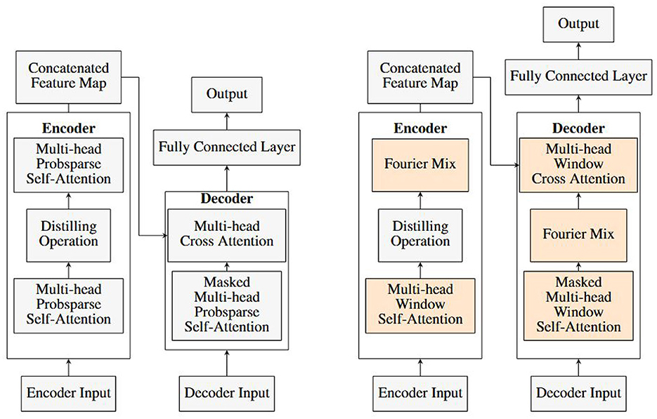
Figure 1. Model comparison: Informer (left), FWin (right, orange color denotes our contributions); FWin-S (FWin with its decoder's Fourier Mix block removed).

Table 1

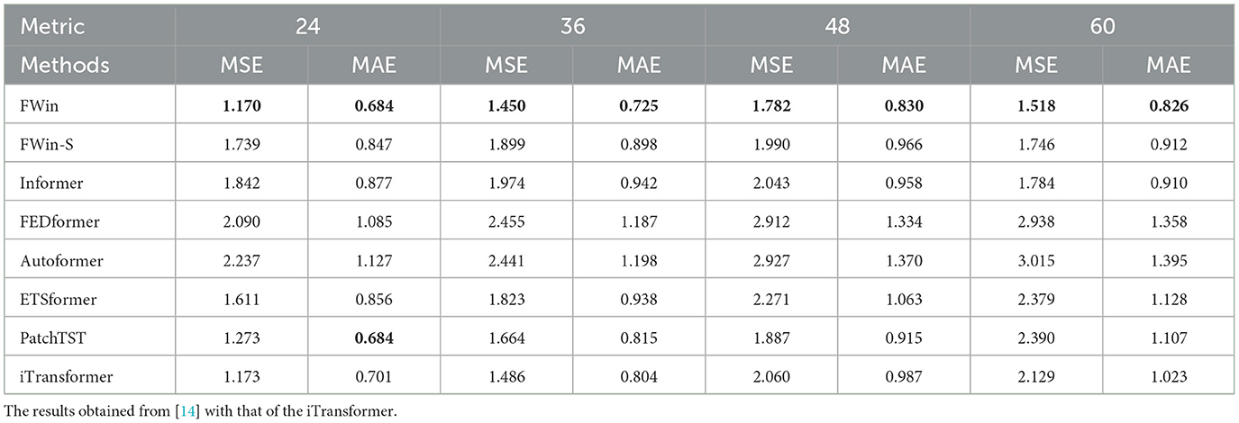
Table 1. Accuracy comparison on Singapore dengue data, best results highlighted in bold.

1.1 Organization

This paper will proceed as follows: In Section 2, we summarize the related works, provide background on full attention, window attention, Fourier mixing. In Section 3, we present FWin methodology and its complexity. In Section 4, we mathematically formulate mix window attention and prove its equivalency to canonical attention. We show that FWin is a special case of mix window attention. In Section 5, we present experimental results and analysis with ablation studies, FWin approximation in a nonlinear/non-parametric regression setting, and numerical results to verify the BDI assumption.

2 Background

2.1 Related works

Several types of attention models are related to our work here.

First, MLP mixers relax the graph similarity constraints of the self-attention and mix tokens with MLP projections. The original MLP-mixer [8] reaches similar accuracy as self-attention in vision tasks. However, such a method lacks scalability as a result of quadratic complexity of MLP projection, and suffers from parameter inefficiency for high resolution input.

Next, Fourier-based mixers apply Fourier transform to mix tokens in NLP and vision tasks. FNet [7] resembles the MLP-mixer with token mixer being the classical discrete Fourier transform (DFT), without adaptive filtering on data distribution. Global filter networks (GFNs [9]) learn filters in the Fourier domain to perform depth-wise global convolution with no channel mixing involved. Also, GFN filters lack adaptivity that could negatively impact generalization. AFNO [15] performs global convolution with dynamic filtering and channel mixing for better expressiveness and generalization. However, AFNO network parameter sizes tend to be much larger than those of the light weight vision transformer (ViT) models such as GFN-T [9], shift-window mixer Swin-T [10], and hybrid convolution-attention models MOAT-T [16], and mobile ViT [17].

For long sequence time series forecasting, the Informer [1, 11] has a hybrid convolution-attention design with a probabilistic sparsity promoting function (ProbSparse) to reduce complexity of the standard self-attention and cross-attention. We shall adopt Informer as our baseline in this work, as it compares favorably vs. efficient transformers in recent years (see Tables 1, 2 in Zhou et al. [1]). More recent improvements on benchmark data sets include Autoformer [3], FEDformer [2], and ETSformer [18], which are designed with certain prior-knowledge of datasets, e.g., using trend/seasonality decomposition and auto-correlation functions. Additionally, PatchTST [4] and iTransformer [5] focus on preserving variate information, employing independent channel processing or inverting dimensions of the multivariate inputs. However, they are not as robust on non-stationary time series as Informer (see Table 2). Informer's prediction is seen to generate spurious peaks on power grid data (3rd frame of Figure 2), while FWin predictions appear smoother and free from such distortions. Comparing Informer with full Informer in the bottom frame of Figure 2, we see that the cause of these distortions may be attributed to Probsparse. Glassoformer [13] uses group lasso penalty to enforce query sparsity and reduce complexity of full attention to speed up inference. Though this method works well on power grid data, its training time is higher than Informer since full attention is involved in network training.

Table 2

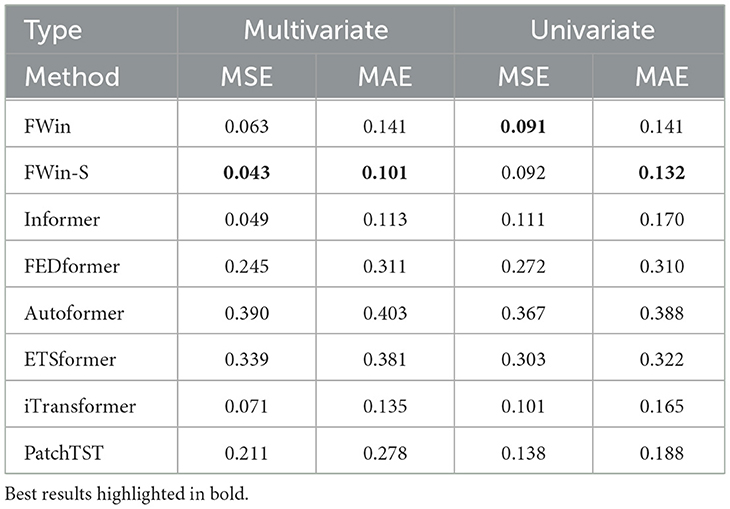
Table 2. Post-fault voltage prediction accuracy comparison on power grid dataset [12, 13] with input length of 200 and prediction of 700.

Figure 2

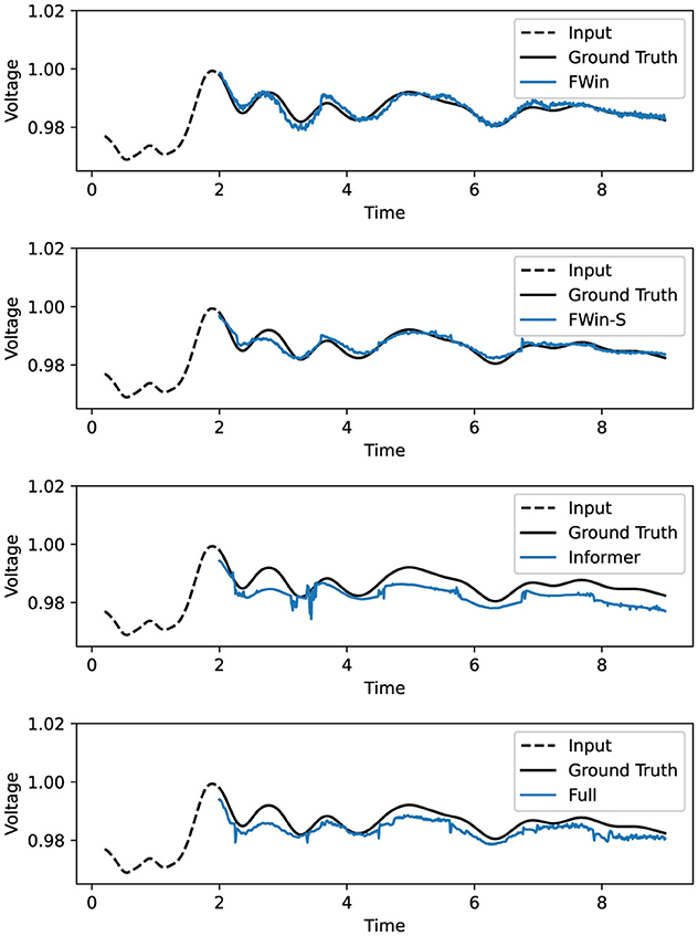
Figure 2. Univariate post fault prediction (voltage vs. time in second) on power grid data [12, 13]. FWin, FWin-S have “smooth” predictions while Informer has spurious jumps. Full in the bottom frame refers to Informer using full attention instead of probsparse. The dashed line to the left of 2 second is the input, to the right of which are the model predictions vs. the ground truth (in black).

2.2 Preliminary

2.2.1 Canonical full attention

Given an input sequence $x\in {ℝ}^{L\times d_{\mathrm{\text{model}}}}$, where L is the sequence length and d_model is the embedded dimension of the model. The input x is then converted into queries (Q), keys (K), values (V) as:

$Q=x{W}_Q+b_Q,K=x{W}_K+b_K,V=x{W}_V+b_V,$

where $W_Q,W_K,W_V\in {ℝ}^{d_{\mathrm{\text{model}}}\times d_{\mathrm{\text{attn}}}}$ are the weighted matrix, and $b_Q,b_K,b_V\in {ℝ}^{L\times d_{\mathrm{\text{attn}}}}$ are the bias matrix. In most cases, we will have d_model = d_attn, thus we will refer to d_model for the remaining of the paper.

We have

$\begin{array}{ll}Att{n}_f(Q,K,V)=\text{softmax}(Q{K}^T/\sqrt{d_{\text{model}}})V,& (1)\end{array}$

where Attn_f(·) is the attention function.

We refer to the function in Equation 1 as full attention [6], because it involves the interaction of all the key and query pairs. The final output is the weighted sum of all the values.

2.2.2 Window attention

The full attention computation involves the dot product between each query and all the keys. However, for tasks with large sequence lengths such as processing of high resolution images, the computational cost of full attention can be significant [10]. As in Swin Transformer, we divide the sequence into subsequences of smaller length, compute sub-attention for each of the subsequences individually and then concatenate all the sub-attention together. Namely, we divide sequence x into N subsequences: x⁽¹⁾, x⁽²⁾, …, x^(N), such that x = [x⁽¹⁾, x⁽²⁾, …, x^(N)]^T. Each $x^{(i)}\in {ℝ}^{L/N\times d_{\mathrm{\text{model}}}}$ for i = 1, 2, …, N, where N = L/w, w is a fixed window size. This implies we divide the queries, keys and values as follow Q = [Q⁽¹⁾, Q⁽²⁾, …, Q^(N)]^T, K = [K⁽¹⁾, K⁽²⁾, …, K^(N)]^T, V = [V⁽¹⁾, V⁽²⁾, …, V^(N)]^T. Thus we compute attention for each subsequence as follows:

$\begin{array}{ll}Att{n}_f(Q^{(i)},K^{(i)},V^{(i)})=\text{softmax}(\frac{Q^{(i)}{K}^{(i)T}}{\sqrt{d_{\text{model}}}})V^{(i)}.& (2)\end{array}$

After computing the attention for each subsequence, we concatenate the sub attentions to form the window attention:

$\begin{array}{ll}Att{n}_w(Q,K,V)=\left[\begin{array}{c}Att{n}_f(Q^{(1)},K^{(1)},V^{(1)})\\ ⋮\\ Att{n}_f(Q^{(N)},K^{(N)},V^{(N)})\end{array}\right].& (3)\end{array}$

In window attention, we compute attention on a window-by-window basis. Within each window, all the keys are multiplied with the corresponding query within that window. The output is the weighted sum of the values within the same window, rather than considering the entire set of values. This approach reduces the computational cost of computing attention on a sequence of length L from $\mathcal{O}(L^2)$ of full attention to $\mathcal{O}(Lw)$, where w is a fixed window size. Figure 3 shows the overview of full attention versus window attention.

Figure 3

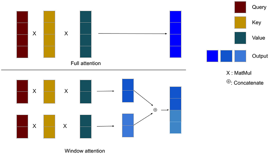
Figure 3. Overall structure of the full and window attention mechanisms. The symbol × denotes matrix multiplication between the query, key, and value matrices, while ⊕ represents the concatenation of the output matrices along the sequence dimension. In full attention, each query interacts with all of the keys and values, producing a dark blue output. In contrast, with window attention, the query interacts with only a subset of keys and values, resulting in a lighter blue output.

Window attention restricts the interaction between queries and keys by only allowing queries to attend to their local window keys. As a result, window attention provides limited or local information. On the other hand, full attention enables queries to attend to keys that are further away, allowing for global interaction. If we replace full attention with window attention, our model may lack a comprehensive understanding of global information. Therefore, it is desirable for our model to retain some level of global information when using window attention as a substitute for full attention. To incorporate global information, Swin Transformer [10] introduces shifted window attention. In this approach, before dividing the input sequence x into sub-sequences, one performs a circular shift of the indices of x by certain value. This shift allows the ending values of x to become the starting values of our input. The circular shifting process is repeated for each consecutive window attention layers.

2.2.3 FNet

Another way to promote global token interaction is by Fourier transform as proposed in FNet [7]. Given input $x\in {ℝ}^{L\times d_{\mathrm{\text{model}}}}$, one computes Fourier transform along the model dimension (d_model), then along the time dimension (L), finally taking real part to arrive at:

$\begin{array}{ll}y=\mathcal{R}({\mathcal{F}}_{\text{time}}({\mathcal{F}}_{\text{model}}(x))),& (4)\end{array}$

where $\mathcal{F}$ is 1D discrete Fourier transform (DFT), and $\mathcal{R}$ is the real part of a complex number. Here ${\mathcal{F}}_{\mathrm{\text{time}}},{\mathcal{F}}_{\mathrm{\text{model}}}$ denote the Fourier transform apply along the sequence and hidden model dimension respectively. Since DFT is free of learning parameter, one would eventually pass the transformed sequence through a Feed Forward fully-connected layer (FC). This approach can be interpreted as the Fourier transform being an effective mechanism for mixing sub-sequences (tokens) [7]. By applying the Fourier transform, the Feed Forward layer gains access to all the tokens.

3 Methodology

3.1 Informer overview

The input $x\in {ℝ}^{L\times d_{\text{data}}}$ passes through an embedding layer to encode the time scale information and return $X\in {ℝ}^{L\times d_{\mathrm{\text{model}}}}$. In the encoder, each layer consists of an attention block followed by a distilling convolution with MaxPool of stride 2 and a down-sampling to halve dimension. Thus, with 2 encoder layers, the time dimension of the first attention block is L, while the second block input is L/2. For both efficiency and causality, the decoder attention has a masked multi-head ProbSparse self-attention structure, see Figure 1 left for an overview. The ProbSparse self-attention [1] relies on a sparse query measurement function (an analytical approximation of Kullback-Leibler divergence) so that each key attends to only a few top queries for computational savings. The sparse query hypothesis or equivalently the long tail distribution of self-attention feature map is based on softmax scores in self-attention of a 4-layer canonical transformer trained on ETTh1 data set (Appendix C, [1]).

3.2 Our approach

We introduce Fourier mixed window attention (FWin) to the self-attention blocks in the encoder and decoder of Informer. Specifically, we replace the ProbSparse self-attention blocks in the encoder and decoder with window attention followed by a Fourier mixing layer. We also replace multi-head cross-attention in the decoder by a window multi-head cross-attention. Figure 1 right illustrates the key components of FWin Transformer. Different from ProbSparse attention, our FWin approach does not rely on whether the query sparse hypothesis holds on a data set.

We remark that our model differs from the FNet architecture in that Fourier transform is applied to the input along the model and the time dimensions without a subsequent Feed Forward layer. Partly this is due to the Feed Forward layer already present in the decoder of Informer before the output (Figure 1 left). We denote this specific component as Fourier Mix in our proposed FWin architecture, as depicted in Figure 1 right frame. If the Fourier Mix is removed from the decoder, we have a lighter model called FWin-S, which turns out to be a competitive design as well (see Section 5).

3.3 Encoder

Each encoder layer is defined as either a window attention layer or a Fourier Mix layer. The layers are interwoven, with the first layer being a window attention. Subsequent layers are connected by a distillation operation. For example, a 3-layer encoder will consist of a window attention layer, a distillation operation, and a Fourier Mix layer, another distillation operation, and finally another window attention layer. Figure 1 illustrates an encoder with 2 layers.

3.4 Decoder

In the decoder, a layer composed of a masked window self-attention followed by a Fourier Mix and then window cross attention with layer normalization in between. Toward the end of the layer, convolutions and layer normalization are applied. Figure 1 shows a decoder with one layer.

3.5 Window cross attention

In a self-attention layer, the query and key vectors have the same time dimension, allowing us to use the same window size to split these vectors. However, in the case of cross attention, this may not hold true, especially if the encoder includes dimension reduction layers. In such cases, the key and value vectors may have a smaller time dimension compared to the query vectors, which originate from the decoder. Additionally, the encoder and decoder inputs may have different input time dimensions, as is the case in our specific problem. To ensure equal number of attention windows in cross attention, we divide the query, key, and value vectors based on the number of windows rather than the window size. This adjustment accounts for varying time dimensions and guarantees a consistent number of attention windows for the cross attention operation.

3.6 Complexity

With the replacements in the attention computation, our approach offers significant complexity reduction compared to Informer. In the encoder, the first attention layer partitions the time dimension of the input by a window of size w, by default w = 24, resulting in each window attention input having dimensions of w × d_model. Thus the cost of this layer is $\mathcal{O}(Lw{d}_{\mathrm{\text{model}}})$. Furthermore, in the second attention layer, the computation of attention is completely replaced by the Fourier Mix layer, eliminating three linear projections for query, key, and value vectors. Since we apply the FFT over the time dimension and the model dimension, the total cost for the Fourier Mix layer is $\mathcal{O}(L{d}_{\text{model}}\log (L{d}_{\text{model}}))$. Overall Informer has complexity of $\mathcal{O}(L\log (L)d_{\text{model}}+L\log (L)d_{\text{model}}+L\log (L)d_{\text{model}}+L^2{d}_{\text{model}})$ and FWin is $\mathcal{O}(Lw{d}_{\text{model}}+L{d}_{\text{model}}\log (L{d}_{\text{model}})$ +Lwd_model + Ld_model log(Ld_model) +Lwd_model). The $L^2{d}_{\mathrm{\text{model}}}$ cost of Informer comes from full cross attention in its decoder (Figure 1 left). In FWin, this cost is reduced to Lwd_model by window cross attention (Figure 1 right).

4 Theoretical results

In this section, we will present the mathematical justification for our approach. The goal is to demonstrate mixing tokens among the windows attention is a good approximator of full attention. We begin with preliminary definitions.

Definition 4.1. Let A ∈ ℝ^{L × L}, with the (i, j)-th entry of A denoted by a_ij. Let w ∈ ℕ be a factor of L. For every n ∈ {1, …, L/w}, let A_n be the sub-matrix of A such that the entries of A_n are composed of ${(a_{ij})}_{i=w(n-1)+1,j=w(n-1)+1}^{i=nw,j=nw}$. We say A is block diagonally invertible (BDI) if for every n, A_n is invertible.

Definition 4.2. Let Q, K ∈ ℝ^{L × d} be the query, key matrix respectively. Define the attention matrix as:

$\begin{array}{ll}Attn(Q,K):=\text{softmax}(Q{K}^T/\sqrt{d}).& (5)\end{array}$

Definition 4.3. Let Q, K, V ∈ ℝ^{L × d} be the query, key matrix respectively. Define the full attention as:

$\begin{array}{ll}Att{n}_f(Q,K,V):=\text{softmax}(Q{K}^T/\sqrt{d})V=Attn(Q,K)V.& (6)\end{array}$

Definition 4.4. Let Q, K, V ∈ ℝ^{L × d} be the query, key, value matrix respectively with q_i, k_i, v_i the i-th row of the matrix Q, K, V. Let w ∈ ℕ be the window size, such that w divides L. Define the window attention as:

$\begin{array}{ll}Att{n}_w(Q,K,V,w):=\left[\begin{array}{c}{\displaystyle {\sum }_{j\in J(1)}\frac{\exp (q_1{k}_j^T/\sqrt{d})v_j}{{\gamma }_1}}\\ ⋮\\ {\displaystyle {\sum }_{j\in J(L)}\frac{\exp (q_L{k}_j^T/\sqrt{d})v_j}{{\gamma }_L}}\end{array}\right].& (7)\end{array}$

Here J(m) = {Mw + 1, …, (M + 1)w}, where $M=\lfloor \frac{m-1}{w}\rfloor$. And

$\begin{array}{ll}{\gamma }_m={\displaystyle \sum _{j\in J(m)}}exp(q_m{k}_j^T/\sqrt{d}).& (8)\end{array}$

Definition 4.5. Let A ∈ ℝ^{L × L} and Q, K, V, w be the same as defined in Definition 4.4, define the mixed window attention as:

$\begin{array}{ll}Att{n}_{mw}(Q,K,V,w,A):=AAtt{n}_w(Q,K,V,w).& (9)\end{array}$

Theorem 4.6. Let Q, K, V ∈ ℝ^{L × d}. Let w ∈ ℕ such that w divides L. If Attn(Q, K) is BDI, then there exists a matrix A ∈ ℝ^{L × L} such that

$\begin{array}{ll}Att{n}_f(Q,K,V)=Att{n}_{mw}(Q,K,V,w,A).& (10)\end{array}$

In particular, we can construct the exact value of A.

Proof. We have the i-th row of full attention is

$\begin{array}{ll}Att{n}_f^i={\displaystyle \sum _{j=1}^L}\frac{exp(q_i^T{k}_j/\sqrt{d})v_j}{{\beta }_i},& (11)\end{array}$

where ${\beta }_i=\sum _{j=1}^{L}exp(q_i{k}_j^T/\sqrt{d})$. Let α_im be the i, m entry of A, the i-th row of mixed window attention is

$\begin{array}{ll}Att{n}_{mw}^i={\displaystyle \sum _{m=1}^L}{\alpha }_{im}{\displaystyle \sum _{j=Mw+1}^{(M+1)w}}\frac{exp(q_m^T{k}_j/\sqrt{d})v_j}{{\gamma }_m},& (12)\end{array}$

where ${\gamma }_m=\sum _{j\in J(m)}exp(q_m{k}_j^T/\sqrt{d})$, with J(m) = {Mw + 1, …, (M + 1)w}, where $M=\lfloor \frac{m-1}{w}\rfloor$.

Consider the following cases:

• If i = m and j ∈ {Mw + 1, …, (M + 1)w}, set $\frac{1}{{\beta }_i}=\frac{{\alpha }_{ii}}{{\gamma }_m}$.

• If i ≠ m and j ∈ {Mw + 1, …, (M + 1)w} and j ∈ {Iw + 1, …, (I + 1)w}, where $I=\lfloor \frac{i-1}{w}\rfloor$, set α_im = 0.

• If i ≠ m and j ∈ {Mw + 1, …, (M + 1)w} and j ∉ {Iw + 1, …, (I + 1)w}, where $I=\lfloor \frac{i-1}{w}\rfloor$. For each j we set

$\begin{array}{ll}\frac{exp(q_i{k}_j^T/\sqrt{d})}{{\beta }_i}={\displaystyle \sum _{m\in J(j)}}\frac{{\alpha }_{im}exp(q_m{k}_j^T/\sqrt{d})}{{\gamma }_m}.& (13)\end{array}$

For each i and set of {m, j} pairs, we have to solve a system of w equations and unknowns. We now invoke the BDI assumption of Attn(Q, K) to show that this system of equations has unique solution. Let C be the coefficient matrix of the right hand side of the system of equations in Equation 13. We observe that C^T is invertible, because each row of C^T is a scaled version of a square sub matrix along the diagonal of Attn(Q, K), and each square sub-matrix along the diagonal of Attn(Q, K) is invertible. The invertibility of C then follows from that of C^T.

We completed the construction of A as claimed in the theorem.

Remark 4.7. The BDI assumption in Theorem 4.6 is a sufficient condition and not a necessary condition. We only need BDI to solve the system of Equation 13 in the proof. This may be solvable even if BDI is not met. In this case, the solution will not be unique. In particular, the theorem holds true under no assumption when window size is 1. In Table 3, we showed that window size of 1 has competitive performance compare to others. In Section 5.5, we will show in practice that BDI is satisfied by most of the datasets presented in this paper.

Table 3

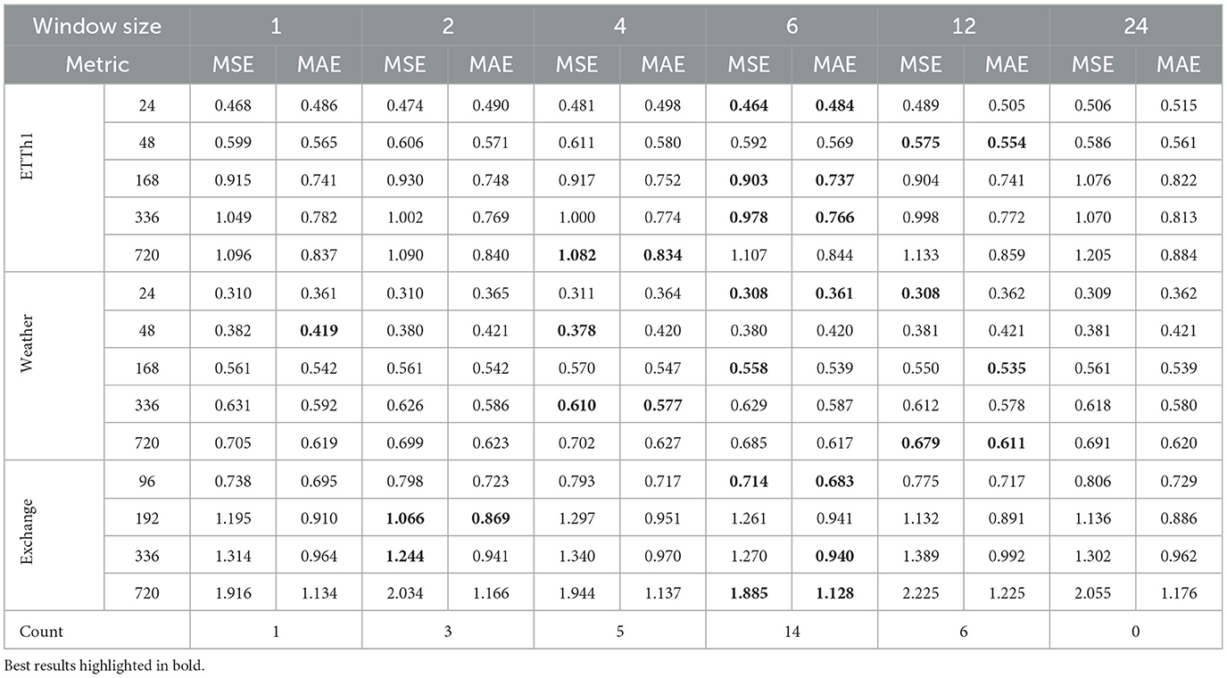
Table 3. Accuracy comparison of FWin model using different window sizes for various datasets on the multivariate task.

A drawback of directly learn a mixing matrix is the computational cost of matrix multiplication in which we want to alleviate from full attention. Fourier transformation can be utilized as a mixing matrix with a lower cost. We will show that this is sufficient.

Definition 4.8. Let A ∈ ℝ^{L × L} and Q, K, V, w be the same as defined in Definition 4.4, define the Fourier-mixed window attention as:

$\begin{array}{ll}Att{n}_{Fwin}(Q,K,V,w,A):=A\mathcal{F}(Att{n}_w(Q,K,V,w)),& (14)\end{array}$

where $\mathcal{F}$ is the discrete Fourier transform.

Corollary 4.9. Let Q, K, V and w be the same as defined in Theorem 4.6. If Attn(Q, K) is BDI, then there exists a matrix A ∈ ℂ^{L × L} such that

$\begin{array}{ll}{\text{Attn}}_f(Q,K,V)={\text{Attn}}_{Fwin}(Q,K,V,w,A).& (15)\end{array}$

Proof. From Theorem 4.6, there exists B ∈ ℝ^{L × L} such that

$\begin{array}{ll}Att{n}_f(Q,K,V)=Att{n}_{mw}(Q,K,V,w,B).& (16)\end{array}$

Thus if we let $A=B{\mathcal{F}}^{-1}$, then we are done.

Definition 4.10. Let A ∈ ℝ^{L × L} and Q, K, V, w be the same as defined in Definition 4.4, define the Hartley-mixed window attention as:

$\begin{array}{ll}{\text{Attn}}_{Hwin}(Q,K,V,w,A):=A\mathcal{H}(Att{n}_w(Q,K,V,w)),& (17)\end{array}$

where $\mathcal{H}$ is the Hartley transform [19].

Corollary 4.11. Let Q, K, V, and w be the same as defined in Theorem 4.6. If Attn(Q, K) is BDI, then there exists a matrix A ∈ ℝ^{L × L} such that

$\begin{array}{ll}{\text{Attn}}_f(Q,K,V)={\text{Attn}}_{Hwin}(Q,K,V,w,A).& (18)\end{array}$

Proof. From Theorem 4.6, there exists B ∈ ℝ^{L × L} such that

$\begin{array}{ll}Att{n}_f(Q,K,V)=Att{n}_{mw}(Q,K,V,w,B).& (19)\end{array}$

Thus if we let $A=B{\mathcal{H}}^{-1}$, then we are done.

Per usual in neural networks, the query, key, and value matrices are linear projection of an input x, which could be randomly drawn from some distribution. We will show under certain stochastic conditions, Theorem 4.6 holds. We will begin with the definition of the sufficient condition.

Definition 4.12. Let $X_1,\dots ,X_{L^2}$ be random variables. The random variables are jointly absolutely continuous if the random vector $X=(X_1,\dots ,X_{L^2})$ has a jointly absolutely continuous distribution, that is there exists integrable function f : ℝ^L2 → ℝ such that

$\begin{array}{ll}\mathbb{P}\left\{X\in B\right\}={\displaystyle {\int }_B}f(x)dx,\forall B\in B^{L^2}.& (20)\end{array}$

Here 𝔹^L2 is the L² dimensional Borel set.

We know that suppose the joint distribution of the entries of a matrix A is absolutely continuous, then A is invertible with probability 1. This is because the non-invertible matrices form a low dimensional manifold M in ℝ^L2. The probability of A being non-invertible is the probability that A is in M. This equals to the integral of some density function f : ℝ^L2 → ℝ over M, which equals to zero since dimension of M is less than L².

Corollary 4.13. Let Q, K, V be ℝ^{L × d} random matrices, and w is a factor of L. If the entries of Attn(Q, K) is jointly absolutely continuous, then with probability 1, there exists a matrix A ∈ ℝ^{L × L} such that

$\begin{array}{ll}Att{n}_f(Q,K,V)=Att{n}_{mw}(Q,K,V,w,A)& (21)\end{array}$

Proof. It is clear that if Attn(Q, K) is jointly absolutely continuous, then any marginal distributions is jointly absolutely continuous. Thus it follows that Attn(Q, K) satisfies BDI property with probability 1. Hence, the corollary follows from Theorem 4.6.

5 Experiments

5.1 Experimental data and details

The default setup of the model parameters is shown in Table 4. For Informer, we used their up to date code,¹ which incorporated all the functionalities described recently in Zhou et al. [11]. In our experiments, we average over 5 runs. The total number of epochs is 6 with early stopping. We optimized the model with Adam optimizer, and the learning rate starts at 1e⁻⁴, decaying two times smaller every epoch. For fair comparison, all of the hyper-parameters are the same across all the models which were trained/tested on a desktop machine with four Nvidia GeForce 8G GPUs.

Table 4

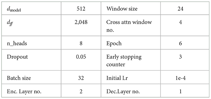
Table 4. Model default parameters.

5.1.1 Benchmark datasets

Details of public benchmark datasets used in the main paper are described below:

ETT (Electricity Transformer Temperature)²: The dataset contains information of six power load features and target value “oil temperature.” We used 2 h datasets ETTh₁ and ETTh₂, and the minute level dataset ETTm₁. The train/val/test split ratio is 6:2:2.

Weather (Local Climatological Data)³: The dataset contains local climatological data collected hourly in 1,600 U.S. locations over 4 years from 2010 to 2013. The data consists of 11 climate features and target value “wet bulb.” The train/val/test split ratio is 7:1:2.

ECL (Electricity Consuming Load)⁴: This dataset contains electricity consumption (Kwh) of 321 clients. The data convert into hourly consumption of 2 year and “MT_320” is the target value. The train/val/test split ratio is 7:1:2.

Exchange⁵ [20]: The dataset contains daily exchange rates of eight different countries from 1990 to 2016. The train/val/test split ratio is 7:1:2.

ILI⁶: The dataset contains weekly recorded influenza-like illness (ILI) patients data from Centers for Disease Control and Prevention of the United States from 2002 to 2021. This describes the ratio of patients seen with ILI and the total number of the patients. The train/val/test split ratio is 7:1:2.

5.1.2 Additional non-stationary data

In addition to the benchmark datasets, we also validate our model on non-stationary datasets.

Power grid: Simulated New York/New England 16-generator 68-bus power system [12, 13]. The system has 88 lines linking the buses, and can be regarded as a graph with 68 nodes and 88 edges. The dataset has over 2,000 fault events, where each event has signals of 10 second duration. These signals contain voltage and frequency from every bus, and current from every line. The train/val/test split is 1,000:350:750.

Dengue [14]: The dataset contains 1,000 weeks of Singapore's weekly dengue data spanning from 2000 to 2019. Dataset includes the climate and oceanic anomaly features. The train/val/test split ratio is 6:2:2.

5.2 Setup of experiments

For all the experiments to compute the errors, the encoder's input sequence and the decoder's start token are chosen from {24, 48, 96, 168, 336, 720} for the ETTh₁, ETTh₂, Weather and ECL dataset, and from {24, 48, 96, 192, 288, 672} for the ETTm dataset. The default window size is 24. We use a window size of 12 when the encoder's input sequence is 24. For the Exchange, ILI, and Traffic datasets, we use the same hyper-parameters as those provided in Autoformer. The encoder's input sequence is 96 and decoder's input sequence is 48. The window size is 24 for Exchange and Traffic. For ILI, we use an input length of 36 for the encoder and 18 for decoder, with window size of 6. The number of windows on the cross attention is set to 3. The models are trained for 6 epochs with learning rate adjusted by a factor of 0.5 every epoch.

For the power grid dataset [12, 13], the encoder and decoder inputs are set to 200. The prediction length is 700, and the window size is 25. The models are trained for 80 epochs with an early stopping counter of 30. The learning rate is adjusted every 10 epochs by a factor of 0.85. For the dengue dataset, we use the same hyper-parameters as in ILI dataset, because of its size and type.

5.3 Results and analysis

5.3.1 Benchmarks

We present a summary of the univariate and multivariate evaluation results for all methods on 7 benchmark datasets in Tables 5, 6. MAE $=\frac{1}{n}\sum _{i=1}^n|y-\widehat{y}|$ and MSE $=\frac{1}{n}\sum _{i=1}^n{(y-\widehat{y})}^2$ are used as evaluation metrics. The best results are highlighted in boldface, and the total count at the bottom of the tables indicates how many times a particular method outperforms others per dataset.

Table 5

Table 5. Accuracy comparison on LSTF benchmark univariate data, best results highlighted in bold.

Table 6

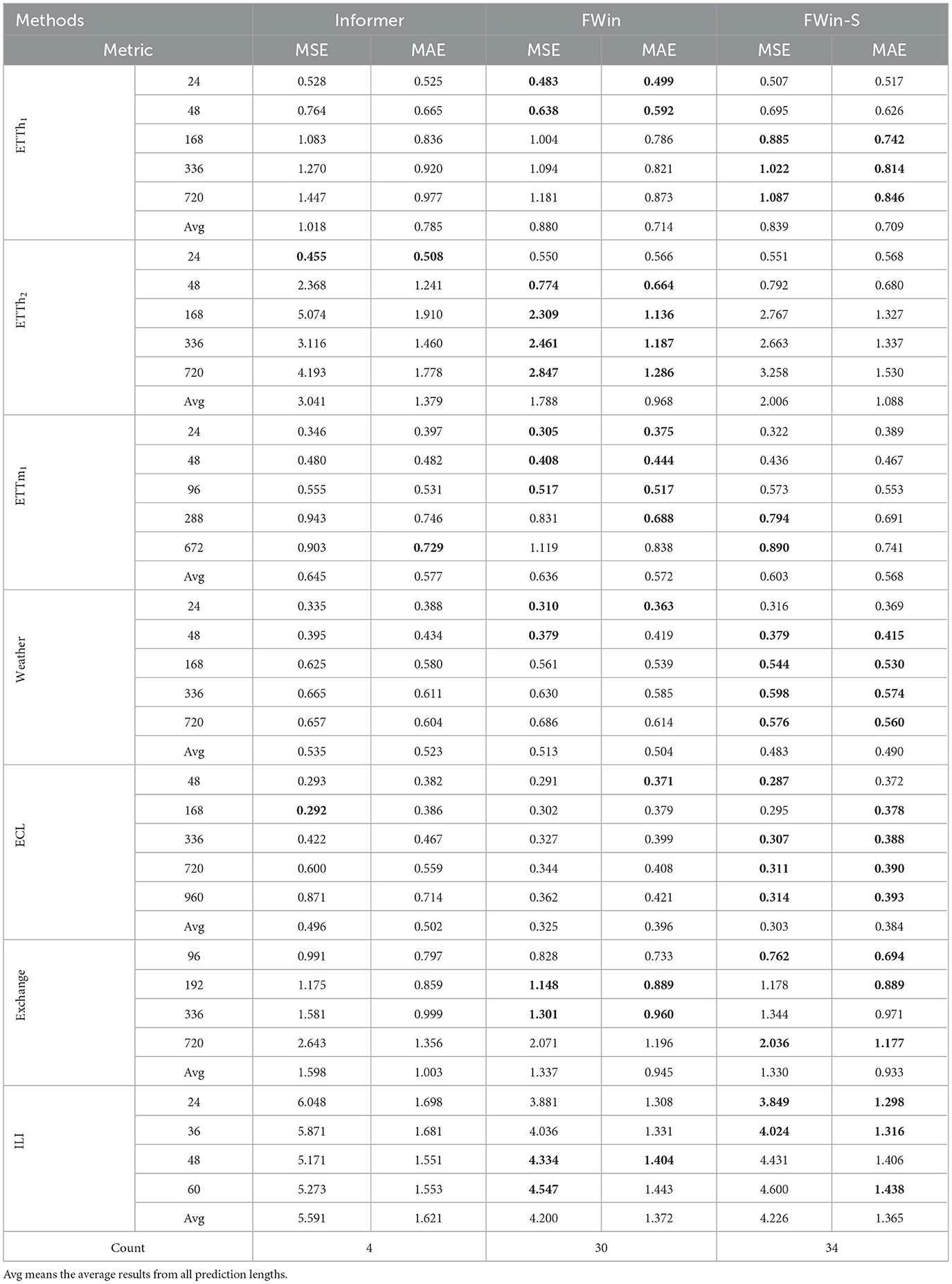
Table 6. Accuracy comparison on LSTF benchmark multivariate data, best results highlighted in bold.

For the univariate setting, each method produces predictions for a single output over the time series. From Table 5, we observe the following:

(1) FWin and FWin-S achieve comparable performance.

(2) When comparing FWin and Informer, FWin outperforms the Informer by a margin of 50 to 16.

(3) FWin performs well on the ETT, Exchange, ILI datasets, it remains competitive for the Weather dataset. However, it performs not as well on the ECL dataset. This could be due to the differences caused by the dataset, which is common in time-series model [21], or Informer's ProbSparse hypothesis satisfied well for this dataset.

(4) The average MSE reduction is 19.60%, and MAE is about 11.88%, when comparing FWin with Informer.

For the multivariate setting, each method produces predictions based on multiple features over the time series. From Table 6, we observe that:

(1) The light model FWin-S leads the count at 34 total, followed closely by FWin with a total count of 30.

(2) In a head to head comparison, FWin outperforms Informer by a large margin (59 to 7).

(3) Though FWin and FWin-S have close accuracies in itemized-metric comparison on the benchmarks, FWin is overall more robust (e.g., it behaves better on non-stationary dengue disease dataset, see Table 1 and Section 5.3.3).

(4) The average MSE (MAE) reduction from Informer to FWin is about 16.33% (10.96%).

5.3.2 Power grid

Informer's prediction accuracies on the benchmark datasets in Tables 5, 6 have been largely improved by recent transformers such as iTransformer [5], PatchTST [4] designed to prioritize variate information; and Autoformer [3], FEDformer [2], and ETSformer [18] designed with certain prior-knowledge of datasets, e.g., using auto-correlation or trend/seasonality decomposition. Like Informer, FWin has no prior-knowledge based operation, which helps to generalize better on non-stationary time series where seasonality is absent. Such a situation arises in post-fault decision making on a power grid where predicting transient trajectories is important for system operators to take appropriate actions [22], e.g., a load shedding upon a voltage or frequency violation. We carry out experiments on a simulated New York/New England 16-generator 68-bus power system [12, 13]. Table 2 shows that FWin and FWin-S improve or maintain Informer's accuracy in a robust fashion while the five recent transformers pale in comparison. Figure 4 illustrates model predictions on the power grid dataset [12, 13]. FWin and Informer outperform FEDformer, Autoformer, iTransformer, and PatchTST.

Figure 4

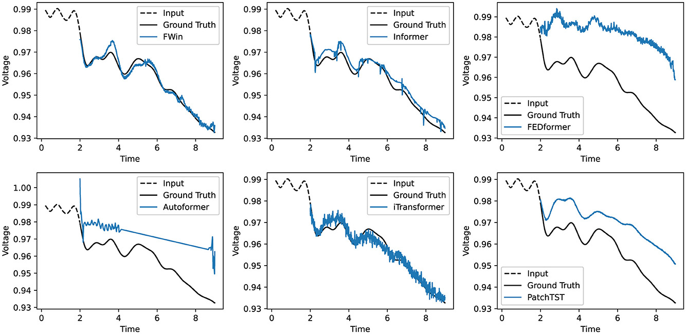
Figure 4. Multivariate post fault prediction comparison (voltage vs. time in second) on power grid data [12, 13]: {FWin,Informer} outperform (FED, Auto, iTrans)formers and PatchTST. The dashed line under 2 second duration is the input, to the right of which are the predictions vs. the ground truth (in black).

5.3.3 Singapore dengue

In Tran et al. [14], FWin transformer is successfully applied on the dataset to study dengue disease prediction under the influence of climate and ocean factors. In this multi-variate to uni-variate prediction task, the goal is to predict the number of dengue cases given multiple environmental features such as climate, ocean, humidity and temperature. FWin performs better than Informer, FEDformer, Autformer, ETSformer, and PatchTST. Extending this work, we added the result of iTransformer on this Singapore dengue dataset and compare all the above networks in Table 1. The result shows that FWin and iTransformer are comparable on short prediction length of 24 and 36, however FWin is better than iTransformer on prediction length of 48 and 60.

5.3.4 Speed up

Besides performance and robustness, the inference and training times of the models (in particular the former) are also of our interest and are summarized below:

(1) Compared to Informer, FWin achieves average speed up factors of 1.7 and 1.4 for inference and training times respectively (see Table 7). The ILI dataset has the lowest speed-up factor because both the input and the prediction lengths are small.

(2) FWin's inference and training times are very close to those of FWin-S. This indicates that the Fourier Mix layer in the decoder adds a minimal overhead to the overall model. The FWin-S model exhibits the fastest inference and training times, as expected because it is the model with smallest parameter size here.

(3) FWin has approximately 8.1 million parameters, whereas Informer has around 11.3 million parameters under default settings, resulting in a reduction about 28%. On the ETTh1 prediction length task of 720, Informer has 5.85 GFLOPs, while FWin has 5.32 GFLOPs under identical setting. This confirms our analysis that Informer's cross attention is full attention, whereas FWin's windowed cross attention is much more efficient.

(4) The inference time for Informer increases with prediction length. FWin's inference time exhibits minimal growth. The Exchange dataset demonstrates this effect as we used the same input length for all prediction lengths, and ran the models on a single GPU (see Supplementary material).

(5) FWin's inference time is about 1.6 to 6 times faster compared to ETSformer, FEDformer, and Autoformer (see Table 8).

Table 7

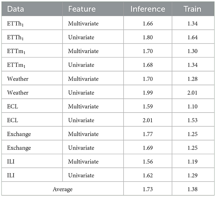
Table 7. Average inference/training speed-up factors of FWin vs. Informer.

Table 8

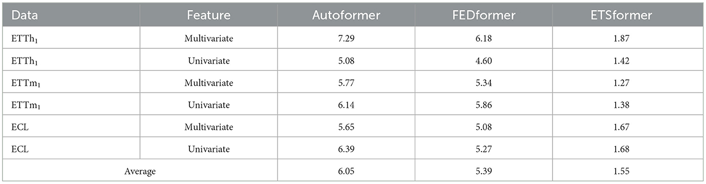
Table 8. Average inference speed-up factors of FWin vs. SOTAs.

5.4 Ablation studies

5.4.1 Benefits of combining fourier and window attention

We examined the benefits of combining window attention and Fourier mixing by experiments on the ETTh1 and Weather dataset. Table 9 shows that Fourier-mixed window attention outperforms using Fourier mixing alone (FNet [7]) in accuracy. In addition, it also suggests that Fourier-mixed window attention is better overall than shifted window attentions in the encoder. In view of Tables 5, 6, FWin-S is better than Swin on metric 720 in MSE (comparable in MAE).

Table 9

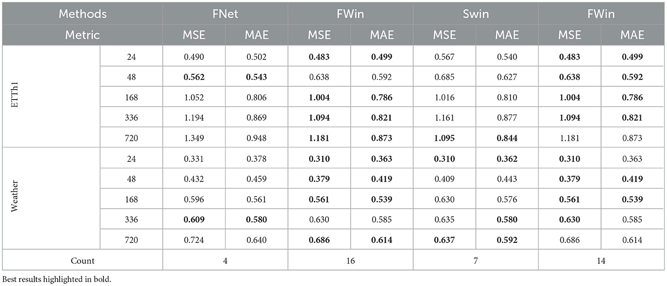
Table 9. FWin vs. FNet [7] (replacing ProbSparse attention of Informer by Fourier-Mix followed by an FC layer) and FWin vs. Swin [10] (replacing Fourier Mix in FWin by a shifted window attention) on multivariate data.

5.4.2 Effect of window size parameter

Window size is an important parameter for FWin. In this section we will explore the effect of window size to model performance across many datasets presented in the paper. We present the results in Table 3. We observe that across the datasets, window size of 6 provides the best results overall. Window size of 1 provides competitive results compare to the best window size of 6. In general, under various window sizes, the performance is consistent. Optimizing the window size for each data set may increase performance of our model. However, to keep the experiments consistent, we decide to keep the window size at a fixed constant 24. The time scale of a dataset may impact the choice of window size. Many of the datasets have hourly time scale, thus choosing a window size of 24 is meaningful in covering a daily observation. The flexible choice of window size enables the practical application of the method to various datasets with well-known temporal dependencies, such as the lag patterns in the dengue dataset.

5.4.3 FWin and non-parametric regression

The full self-attention function [6] can be conceptualized as an estimator in a non-parametric kernel regression problem in statistics [23]. Let the key vectors serve as the training inputs and the value vectors as the training targets. The key-value pairs {k_j, v_j} for j = 1, …, N, come from the model

$\begin{array}{ll}{v}_j=f(k_j)+{ϵ}_j,& (22)\end{array}$

where f is an unknown function to be estimated and ϵ_j are zero mean independent noisy perturbations. Let the key vectors k₁, k₂, …, k_N be i.i.d. samples from a distribution function p(k), and the key-value pairs (v₁, k₁), …, (v_N, k_N) be i.i.d. samples from the joint density p(k, v). Since 𝔼[v_j|k_j] = f(k_j), the classical Nadaraya-Watson method [24–26] approximates p by a sum of Gaussian kernels and gives the estimate of f below:

$\begin{array}{ll}{\widehat{f}}_{\sigma }(k):={\displaystyle \sum _{j=1}^N}\frac{v_j{\varphi }_{\sigma }(k-k_j)}{{\displaystyle {\sum }_{j=1}^N}{\varphi }_{\sigma }(k-k_j)},& (23)\end{array}$

where ϕ_σ(·) is the isotropic multivariate Gaussian density function with diagonal covariance matrix ${\sigma }^2{\text{I}}_D$. In particular if k = q_i, and the k_j's are normalized, one obtains ${\widehat{f}}_{\sigma }(q_i)=$

$\begin{array}{ll}\frac{{\displaystyle {\sum }_{j=1}^N{v}_j\exp (q_i{k}_j^T/{\sigma }^2)}}{{\displaystyle {\sum }_{j=1}^N\exp (q_i{k}_j^T/{\sigma }^2)}}={\displaystyle \sum _{j=1}^N\text{softmax}}(q_i{k}_j^T/{\sigma }^2)v_j.& (24)\end{array}$

Letting ${\sigma }^2=\sqrt{d_{\mathrm{\text{model}}}}$, where d_model is the dimension of q_i (k_j), turns estimator (Equation 24) into the softmax self-attention (Equation 1).

To build a window attention, we allow the query vector q_i to interact only with nearby key and value vectors. Thus the window version of the softmax estimator is ${\bar{f}}_{\sigma }(q_i):=$

$\frac{{\displaystyle {\sum }_{j\in J(i)}{v}_j\exp (q_i{k}_j^T/{\sigma }^2)}}{{\displaystyle {\sum }_{j\in J(i)}\exp (q_i{k}_j^T/{\sigma }^2)}}={\displaystyle \sum _{j\in J(i)}\text{softmax}}(q_i{k}_j^T/{\sigma }^2)v_j$

where J(i) is the index set that corresponds to the set of keys the query q_i interact with. In view of the fully connected (MLP) layer after the Fourier mixing layer and before the output in Figure 1, we define the analogous FWin estimator for the regression model as

$\begin{array}{ll}{\tilde{f}}_{\sigma }(q_i):=A·\mathcal{R}(\mathcal{F}({\bar{f}}_{\sigma }(q_i))),& (25)\end{array}$

where $\mathcal{R}$ takes the real part, $\mathcal{F}$ is the discrete Fourier transform, · represents matrix multiplication, and A is a real matrix to be learned from the training data by minimizing the sum of squares error (MSE) of the regression model (Equation 22).

5.4.3.1 Kernel regression experiment

To examine the differences among the three estimators $\widehat{f}$, $\bar{f}$, and $\tilde{f}$, we opt for the Laplace distribution function f = exp(−α|x|), for α = 0.01, as the ground truth nonlinear function acting componentwise on the input to the regression model (Equation 22). We use a set of query, key, value vectors from Informer^† [1] on ETTh₁ multivariate data set with prediction length (metric) of 720. We choose this particular data set because Informer^† [1] with full softmax self-attention has the best performance there. The key vectors may not satisfy the theoretical i.i.d. assumption [23]. In this experiment, we have a set of 168 query and key vectors from each of the 8 heads. Denote query q_i, and key k_j vectors for i, j = 1, 2, …, 168. The value vectors are v_j = f(k_j). We divide the data into 136 vectors for training and the remaining 32 for testing. The mean square error (MSE) in testing of the estimator $\widehat{f}(q_{i_n})$ for n = 1, 2, …, 32, are labeled full estimator in Figure 5. Similarly, we compute MSEs for ${\bar{f}}_{\sigma }(q_{i_n})$, and $\tilde{f}(q_{i_n})$, using window size of 4, where A is learned by solving a least squares problem. Figure 5 compares the MSE of the three estimators over data from 8 heads. We observe that the FWin estimator consistently outperforms the window attention estimator, and approaches the full softmax attention. In heads 0/1/4, FWin outperforms the full softmax attention estimator which is not theoretically optimal for the regression task [23]. In conclusion, the regression experiment on the three estimators indicates that FWin is a simple and reliable local-global attention structure with competitive capability, lending added support to its robust performance.

Figure 5

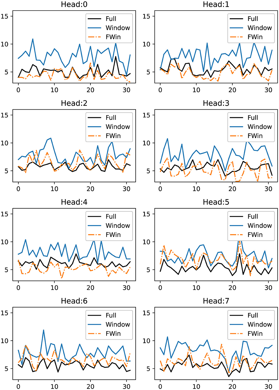
Figure 5. MSE error vs. query number comparison of full softmax attention (black), window attention (blue) and FWin attention (orange) in the non-parametric regression model (Equation 22) based on key vectors of a full attention layer of Informer^† [1] trained from the ETTh₁ data set.

5.5 Condition number of attention matrix

Theorem 4.6 requires the attention matrix to be BDI. In this section, we verify that in practice BDI is satisfied by many of the datasets here. The experimental set-up is:

• Run simulations on the Informer model using full attention instead of Probsparse.

• Collect the full attention matrix of the first encoder block of the Informer.

• Given a window size w, compute the condition numbers of w × w sub-matrices along the diagonal of the attention matrix.

• If the condition numbers are finite, then BDI is true and this instance is collected for a histogram plot, otherwise it is counted as a failure.

Using the procedure above, we plot all condition numbers for all simulations of the ETTh₁, Weather, and ILI dataset. For all the simulations, we use the same hyper-parameters as in the experiment sections. Due to memory space constraint, we report the first 11 batches of the test datasets.

From Figure 6, we observe that ETTh1, Weather, ILI datasets satisfy the assumption of the theorem relatively well. In particular, ETTh1 has a few infinite condition number out of millions. For ILI, approximately 0.4–0.5% of the condition numbers are infinite, while the Weather dataset has around 3% infinite condition numbers. We also noted that the condition numbers increase with the window size for WTH dataset. We selected these three datasets to demonstrate the robustness of the assumption, as they span different temporal granularities from minutes in WTH, to hours in ETTh1, and weeks in ILI. Combining this observation with the results from Table 3, we suggest using a small window size, as it maintains competitive performance compared to larger window sizes while ensuring that the BDI condition is satisfied in practice.

Figure 6

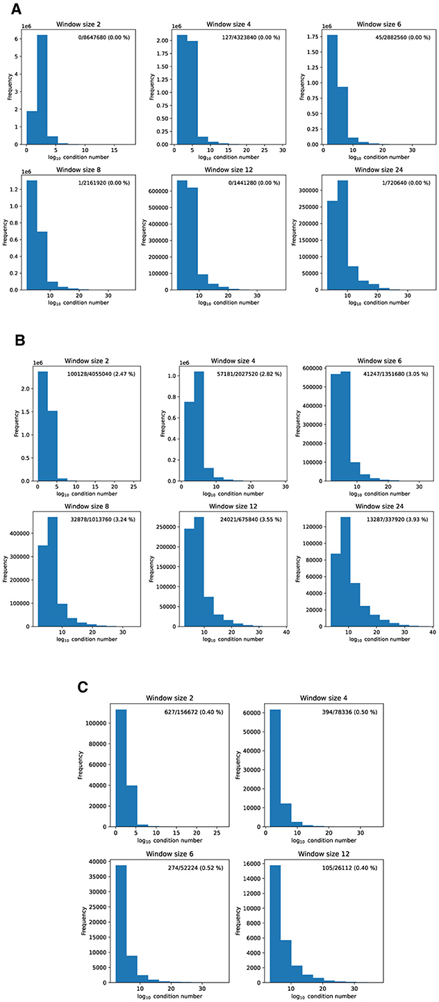
Figure 6. Condition numbers under various window sizes for different datasets. On the top right corner of each subplot there is a label “n/m (k %)” on the top right, it denotes the number of infinite condition numbers (n) over the total condition numbers (m), with a percentage (k). (A) ETTh1. (B) WTH. (C) ILI.

6 Conclusion

We introduced FWin Transformer and its light weight version FWin-S to successfully reduce the complexity, and improve/maintain the accuracy of Informer by replacing its ProbSparse and full attention layers with window attention and Fourier mixing blocks in both encoder and decoder. The FWin attention approach does not rely on sparse attention hypothesis or periodic like patterns in the data, hence also achieves robustness especially on highly non-stationary data. The experiments on uni/multi-variate datasets and theoretical guarantees demonstrated FWin's merit in fast and reliable inference on LSTF tasks.

In future work, we plan to (1) embed FWin in an encoder only architecture (e.g., iTransformer [5]) for acceleration and improved generalization; (2) optimize the FWin approach toward accurate, robust and fast transformers in challenging non-stationary real-world LSTF applications.

Data availability statement

The original contributions presented in the study are included in the article/Supplementary material, further inquiries can be directed to the corresponding author.

Author contributions

NT: Software, Investigation, Writing – review & editing, Visualization, Writing – original draft, Data curation, Formal analysis. JX: Funding acquisition, Methodology, Writing – review & editing, Resources, Conceptualization.

Funding

The author(s) declare that financial support was received for the research and/or publication of this article. This work was partially supported by the NSF grants DMS-1952644, DMS-2151235, DMS-2219904, and a Qualcomm Faculty Award.

Acknowledgments

This manuscript has been released as a pre-print at https://arxiv.org/abs/2307.00493 [27].

Conflict of interest

The authors declare that the research was conducted in the absence of any commercial or financial relationships that could be construed as a potential conflict of interest.

Generative AI statement

The author(s) declare that no Gen AI was used in the creation of this manuscript.

Publisher's note

All claims expressed in this article are solely those of the authors and do not necessarily represent those of their affiliated organizations, or those of the publisher, the editors and the reviewers. Any product that may be evaluated in this article, or claim that may be made by its manufacturer, is not guaranteed or endorsed by the publisher.

Supplementary material

The Supplementary Material for this article can be found online at: https://www.frontiersin.org/articles/10.3389/fams.2025.1600136/full#supplementary-material

Footnotes

1. ^https://github.com/zhouhaoyi/Informer2020

2. ^https://github.com/zhouhaoyi/ETDataset

3. ^https://www.ncei.noaa.gov/data/local-climatological-data

4. ^https://archive.ics.uci.edu/ml/datasets/ElectricityLoadDiagrams20112014

5. ^https://github.com/laiguokun/multivariate-time-series-data

6. ^https://gis.cdc.gov/grasp/fluview/fluportaldashboard.html

References

1. Zhou H, Zhang S, Peng J, Zhang S, Li J, Xiong H, et al. Informer: beyond efficient transformer for long sequence time-series forecasting. In: Proceedings of the Association for the Advancement of Artificial Intelligence. (2021). p. 11106–15. doi: 10.1609/aaai.v35i12.17325

Crossref Full Text | Google Scholar

2. Zhou T, Ma Z, Wen Q, Wang X, Sun L, Jin R. FEDformer: frequency enhanced decomposed transformer for long-term series forecasting. In: International Conference on Machine Learning. (2022).

Google Scholar

3. Wu H, Xu J, Wang J, Long M. Autoformer: decomposition transformers with auto-correlation for long-term series forecasting. In: Advances in Neural Information Processing Systems. (2021).

Google Scholar

4. Nie Y, Nguyen NH, Sinthong P, Kalagnanam J. A Time series is worth 64 words: long-term forecasting with transformers. In: The Eleventh International Conference on Learning Representations. (2023).

Google Scholar

5. Liu Y, Hu T, Zhang H, Wu H, Wang S, Ma L, et al. iTransformer: inverted transformers are effective for time series forecasting. In: The Twelfth International Conference on Learning Representations. (2024).

Google Scholar

6. Vaswani A, Shazeer N, Parmar N, Uszkoreit J, Jones L, Gomez A, et al. Attention is all you need. In: Advances in Neural Information Processing Systems. (2017). p. 30.

Google Scholar

7. Lee-Thorp J, Ainslie J, Eckstein I, Ontanon S. FNet: Mixing tokens with Fourier transforms. In: Carpuat M, de Marneffe MC, Meza Ruiz IV, editors. Proceedings of the 2022 Conference of the North American Chapter of the Association for Computational Linguistics: Human Language Technologies. Seattle, WA: Association for Computational Linguistics (2022). p. 4296–4313. doi: 10.18653/v1/2022.naacl-main.319

Crossref Full Text | Google Scholar

8. Tolstikhin I, Houlsby N, Kolesnikov A, Beyer L, Zhai X, Unterthiner T, et al. MLP-mixer: An all-MLP architecture for vision. In: Beygelzimer A, Dauphin Y, Liang P, Vaughan JW, editors. Advances in Neural Information Processing Systems (2021).

Google Scholar

9. Rao Y, Zhao W, Zhu Z, Lu J, Zhou J. Global filter networks for image classification. In: Advances in Neural Information Processing Systems. (2021). p. 980–993.

Google Scholar

10. Liu Z, Lin Y, Cao Y, Hu H, Wei Y, Zhang Z, et al. Swin transformer: hierarchical vision transformer using shifted windows. In: IEEE/CVF Conference on Computer Vision and Pattern Recognition. (2022). p. 12009–12019. doi: 10.1109/CVPR52688.2022.00320

Crossref Full Text | Google Scholar

11. Zhou H, Li J, Zhang S, Zhang S, Yan M, Xiong H. Expanding the prediction capacity in long sequence time-series forecasting. Artif Intell. (2023) 318:103886. doi: 10.1016/j.artint.2023.103886

PubMed Abstract | Crossref Full Text | Google Scholar

12. Chow J, Rogers G. Power System Toolbox. (2008). Available online at: https://www.ecse.rpi.edu/chowj/. (accessed 19, July 2023).

Google Scholar

13. Zheng Y, Hu C, Lin G, Yue M, Wang B, Xin J. Glassoformer: a query-sparse transformer for post-fault power grid voltage prediction. In: Proceedings of IEEE International Conference on Acoustics, Speech, and Signal Processing. (2022). p. 3968–3972. doi: 10.1109/ICASSP43922.2022.9747394

Crossref Full Text | Google Scholar

14. Tran NT, Xin J, Zhou G. Fwin transformer for dengue prediction under climate and ocean influence. In: Nicosia G, Ojha V, Giesselbach S, Pardalos MP, Umeton R, editors. Machine Learning, Optimization, and Data Science. Cham: Springer Nature Switzerland (2025). p. 160–175.

Google Scholar

15. Guibas J, Mardani M, Li Z, Tao A, Anandkumar A, Catanzaro B. Efficient token mixing for transformers via adaptive Fourier neural operators. In: International Conference on Learning Representations. (2022).

Google Scholar

16. Yang C, Qiao S, Yu Q, Yuan X, Zhu Y, Yuille A, et al. MOAT: alternating mobile convolution and attention brings strong vision models. arXiv preprint arXiv:221001820. (2022).

Google Scholar

17. Mehta S, Rastegari M. Mobilevit: Light-weight, general-purpose, and mobile-friendly vision transformer. ICLR (2022).

Google Scholar

18. Woo G, Liu C, Sahoo D, Kumar A, Hoi S. ETSformer: exponential smoothing transformers for time-series forecasting. arXiv:2202.01381. (2022).

Google Scholar

19. Bracewell RN. The Hartley Transform. New York: Oxford University Press (1986).

Google Scholar

20. Lai G, Chang WC, Yang Y, Liu H. Modeling long- and short-term temporal patterns with deep neural networks. arXiv:1703.07015. (2018).

Google Scholar

21. Li M, Zhao X, Liu R, Li C, Wang X, Chang X. Generalizable memory-driven transformer for multivariate long sequence time-series forecasting. arXiv preprint arXiv:220707827. (2022).

Google Scholar

22. Li J, Yue M, Zhao Y, Lin G. Machine-learning-based online transient analysis via iterative computation of generator dynamics. In: Proceedings of the IEEE SmartGridComm. (2020). doi: 10.1109/SmartGridComm47815.2020.9302975

Crossref Full Text | Google Scholar

23. Nguyen T, Pham M, Nguyen T, Nguyen K, Osher S, Ho N. Fourierformer: transformer meets generalized Fourier integral theorem. In: Advances in Neural Information Processing Systems. (2022).

Google Scholar

24. Nadaraya E. On estimating regression. Theory Probab Applic. (1964) 9:141–2. doi: 10.1137/1109020

Crossref Full Text | Google Scholar

25. Parzen E. On estimation of a probability density function and mode. Ann Mathem Stat. (1962) 33:1065–76. doi: 10.1214/aoms/1177704472

Crossref Full Text | Google Scholar

26. Rosenblatt M. Remarks on some nonparametric estimates of a density function. Ann Mathem Stat. (1956) 27:832–7. doi: 10.1214/aoms/1177728190

Crossref Full Text | Google Scholar

27. Tran NT, Xin J. Fourier-mixed window attention: accelerating informer for long sequence time-series forecasting. arXiv:2307.00493. (2024).

Google Scholar